STOCHASTIC ANALYSIS OF WIND AND SNOW LOADS IN LOAD
COMBINATION
Pentti Varpasuo
FORTUM ENGINEERING, Vantaa, Finland
ABSTRACT
The methods for combining wind, seismic and snow loads with other structural loads are reviewed. Load processes in this study are idealized as Poisson processes. Hasofer's method for combining Poissons square wave process with Poisson's spike processes is used. The investigated load combinations considered in applications include: dead load, live load, wind load, seismic load and snow load. The effect of the percentages of different load types from the total load is studied with the aid of both instantaneous and largest value statistics during the predicted life time of the structure. The load combination methods used in common structural codes are discussed.
INTRODUCTION
A description of a load combination requires knowledge of instantaneous and extreme value probability density functions (PDF) of the investigated load processes. The determination of these PDF in some practically relevant cases is the topic of this paper.
The instantaneous and extreme value PDF of a load combination enable the calculation of the specific fractiles that are used as characteristic values of loads in structural codes.
The structural loads that can be considered invariant both in time and in space are modeled, as previously stated, as random variables (RV). Their modeling is simpler and is based on a data analysis of the observed values. The most important time invariant load is dead load. The usual assumption for dead load distribution is normal and the coefficient of variation is low, which makes the distribution narrow [ 1 ].
Important, time-variable loads can be modeled utilizing the following characteristics. Loads that are always present form one subgroup. These loads change their magnitude in a stepwise manner in instants that are random and well apart, but between two changes, they remain constant. The sustained live load on floors of buildings belongs to this subgroup. Loads that have intermittent in character and occur as pulses of short durations with respect to structural life time form an other subgroup. Examples of this type of loads are earthquakes, snow loads, wave loads and extreme winds. The dynamic effects of these loads inside the pulse durations are neglected in this paper.
Numerous models for load combination have been proposed in the past [2], [3], [4], [5] and [6]. The presentation of the theoretical background used in this paper follows the text of reference [6]. Sustained loads have intensities that change in instants whose arrival times can be modeled as Poisson distributed. The same model can be used for the arrival times of impulsive loads. This approach is used in the applications of this paper. Load combinations involving time-invariant dead load and time-variant loads whose time dependency is modeled with Poisson process are investigated.
BACKGROUND
The methods presented are based on the following assumptions: (1) no interaction effects of loads with structure are investgated; (2) the relationship between loads and load effects is assumed to be linear; (3) loads to be combined are assumed to be statistically independent.
Let us consider the following combination of n loads or load effects: Equation 1 S(t) = E Qi + ~ Qi(t)
In Equation 1 the summation index i goes in the first sum from 1 to m and in the second sum from m + l to n. The first m loads are time-invariant. The rest of the loads from m+ 1 to n are stochastic processes.
In order to combine the distributions in the first of first sum of the Equation lor for adding the first and second sum the following formula is used
Equation 2 fz(Z) - ]fx(z-y)fy(y)dy
SMiRT 16, Washington DC, August 2001 Paper # 1863
In Equation 2 the boundaries in the integration are from _oo to o~. Equation 2 gives the probability density function of Z - X + Y when X and Y are independent.
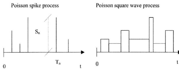
Considering the stochastic processes for the sustained live loads and the pulse type loads like wind, seismic and snow following assumptions are made: (1) sustained live load can be modeled as Poisson square wave process; (2) pulse type loads can be modeled as Poisson spike processes. The graphical presentation of Poisson square process and Poisson spike process is given in Figure 1:
Poisson spike process
... ... S l l
1 ... y::il ... 1 ...
i v / , /
Poisson square wave process
...
[
, ... liiiiiiiiiiiiiiiiiiiiii:i::iiii ... ]1 ... ... ...
I "
T,, 0 t
0 t
Figure I Graphical presentation of Poisson spike and Poisson square wave processes
The durations of Poisson spikes are assumed to be neglicible in comparison to the inter-arrival times of the pulse process. Further, the pulses are mutually independent and identically distributed with the cumulative distribution function Fi(x) and Poisson process intensity parameter ci for the i th spike process. Then the probability that a load pulse with amplitude larger than x occurs in the time interval from t to t + At in the i th process is equal to ci(1-Fi(x))At. Thus the counting process that counts the number of load pulses with amplitude larger than x is a Poisson process with intensity
ci(1-Fi(x)).
For the sum of the m compound Poisson spike processes we therefore have that the corresponding counting process is a Poisson process N(t) with intensity cl(1-Fi(x)), + ... + Cm(1-Fm(x)). The probability (i.e. the PDF of the extremes of the sum process) that there is no load pulse with amplitude that exceeds x within the interval [0, T] for the sum process of m Poisson spike processes is thusEquation 3 F s p i k e _ s u m ( X ) --
exp(-TEci(1-Fi(x))
In Equation 3 the summation index goes from 1 to m. This model is applicable if the load pulse durations are neglicible in relation to the inter-arrival times between the load pulses in all the load processes that are considered for combination. If this assumption is not valid Equation 3 can be corrected so that it takes the possibility of overlapping load pulses into consideration. The correction procedure is reasonable, only if the load pulse durations are essentially shorter than the time distances between the load pulses. If the overlapping of pulses is considered Equation 3 takes the following form for the sum of three spike processes
3 3 3
Equation 4 Fspike_sum(X ) -exp{-T[ Z
Ci(1-Fi(x))
+ E Z cij(1-Fi+j(x))f=l i j
3 3 3
+ EEE
Cijk(1-Fi+j+k(X))] }
i j k
In Equation 4 cij and Cijk in the double and triple sums are given by the following formulas
Equation 5 cij = cicj(E(Di) +E(Dj)); cicjck = cicjCk(E(Di) +E(Dj) + E(Dk))
In Equation 5
Di,
Dj, Dk are expected values of pulse durations in i, j and k processes, respectively.Fi+j
andFi+j+k are
the extreme value cumulative probability distribution function of sums of the pulse amplitude distributions for processes i, j and i,j,k, respectively. Indices i,j and k in sums of Equation 4 do not take identical values. In general case of n processes Equation 3 takes the formEquation 6
m
F s p i k e _ s u m ( X ) -
exp(-T E(n- 1)!EE... ~
n=l il i2 in
An exact solution exists for the sum of a compound Poisson spike process (process 1) and a Poisson square wave process (process 2) [7]. Following the notation of reference [6] we can write
Equation 7 Fspike+square(X)=g(T,x)exp(-c2T)
In Equation 7 the function g(T,x) satisfies the Volterra integral equation of the following form Equation 8 F(t,x) +c2 F(t-u,x)g(u,x)du- g(t,x)
where
Equation 9 F(t,x) - fx2(x-y)exp{-clt[1-Fxl(y)] }dy
A P P L I C A T I O N 1
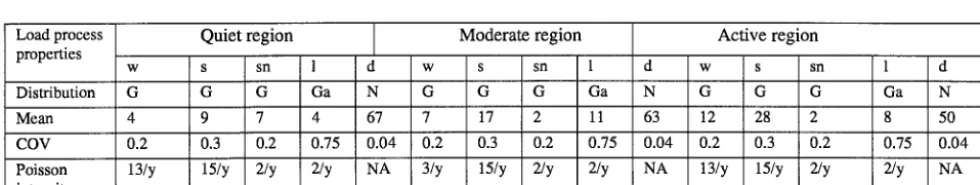
The application example tbe analyzed in this subsection considers as a sample structure the outer containment shell structure in the nuclear power plant. Typically, this building is reinforced concrete cylinder with flat top dome. The wall thickness in the shell is of the order of 50 centimeters. In order to normalize the load effect vertical stress component in the outer surface of the bottom of the shell in the leeward site for wind and seismic effects is investigated. The typical ratios of dead, live and environmental loads are taken approximately to correspond the quite, moderate and active regions in the world considering the seismicity and wind velocities during hurricanes. The snow load is taken for quite seismically quite area to correspond the snow loads in nordic countries. Using these assumptions and normalizing the sum of mean values of contributions of different loads to the investigated vertical stress to be 100 for every investigated region the summary table for stochastic properties of wind, seismic, snow, live load and dead load effects can be written as follows:
Load process properties Distribution Mean COV Poisson intensity
Quiet region
w s sn 1
G G G Ga
4 9 7 4
0.2 0.3 0.2 0.75 13/y 15/y 2/y 2/y
I
d N 67 0.04 NA
Moderate region
w s sn 1
G G G Ga
7 17 2 11
0.2 0.3 0.2 0.75 3/y 15/y 2/y 2/y
Active region
d w s sn 1 d
N G G G Ga N
63 12 28 2 8 50
0.04 0.2 0.3 0.2 0.75 0.04 NA 13/y 15/y 2/y 2/y NA
T a b l e 1 L o a d p r o p e r t i e s u s e d in the a p p l i c a t i o n e x a m p l e s o f the p a p e r . T h e f o l l o w i n g a b b r e v i a t i o n s are u s e d in the table: G = G u m b e l e x t r e m e v a l u e d i s t r i b u t i o n ; G a = G a m m a d i s t r i b u t i o n ; N = n o r m a l d i s t r i b u t i o n ;
w = w i n d ; s = s e i s m i c , sn = s n o w ; 1 = live load; d = d e a d load; y = y e a r
The load statistics for wind, live and dead loads given in table 1 were taken from reference [8] and for snow and seismic loads from references [9] and [ 10]. The life time of the structure was taken to be 50 years.
R E S U L T S O F A P P L I C A T I O N CASE 1
Combination of wind+seismic+snow+live+dead loads. Environmentally active region
1
0 9
0.8
o 7
. ~ 0 6
m
"~ 0 5
04
0 3 0.2 0 1 0
, 8 m
0 50 100 150
vertical stress
jm
v
~ d e a d _ w e i g h t
~ t o t a l c o m b i n a t i o n - 0,, w i n d
- 13= seismic
I I I s n o w
= :;~ live
! I
J
200 250
Figure 2 Load combination diagram for environmentally active region
Combination of wind+seismic+snow+live+dead loads. Environmentally moderate region
0.9
i
0 8 .
I
0 7 ,
~ 0 5 i " ~ _ ~ ~,
0 3 r ~ r ~ : '
0.2 ~I~.
o 50
I
J ~ d e a d _ w e i g h t
~ t o t a i combination
= <Y' w i n d
" ~ seismic
I ~ snow
I 0 0 150
verticalstress
200 250
Figure 3 Load combination diagram for environmentally moderate region
0.9 0 8 0 7
Z ' 0 , 6
e~ o
~. 0.4
0 3
0.2
0 1
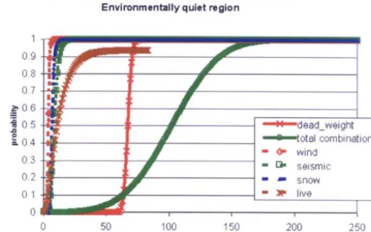
Combination of wind+seismic+snow+live+dead loads. Environmentally quiet region
I
0 50
i
~ d e a d _ w e i g h t
~ t o t a l corn bi nation
- O= w i n d
,= !:~ s e i s m i c
i m S l 7 0 W
" : ~ live
... i ... , . . . i ... t
100 150 200 2 5 0
vertical stress
DISCUSSION OF A P P L I C A T I O N CASE 1
The most important results are summarized for 95% fractiles in the following table 2:
Region Dead Live Wind Seismic Snow
Active 53.5 21 16.5 43.5 3
Moderate 68.5 28.5 16.5 26.5 3
Quiet 71.5 35 5.5 14.5 9.5
Combined 240 172 151
Table 2 Summary table of the load combination at 95% fractile location of distributions
If the obtained combined values for 95% fractile are compared to codified partial safety factor combination rules for characteristic load values that usually are the 95% fractiles from load distributions, we obtain with the partial safety factor of 1.5 for wind, seismic and snow, for partial safety factor 1.0 for dead and 1.3 for live [13] the value 175 for active region, the value 173 for moderate region and the value of 161 for quiet region. It can be seen that the actual load combination is quite sensitive to the ratios that individual load effects have to the total effect, whereas the codified combination does not seem to take this fact into account.
A P P L I C A T I O N CASE 2 V E N T I L A T I O N S T A C K F R A G I L I T Y OF LOVIISA NPP
The task in this assignment is to analyse the ventilation stack fragility of the Loviisa NPP. The stack is 107.5- meter high reinforced concrete cylinder and it serves both units of the Loviisa plant. The geometrical configuration of the stack is as follows. The outer diameter of the stack is constant for the whole length of the stack and its value is 6.8 meters. The uppermost segment of the stack is 62.5 meters high. Its wall thickness is 200 mm and its reinforcement percentage is 0.4. The middle portion of the stack is 22 meters high and its wall thickness is 400 mm and reinforcement percentage 0.4. The lowermost segment of the stack is 19 meters high to the top of the foundation and its wall thickness is 600 mm and its reinforcement percentage is 1.2. The side length of the rectangular foundation block is almost equal in both principal directions and the sidelength is about 12 meters. If the ribbed foundation is converted to solid rectangular block its heigth is about 2.5 meters and its total weight is 7.14 MN.
The foundation soil underneath the foundation is solid rock with only very moderate weathering. In this fragility analysis the rock stiffness characteristics are utilized for evaluating the spring constants for soil-structure interaction problem for evaluating the eigenfrequencies and natural mode shapes of the stack. The spring constants were developed using the elastic half-space theory. The obtained spring constants are frequency independent.
The load for which the stack fragility is evaluated is the mean hourly wind speed load. This load parameter has a wide statistical database of measured values from various regions of the world and is therefore suitable for characteristic parameter against which the stack conditional failure probability is evaluated in all investigated stack sections.
The sections chosen for fragility evaluation are the locations where the stack wall thickness varies discontinuosly, namely, +45.00 meters and +23.00 meters and the section at the top surface of the foundation at elevation +4.20 meters as well as the bottom surface of the foundation block at elevation-0.70 meters.
Characteristics of Wind Load
The effects of wind can be divided to static effects of basic mean wind speed and dynamic effects of temporarily varying wind speed like gust effect and vortex shedding and the structural response to these effects. For the definition of long time average "mean" wind speed different time span have been used like 10 minutes average speed~or hourly average speed. The gust effects are random in nature in both space and time. Davenport [14] has separated the gust effects as follows:
1. Wind "gust" loads which may be applied to only parts of the structure at any one time
2. Wind gusts at higher frequencies which are amplified by resonance at the natural frequencies of the structure
The structural responses for each this kind of wind load is potentially quite different and the modern research in wind engineering has been developing usable simplifications for different types of structures.
One of these simplifications is so called static gust approach, which is used for structures with negligible resonant response. It takes into account the long time average "mean" wind speed and the wind gusts applicable only to parts of the structure at any one time.
The gust load takes into account of wind fluctuations and depends on natural frequency, damping and height and width of chimney and is proportional to turbulence intensity. The basic mean wind speed to go along with turbulence intensity in the static gust models has been chosen to be either a "hourly" or "10 minute" mean wind speed.
Means are used because they are the most statistically stable measure of a randomly fluctuating value in any short-term record. The most modem wind codes such as Euro code 1 (EC1) [16] and UK standard BS 6399: Part 2 [17]
Wind standards use a variety of different methods to describe how the wind speed or wind pressure varies with height. The most common are exponential function type profiles, which are used for numerical simplicity. Logarithm function type profiles provide a better physical fit to the boundary layer effect in fluid flows. The basic explaining character in practical wind profile models is that the profile depends only on local surface roughness.
A model of a random process like wind must be based on statistically stable data. The local factors affecting the wind speed are:
1. 2. 3. 4. 5.
Local obstructions
The general roughness of the ground upwind
Changes of the ground roughness with distance upwind of the site Topography on site
Atmospheric stability on site
The storm mechanism by which strong winds are generated is also important. Most research has been of wind caused by large-scale extra-tropical cyclones. Other kind of wind gusts, for example gusts due to thunderstorms have different characteristics and different damage potential. Thunderstorm structure data have been classified from the nature of damage to trees. Site-specific information concerning thunderstorms is very difficult to obtain due to their infrequency at any particular site.
Normal extra-tropical cyclonic winds are easier to study because they occur all the time in temperate latitudes and are very common all around the world.
The ESDU (Harris and Deaves) Wind Model [18]
The work carried out by David Deaves and Ian Harris and Engineering Science Data Unit (ESDU) indicated the importance of two factors in developing the wind models. These factors are:
Displacement height, which is the direct and immediate effect of reasonable dense upwind obstruction, such as buildings or woods. This also causes the wind to be displaced upwards.
Distance (fetch) where the changes of ground roughness occur. This affects both mean speed and turbulence intensity
The ESDU methods give also a way of statistically relating gust and mean wind speeds at a particular location through an equation of the form
Equation 10 V l s - W (1
+glslu)
Where Iu is the turbulence intensity and for 1 second gust the expected value of the peak factor, gls, over one hour is 3.4.
Using peak factor 3.4 and the Equation 10, it is possible to derive gust speeds from information of mean speed and turbulence intensity.
The equation for gust factor derived from ESDU model is as follows:
Equation 11 G - 1 + 2 gls Iu +(gls Iu )2
The CICIND Model Code Model [15]
The CICIND model code assumes a single surface roughness and ignores the displacement height. These are i • very reasonable simplifications given the height and typical location of chimneys, Using the exponential function type profile, the mean wind velocity at different heights is determined from the basic wind speed. A mean wind pressure load is calculated using the mean speeds, while wind load due to gusts is calculated through the Equation 3 given below
Equation 12 G - 1 + 2gflu (B +ES/~)1/2
Notation in Equation 12 will be explained more in detail later when the CICIND model is applied to the Loviisa stack. Comparing ESDU and CICIND formulas (Equation 11 and Equation 12) it can be seen the term 2glu is common for both. The non-linear squared term at the end of Equation 11 is omitted in Equation 12 but Equation 12 has a square root term, which include the energy from low frequency gusts enveloping the chimney, B, and the resonant amplification of wind gusts at the natural frequencies of the chimney, ES/~.
Euro Code 1 Model [16]
Equation 13
Wgus t = Vmean (1
+7Iu)1/2
Stack Fragility Assessment
In order to assess the stack fragility the internal stress and resultant distribution because of mean hourly wind has to be determined. Statically the stack is relatively simple structure and the stress resultants can be determined with Excel-sheet for different basic mean hourly wind speed For evaluating the fragility in different sections of the stack the section stress resultants were also evaluated for several mean hourly wind speeds. For the sake of brevity these calculations are not presented in this paper. To assess the random variability of the section stress resultants as well as the uncertainty in the modeling of the structure for the determination of section forces, the internal force distribution was also determined with two different finite element models, namely, shell model and stick model. The same FEM-models were used as previously for calculating the stack natural frequencies and natural modal shapes.
The entire fragility family for an element corresponding to a particular failure mode can be expressed in terms
of the best estimate of the median load parameter capacity, Am and two random variables.
Thus, the ground acceleration capacity, A, is given by
Equation 14 A - Am ER EU
In which ER and Eu are random variables with unit medians, representing, respectively, the inherent randomness about the median and the uncertainty in the median value. In this model, we assume that both ER and eu are log-normally distributed with logarithmic standard deviations, [3R and [3u, respectively. The formulation for fragility and the assumption of lognormal distribution allows easy development of the family of fragility curves, which appropriately represent fragility uncertainty. For the quantification of fault trees in the plant system and accident sequence analyses, the uncertainty in fragility needs to be expressed in a range of conditional failure probabilities for a given load parameter value. This is achieved as explained below:
With perfect knowledge (i.e., only accounting for the random variability, ER), the conditional probability of failure, fo, for a given load parameter level, a, is given by
Equation 15 f0 = (I)[ln(a/Am)/~R]
where ((I)(.) is the standard Gaussian cumulative distribution function. The relationship between f0 and a is the median fragility curve.
When the modeling uncertainty eu is included, the fragility becomes a random variable (uncertain). At each load parameter value, the fragility f can be represented by a subjective probability density function. The subjective probability, Q (also known as "confidence") not exceeding a fragility f' is related to f' by
Equation 16 f' = (I)[ {In(a/Am) + ~u(I ) -I(Q) }/[3u]
Q = P[f<f'/a] i. e., the subjective probability (confidence) that the conditional probability of failure, f, is less than f for a peak load parameter value a;
O-I0 = the inverse of the standard Gaussian cumulative distribution function.
The median load parameter capacity Am , and its variability estimates [3R and [~u are evaluated by taking into
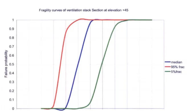
account safety margins inherent in capacity predictions in structural analysis and uncertainty structural modelling. For Loviisa ventilation stack the result of the fragility analysis against the mean hourly wind effects can be
summarized using the fragility model parameters Am - 2 5 m / s , [~R -" 0.1 and [3u - 0.2 and in the following Figure:
Fragility curves of ventilation stack Section at elevation +45
0.9
0.8
O.7
~
0.6o ~ - " ' m e d i a n
~. 0.5 i i i i ' - " ' - 9 5 % frac
G)
i - - ' 5 % f r a c
~
0.40.3
i
0.2
0.1
~
o !
0 5 10 15 20 25 30 35 40 45 50 55 60
Basic wind speed (hourly mean at 10 m height) (m/s)
CONCLUSION
For the investigated application cases the following concluding remarks can made. In the case of investigating the relative effect of different extreme environmental loads in areas of world with varying activity rates the ratios of component load effects to the total load effect seem to be a factor that has a significative influence on partial safety factors of loads in load and resistance factor design. This fact is not yet taken into account in codified safety factors for loads.
In the case of Loviisa ventilation stack fragility study the wind load was deemed to be deciding from the beginning of investigation and other load effects in the load combination were marginal. The Loviisa plant ventilation stack has its weakest section at elevation +45 meters. At this section the median value of the mean hourly wind capacity of the stack is 25 m/s. At this elevation all failure directions are as likely for the stack failure. Other investigated failure modes had higher capacities than bending failure at section at elevation +45. The expected gust wind speeds at Loviisa can be about 2.1 times as high as the hourly mean wind speed according to the CICIND - wind model used in the study.
REFERENCES
. 3. 4. 5.
° 10.
11. 12. 13.
14.
15.
16. 17. 18.
"Basic notes on actions." (1976). Appendix to the Bulletin CEB, No. 112, Comite Europeen du Beton, Paris, France.
E. Parzen (1962) Stochastic Processes. Holden-Day, San Francisco.
Ferry-Borges, L, and Castanheta, M. (1971). Structural safety. LNEC, Lisbon, Portugal.
A. M. Hasofer (1974) Time dependent maximum of floor live loads, J. Eng. Mech., ASCE, 100,1086-91. Y.-K. Wen (1990) Structural Load Modeling and Combination for Performance and Safety Evaluation. Developments in Civil Engineering, Elsevier, Amsterdam.
O. Ditlevsen, H. O. Madsen, (1996) Structural Reliability Methods, John Wiley&Sons, New York. A. M. Hasofer (1974) Time dependent maximum of floor live loads, J. Eng. Mech., ASCE, 100,1086-91. C. Floris (1998) Stochastic analysis of load combination, Journal of Engineering Mechanics, ASCE, September 1998.
Code for structural loads, Finnish Association of Civil Engineers, RIL 144-1990.
P. Varpasuo, (1999) Estimation of Seismic Hazard in Territory of Southern Finland, Proceedings of
OECD/NEA Workshop on Seismic Risk, August 10-12,
1999,
Tokyo, Japan.MATHCAD, (1995) User's Guide, Ver. 6.0, Mathsoft Inc., Cambridge, Massachusetts.
MATLAB, Optimization Toolbox, User's Guide, Version 2, Mathworks Inc., Natick, Massachusetts, 1999. ASME (1995), Boiler&Pressure Vessel Code, Division 2, Code for concrete reactor vessels and containments, ACI Standard 359-95, American Society of Mechanical Engineers
Davenport A.G., Isymov N. , Miyata T. : " The experimental determination of the response of suspension bridge to turbulent wind", Proc. Of the 3 rd Intern. Conf. On Wind Effects on Buildings and Structures, Tokyo
1971, p 1207-1209, Tokyo, Saikon Co. Ltd.
CICIND, 1998, Model code for concrete chimneys, Part A: The chimney shell. International Committee for Industrial Chimneys (CICIND) Switzerland.
Eurocode 1," Design loads for buildings and structures"
British Standard BS 6399 "Design loads for buildings and structures" Part 2: Wind effects. Allsop A., "Blowing in the wind : A critique of the EC1 wind speed proposals",