A Rapid Assessment Tool for Determining Uniformity if Irrigation Type Manure Application Systems

(1)

ABSTRACT

LIU, ZHENGZHONG. A Rapid Assessment Tool for Determining Uniformity of Irrigation-Type Manure Application Systems. (Under the direction of Garry Grabow.)

Due to the extent of the animal industry in North Carolina, the treatment of liquid manure is

of great importance. Since liquid manure contains plant nutrients, it is usually treated through

application to agricultural land through irrigation systems as a substitute or partial substitute

for commercial fertilizer. However, land application of liquid manure needs to follow some

guidelines in order to achieve economic goals as well as to protect the environment. Current

guidance suggests calibration of land application equipment be performed once every three

years by the “catch can” method, a time- and labor-consuming method. The research goals of

this project were to investigate the relationship between liquid manure application uniformity

and application system hydraulic measurements and then make tables of the predicted

application uniformity for field use.

Trials were performed to test the manure application uniformity for different sprinkler types,

nozzle types, gun models, nozzle diameters, system types, site types, gun models, and nozzle

pressures. The wind speed and direction during the trials was monitored. Different overlaps

were achieved by superposition, thereby allowing for assessment of multiple sprinkler

overlap extents for one trial. The overlaps used for traveling gun systems reflected sprinkler

(lane) spacings of 70%, 75%, 80%, 85%, and 90% of the wetted diameter, and those used for

stationary systems reflected sprinkler (lane) spacings of 50%, 55%, 60%, 65%, and 70% of

the wetted diameter. Including pseudo-observations, there were 722 records. Regression

models were constructed using trial data through processes of main effect selection,

collinearity checking, interaction term and quadratic term selection, parameter estimation,

and residual normality testing. The variables “sprinkler spacing in percent of wetted

diameter” and “wind speed” exist as quadratic terms in most of the models. Tables were

made using predictions from the selected models. The model for stationary systems performs

(2)

tendencies of application uniformity to predictive factors. The model for traveling gun

systems does not perform as well as that for stationary systems. The adjusted R2 is only 0.14, though low value is not unexpected due to the variance and conditions of the systems

(3)

A Rapid Assessment Tool for Determining Uniformity of Irrigation-Type

Manure Application Systems

by

Zhengzhong Liu

A thesis submitted to the Graduate Faculty of

North Carolina State University

In partial fulfillment of the

requirements for the Degree of

Master of Science

Biological and Agricultural Engineering

Raleigh, North Carolina

2009

APPROVED BY:

___________________________ __________________________

Rodney Huffman Jason Osborne

___________________________

Garry Grabow

(4)

ii

BIOGRAPHY

Zhengzhong Liu was born in Tongren, Guizhou Province, a small southwestern town of

China. Her father is a high school math teacher and her mother is a doctor practicing in a

hospital. She was curious about and wanted to go to America since she was in high school.

Afterwards, she applied for an undergraduate program of the Department of Computer

Science in Tongji University, Shanghai, China, because all the students in that Department

would be offered intern opportunities in the United States during their senior year. Despite a

high College Entrance Test score, she was not admitted to this Department. However, the

Department of Environmental Science and Engineering in Tongji University accepted her.

From then on, she began her studies related to water and wastewater, and she began to like

this field. In 2007, with her American dream and study interest, she became a Master‟s

student in the Department of Civil and Environmental Engineering in NC State University

and then transferred to the Department of Biological and Agricultural at the beginning of her

second semester. There, she took a research opportunity about field application of liquid

manure through irrigation systems. Having studied and lived in the United States for nearly

two years, she has learned a lot, not only in the academic realm but of American culture and

(5)

iii

ACKNOWLEDGEMENTS

I would like to acknowledge many people for their contribution to this research project. First,

I would like to thank my advisor Dr. Garry Grabow. Thanks for his guidance of the research,

thanks for his teaching, thanks for his help with my English speaking and writing, and thanks

for his courage. Without his care and help, I could not get used to t he new life and study

environment so quickly; without his academic guidance, I would not be able to achieve the

Master degree requirements; and without his contribution, this research project would never

become reality. I would like to thank Dr. Rodney Huffman. He impressed me with his

wisdom and “art”. Thanks for his careful guidance of the courses and presentations. Thanks

for his contribution to this research project. I would like to tha nk Dr. Jason Osborne and Dr.

Howard Bondell. Thanks for their professional guidance to help me analyze data and thanks

for their care to this research project. I would like to thank Dr. Willits to provide such great

seminar courses that help me a lot in my English speaking and writing.

I would also like to thank Carl Tutor and Trisha Moore. Carl helped a lot for the field trials

and Trisha helped me with my writing even during the busy final tests period. I would like to

thank my parents. They gave me support and courage. I would like to thank all the BAEers

(6)

iv

LIST OF FIGURES

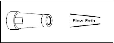
Figure 1-1 Taper Bore nozzle of model 100 gun ...11

Figure 1-2 Taper Bore nozzle of model 150 gun ...11

Figure 1-3 Construction of model 100 gun with Taper Ring nozzle ...12

Figure 1-4 Construction of model 100 gun with Ring nozzle ...12

Figure 1-5 Water distribution of a single sprinkler ... 124

Figure 1-6 Water distributions of sprinklers with overlap ...15

Figure 1-7 Water distribution of sprinklers with different overlaps ...12

Figure 1-8 Layout of the field determination of application uniformity for traveling gun system. The open circles represent catch cans and the “×” represents sprinklers. Adapted from AG-553-2 (Evans et al., 1997b). ...24

Figure 1-9 Layout of field calibration for stationary system. ...24

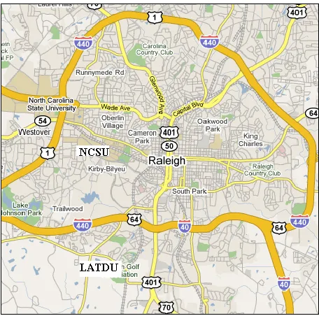
Figure 2-1 Locations of LATDU and NCSU...30

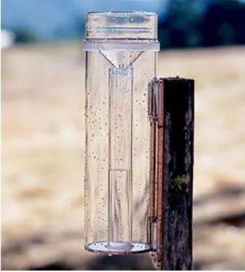
Figure 2-2 Rain gauge...32

Figure 2-3 Watchdog weather station ...33

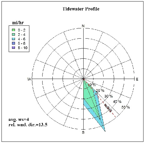
Figure 2-4 Example of wind rose diagram during a traveling gun system calibration ...33

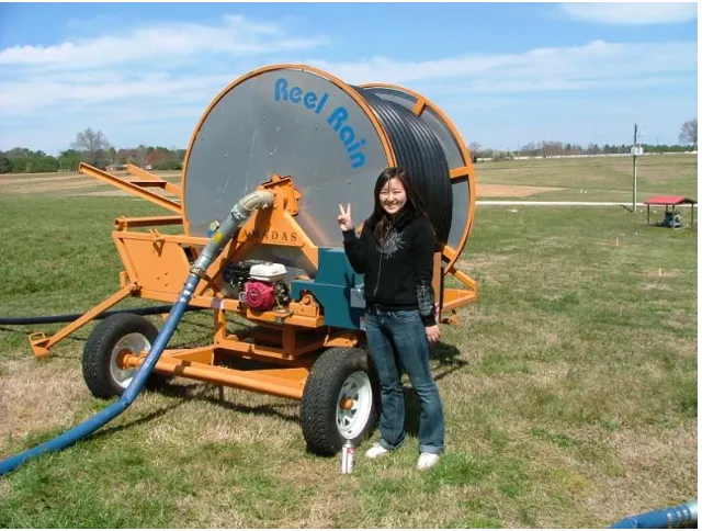
Figure 2-5 Reel Rain Traveler at LATDU...35

Figure 2-6 Nelson model 100 big gun. A-Taper Bore nozzle, B-Taper Ring nozzle, C-Ring nozzle ..35

Figure 2-7 Nelson model 150 big gun. A-Taper Bore nozzle, B-Taper Ring nozzle, C-Ring nozzle. 36 Figure 2-8 Nelson model 200 big gun. A-Taper Bore nozzle, B-Taper Ring nozzle, C-Ring nozzle. 36 Figure 2-9 Senninger 7025 impact sprinkler ...38

(12)

x

(13)

xi

LIST OF TABLES

Table 2-1 Data composition... 31

Table 2-2 Sprinklers, nozzle diameters, and nozzle pressures tested in traveling gun systems in both historic and study period... 39

Table 2-3 Sprinklers, nozzle diameters, and nozzle pressures tested in both historic and study periods ... 40

Table 3-1 Data composition... 54

Table 3-2 Selected variables form different selection methods ... 58

Table 3-3 Criteria of different models ... 59

Table 3-11 Criteria of different models... 78

(14)

1

1. Introduction

1.1. Background

North Carolina is one of the top meat producing states in the U.S. and the animal industry

plays an important role in the state‟s economy. In 1992, more than 30% of the state‟s farm

income was contributed by the animal industry, and more than 23,000 North Carolinians

worked in related areas (NCCES, 2007). In December 2007, the number of swine on the

farms in North Carolina was 10,200,000, ranking second among the United States after Iowa

(NCAS, 2007). Appropriate treatment and utilization of liquid manure is necessary,

otherwise it may cause environmental pollution.

One of the methods to handle liquid manure is to apply it to agricultural land through

irrigation systems. Liquid Manure is a very valuable agricultural asset since it contains many

nutrients and can be used as substitute or partial substitute for commercial fertilizers. Besides

providing nutrients, land application of liquid manure can help improve soil tilth, increase

water holding capacity, lessen erosion, improve soil aeration, and benefit soil

micro-organisms (Loehr, 1968). In North Carolina, every swine producer must submit a waste

management plan in which proper land application is designed to ensure the crops receive

nutrients uniformly and the environment is protected.

Irrigation methods and systems are categorized into several different types, including surface

irrigation, drip/micro irrigation, and sprinkler irrigatio n. Surface irrigation refers to systems

in which water is distributed by gravity flow through facilities such as a furrow, borderstrip

or basin; drip/micro irrigation (also called trickle irrigation) refers to systems that apply

water to individual plant through emitters or applicators located close to the plants; sprinkler

irrigation refers to systems that apply water by using pressurized piping systems with nozzles

(15)

2

traveling systems, hand move systems, stationary systems, and center pivot systems. Center

pivot systems can be used for irrigating most field crops (Burt et al., 1999). Hard hose

traveling gun systems and stationary systems can be used for field application of liquid

manure.

Sprinklers can be used for applying liquid manure, especially swine manure for it contains

less than 0.5% solids and does not tend to clog the pipes and sprinkler nozzles. In stationary

systems, impact sprinklers and “gun-type” sprinklers with nozzle size ranging from 0.25 in.

(6.4 mm) to 1.00 in. (25.4 mm) are used. The sprinklers or guns are fixed and set as a grid

throughout the field. Stationary systems work well for small and irregular-shaped fields and

require less labor than traveling systems. However, they have higher initial costs and the

impact sprinklers have small nozzles which are prone to clogging. In traveling systems, gun

sprinklers are used. The systems are operated by pulling out gun carts attached to hoses along

a travel lane and retrieving them slowly as liquid manure is pumped through the guns. The

hose is collected on a reel that is moveable. Since the systems are movable, they are more

flexible than stationary systems, and since the gun sprinkler is positioned relatively high on

the cart, it can be used with crops with a high canopy such as corn. Traveling gun systems

have the highest pressure requirement of any system (Keller and Bliesner, 2000) since they

need an additional 20-40 psi (140-280 kPa) to overcome the pressure losses caused by hose

friction during the delivery of water. The nozzle pressures range from 40-110 psi (276-758

kPa). They require more labor compared with stationary systems, and some land is lost to

production due to the traveling lane geometry.

1.2. Importance of application uniformity

Irrigation uniformity is related to the economics of the farming system and environmental

impacts since sprinklers cannot apply exactly the same amount of water throughout the field,

resulting in under- and over- irrigation. Applying insufficient water results in high soil

(16)

3

applied water results in leaching of plant nutrients and increasing disease incidence, under

which conditions crop yields will decrease (Solomon, 1990).

Seginer (1977) and Stern and Bresler (1983) have proven that crop yields are related to

irrigation uniformity. If water is applied uniformly throughout the field, which means that

every part of the crops or soil receive the same amount of water, the crops can attain

maximum yields. If the irrigation uniformity is poor, the crops yields will decrease.

Solomon (1983) provided a quantitative equation to show how sugar cane yield is affected by

the water applied:

y w 0.05 2.47w 2.19w2 0.77w3 0.10w4 (1.1)

where, y(w) = relative yield. It is the ratio o f actual yield to maximum yield

w = relative seasonal irrigation application. It is the ratio of actual applied water to

the amount of water resulting in the maximum yield

It is hard to determine by only inspecting the equation that how the relative yield changes

with the change of applied water. Some specific values were calculated based on equation 1.1

by Solomon (1983) to clarify the direct relationship between the relative yields and the

relative applied water. If the relative applied water is 1.00, the relative yield reaches 1.00. If

the relative applied water is either less or more than 1.00, the relative yield decreases. The

further the relative applied water departs from 1.00, the lower the relative yield. Therefore, it

is clear that the crops can give maximum yield only when receiving the right amount of

water. Either too much or too little applied water can negatively affect the yield. Since water

is critical to the crop and the application uniformity reflects water distribution, the

application uniformity must impact the yield. Solomon (1983) also gave a function to show

(17)

4

y(w) f₁ y w₁ f₂ y w₂ ... f_i y w_i (1.2)

where, y(w) = relative yield. It is the ratio of actual yield to maximum yield

fi = the fraction of the land that receives relative applied water wi

Based on the equation (1.2), assuming the relative yield is positive proportion of relative

applied water, when all the parts of the field ( f₁=100%) receive the yield maximizing amount of water (w_i=100%), the total relative yield is 100%×100%=1, resulting in the greatest possible yield. If only 30% of the field receives the yield maximizing amount of

water, 40% of the field receives 0.7 times this amount, and 30% of the field receives 1.2

times this amount, the resulting relative yield is30% 1.0 40% 0.7 30% 1.2 0.94, which is less than that from the system with perfect uniformity. Systems with higher water

application uniformity have greater crop yields.

1.3. Uniformity coefficients

1.3.1. Christiansen Uniformity

Application uniformity is evaluated by uniformity measures, which includes Christiansen

Uniformity (CU), Distribution Uniformity (DU), Scheduling Coefficient (SC) and some other

statistical terms. The Christiansen Uniformity Coefficient was first introduced by

Christiansen (1942) and is a function of the mean deviation and overall mean depth collected

by gauges or any other measures. The CU is calculated as:

100 1

CU

(1.3)

(18)

5

= average absolute deviation depth

= average application depth

The average deviation depth and the average application depth are the basis to the calculation

of CU. These two terms are defined in equations 1.4-1.5.

n

i i

y n y

1

(1.4)

Where, y=average application depth

i=the gauge number

n=the number of the gauges

yi=the depth of water in gauge i

1 | |

1

y y n

n

i

i (1.5)

where, δ=average absolute deviation depth

i=the gauge number

n=the number of the gauges

y=average application depth

yi=the depth of water in gauge i

CU treats the over application and under application the same and reflects the overall average

uniformity. If an application system has a CU of 100, every part of the field receives exactly

the same amount of water. A system with CU of 100 is ideal but not achievable. The lower

(19)

6

absolute deviation of the water depths equals the overall average water depth, the calculated

CU is zero, and when the average absolute deviation of the water depths is greater than the

overall average water depth, the calculated CU is negative. The zero and negative CUs may

happen in extremely unevenly irrigated areas, but they are hard to interpret. This is

considered to be a disadvantage of using CU as a uniformity index.

1.3.2. Distribution Uniformity

While CU puts emphasis on the overall water distribution, DU (distribution uniformity) and

DU50 (distribution uniformity of lower half) focus on the under- irrigated area. The theory behind the two coefficients is to use the range of the under-irrigated area and the overall area

to reflect the level of uniformity. DU was proposed by Dabbous (1962). It expresses the

uniformity as the ratio of the average depth of the collected water of the lowest quarter over

the grand mean depth and reflects the relationship between the driest quarter area and the

whole field:

DU 100( LQ) (1.6)

where, LQ = average applied depth of the lowest quarter = grand mean applied depth

DU = distribution uniformity

If DU equals 100, the application uniformity is considered “perfect” with the driest quarter of

the field receiving on average the same amount of water as the overall average. For example,

there are 8 catch cans labeled 1, 2, 3, 4, 5, 6, 7, 8, and the corresponding water depth in each

catch can is 1, 4, 1, 4, 1, 4, 1, and 4. Therefore, the overall averaged applica tion depth is 2.5

(20)

7

which means the averaged application of the driest quarter of the field is 60% lower than the

overall mean application. If there is no water applied to the driest 25% of the field, the DU

would be zero.

Another similar uniformity coefficient is Distribution Uniformity of the Lower Half. It is the

ratio of the average applied depth of the lower half to the grand mean of applied depth. It

reflects the relationship between the drier half and the whole field and is calculated as:

_DU₅₀ 100( Lh)_(1.7)

where, Lh = average applied depth of the lower half = general average of applied depth

DU50 = distribution uniformity of lower half

Similar to DU, a higher value of DU50 means a better uniformity. A DU50 of 70 means that the averaged application of the lower half area is 30% lower than the overall mean

application.

1.3.3. Scheduling Coefficient

Another quantitative evaluation of application uniformity is scheduling coefficient (SC),

which was developed by CIT (Center for Irrigation Technology) in conjunction with industry

representatives. It uses the relationship of the average application rate and the lowest

application rate in the sprinkler layout to reflect the application uniformity. SC is unique

since the value has meaning in terms of the scheduling of irrigation run time (Mgebroff,

(21)

8

LPR PR

SC (1.8)

where, PR = the precipitation rate of entire irrigated area

LPR = is the lowest precipitation rate in the irrigated area

SC = scheduling coefficient

SC indicates how much additional water is needed to adequately irrigate the dry spot, but the

size of the area used as the lowest irrigated area is not fixed. It can be for example, a

contiguous area of 2%, 5%, or 10% of the total area of coverage with the selected contiguous

area affecting the SC value. Similar to DU, SC focuses on the drier part of the field, but SC

requires that the driest area be contiguous while DU does not have this requirement. A

perfectly irrigated system has a SC value equal to 1, and poorer uniformity causes a larger

value of SC. A SC value of 1.5 means that the system needs to run 1.5 times as long as the

run time calculated using the average application rate to apply the target amount of water to

the driest contiguous region of the irrigated area.

1.3.4. Other statistical measures

Some statistical measures are also used to evaluate the application unifo rmity, such as CV

(coefficient of variation) and CAV (coefficient of average variation). They measure the

variability of the depth of applied water (Mgebroff, 1991). Dukes (2006) used the CV of the

application depth in catch cans to reflect the application uniformity. The related equations

are:

CV SD

M (1.9)

where, CV = coefficient of variation

(22)

9

M = Mean of the distribution

AD CAV

M (1.10)

where, CAV = coefficient of average variation

AD = average deviation

M = Mean of the samples

1.3.5. The relationship between uniformity coefficients

All of the uniformity coefficients described previously are related. If one coefficient shows a

poor uniformity, the others show it too. Many previous studies found linear relationships

between CU and DU. Keller and Bliesner (2000) provided two commonly accepted t

relationships:

CU 100 0.63(100 DU) (1.11)

or

DU 100 1.59(100 CU) (1.12)

For normally distributed data, CU equals DU50 (Burt et al., 1999). Mgebroff (1991) stated that when the lowest contiguous 25% of the entire field is used as the lowest irrigated area,

the calculated SC becomes the inverse of DU. The relationship of DU and CV of normally

distributed data was presented by Hart (1961), as shown in equation 1.13.

(23)

10

The relationship between DU50 and DU is shown in equation 1.14 (IA, 2005):

DU_{5 0} 0.386 (0.614 DU) (1.14)

Although uniformity coefficients are related, they have different meanings and should be

chosen based on objectives such as yield and, in the case of liquid manure application,

potential environmental degradation. They can be used together to provide more information

to the operators of animal waste application systems.

1.3.6. The use and inte rpretation of Christiansen Uniformity

Application systems differ in their ability to achieve recommended or prescribed uniformity

levels. With various recommended acceptable CU values in the literature, there is not a

uniform rule to decide whether the CU is acceptable. Evans et al., (1997a), state that a CU

greater than 75 is considered to be excellent for a stationary system of liquid manure

application. A CU from 50 to 75 is considered to be good and is acceptable, while a CU less

than 50 is considered as poor uniformity and not acceptable. Traveling gun systems can

commonly achieve a CU greater than 85 if a proper overlap is set (Evans et al., 1997b). A

CU between 70 and 85 is considered to be good and is acceptable for traveling gun systems

of liquid manure application. A CU lower than 70 is unacceptable for traveling gun systems

of liquid manure application and the systems are required to be adjusted. Wright and Cross

(1996) pointed out that the acceptable CU for traveling gun systems is 85. Cuenca (1989)

recommended CU to be 80 for field crops and 85 for specialty crops based on the crop value

and equipment costs in a fresh water application system. Keller and Bliesner (2000) stated

that the CU value should be 75 or above for general field and forage crops and 84 or above

for high value crops. Mgebroff (1991) stated that acceptable values of CU are 80 and above

(24)

11

1.4. Factors affecting Application uniformity

There are many factors that may affect the water distribution of a sprinkler and application

uniformity of the system. Those are sprinkler model, nozzle type, nozzle size, nozzle

pressure, and sprinkler spacing, all of which are controllable in field trials. The most

important uncontrollable factor is wind (Solomon, 1979).

1.4.1. Nozzle type, gun model, and nozzle size

Sprinklers have different constructions and they may be categorized by 1) models (sizes); 2)

nozzle types; and 3) nozzle diameters. The Nelson big gun, for example, has four different

models (75, 100, 150, and 200) and three different nozzle types (Taper Bore, Tap er Ring, and

Ring). Each sprinkler with a specific nozzle type and gun model contains various nozzle

diameters. Normally, a model 200 gun uses a bigger nozzle diameter than a model 150 gun,

and a model 150 gun uses a larger nozzle diameter than model 100 gun. Figures1-1 and 1-2

show gun models 100 and 150 with a Taper Bore nozzle. Figures1-1, 1-3, and 1-4 (From

Nelson Irrigation Corporation website) show a model 100 gun with different nozzle types.

Figure 1-1 Taper Bore nozzle of model 100 gun

(25)

12

Figure 1-3 Construction of model 100 gun with Taper Ring nozzle

Figure 1-4 Construction of model 100 gun with Ring nozzle

Different physical characteristics of nozzle types, gun models, and nozzle diameters cause

different sprinkler performance as measured by water distribution patterns. Dukes (2006)

tested the application performance of IWOB (wobbling diffuser nozzles) sprinklers and LDN

(low drift nozzles) sprinklers. IWOBs use a diffuser to provide a random pattern of droplets,

and LDNs are developed to resist stream distribution under windy conditions. The results

showed that the IWOBs always give a higher uniformity than LDNs in terms of CU and DU.

Although IWOBs are not used for liquid manure application, it shows the effect of sprinkler

construction on the water distribution and application uniformity. Tarjuelo et al. (1999a)

found a 0.19-in. (4.8- mm)- nozzle Agro 35 sprinkler achieves better uniformity than a 0.19 in.

(4.8 mm)- nozzle Rain Bird 46 sprinkler at 44 psi (300-kPa) nozzle pressure and 59×59ft

(26)

13

1.4.2. Nozzle pressure

Nozzle pressure determines the velocity of the water flow and the size of the droplets coming

out from the nozzle. The droplet velocity affects the resistance of the air to the droplets, and

thus affects the airborne duration of the droplets and their fall velocity. The fall velocity of a

droplet is proportional to the square of its drop size. If the nozzle pressure is too high, there

are mainly fine droplets, which easily drift and can be blown far away from the sprinkler by

strong wind. If the nozzle pressure is too low, there are mainly large droplets. Those big size

droplets have high fall velocities and large resistance from the air that reduces the horizontal

speed. Therefore, they also land very close to the sprinkler, and the high fall velocity causes

soil dispersion (Rupar, 1978). Droplets landing too close to the sprinklers means that the

wetted diameter is reduced, thus the application uniformity is decreased if other factors are

fixed. Additionally, an extremely small pressure will cause improper jet break up. Only under

the proper nozzle pressure does the water from the sprinkler distr ibute effectively.

Sprinklers are designed to operate within a recommended pressure range that is provided by

the manufacturer or system designer. The effects of nozzle pressure on application

uniformity have been studied in many previous studies. Dukes (2006) conducted a series of

experiments with IWOB sprinklers and LDN sprinklers under different pressure ranges. Both

of the two kinds of sprinklers showed lower irrigation uniformity at system pressure range of

9-14 psi compared to 29-42 psi. When the wind speed was less than 1.7 m/s, the range of CU

of LDN sprinklers was as large as 12 for different system pressures. An additional benefit of

adequate operating pressure is that uniformity is less affected by nozzle wear or age (Louie

and Selker, 2000).

1.4.3. Sprinkler and Lane spacing

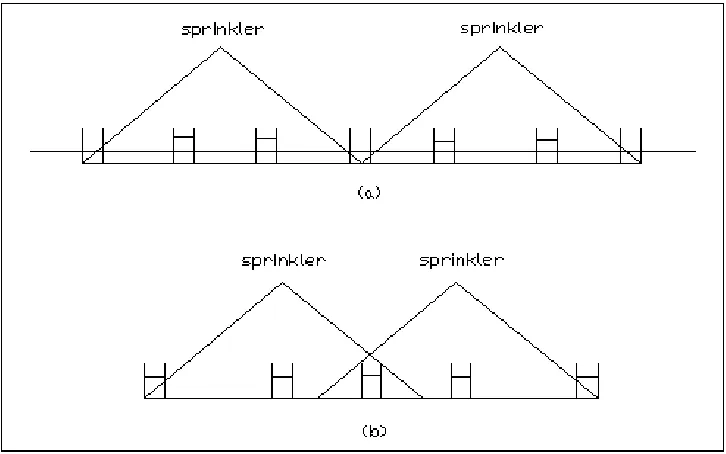
The water distribution of a single sprinkler is not uniform. A sprinkler applies much more

water to the area near it than the area far from it (figure 1-5). So, if only one sprinkler is

(27)

14

poor application uniformity can be alleviated by the introduction of “overlap”. As shown in

figure 1-5 and figure 1-6, the water deficit of the area receiving little water from the sprinkler

located in the middle area is made up by the water applied by other adjacent sprinklers, thus

greater application uniformity is produced. Overlap reflects how much the applied water is

superimposed and is normally represented by sprinkler spacing in percent of wetted diameter.

When determining the wetted diameter, three flags are used to mark three observations of the

furthest point wetted on either side of the gun. The distance between the averaged flag on

both sides is the wetted diameter of the sprinkler (Evans et al., 1999). Lane spacing is an

equivalent of sprinkler spacing for traveling gun systems.

(28)

15

Figure 1-6 Water d istributions of sprinklers with overlap

Overlap or sprinkler spacing affects the water amount received by each catch can, and thus

affects the application uniformity. Figures 1-7a and 1-7b show the application uniformity

under different sprinkler spacing. The rectangles represent the depths of collected water. In

figure 1-7a, the sprinklers are further apart (wider sprinkler spacing), thus giving larger

sprinkler spacing, compared to figure 1-7b. The water amount received by the catch cans in

figure 1-7a is less uniform than those in figure 1-7b, thus the system in figure 1-7b produces

better application uniformity. Generally smaller sprinkler spacing provides greater

(29)

16

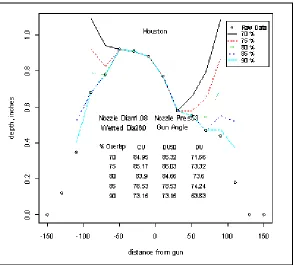
Figure 1-7 Water distribution of sprinklers with different overlaps

However, setting overlap or sprinkler spacing is a trade-off because closer spacing, while

increasing uniformity, increases initial cost. A sprinkler spacing of 70 to 80 percent of the

wetted diameter is recommended for traveling gun system (Evans et al., 1997b), while a

sprinkler spacing of 50 to 65 percent of the wetted diameter is recommended for stationary

systems (Evans, et al., 1997a).

1.4.4. Wind

Wind plays a great role in application uniformity. Rupar et al. (1978) stated that the

application uniformity is affected most by wind at any given sprinkler spacing in a traveling

gun system. The mechanisms by which wind affects the application uniformity are water loss

by drifting small droplets and distorted water distribution patterns (Seginer et al., 1991; Han

et al., 1994). Seginer et al. (1991) reported that the total drift can be formulated as a function

(30)

17

Wind affects the application uniformity in two ways: wind speed and direction. The wind

interacts with the water discharged by the sprinklers. When the nozzle is pointing upwind,

the resistance of the air to the stream is more than normal, and larger drops are broken down

into smaller drops, which are slowed by the wind more than big drops, thus producing a

distortion of the distribution pattern. When the nozzle is pointing downwind, the resistance of

the air to the stream is less than normal, and there are fewer small drops. In short, the wind

will shorten the upwind wetted radius and lengthen the downwind wetted radius. Han et al.

(1994) pointed out that wind speed moves a pattern‟s center of gravity to new location

leeward, stretches the pattern along the wind direction, and shrinks the pattern in the

perpendicular direction. This is the reason that most common models of water distribution

patterns affected by wind are elliptical.

Many studies have been designed to characterize the effect of wind on application

uniformity. Different relationships between application uniformity and wind speed have

been reported. von Bernuth and Seginer (1990) showed a linear relationship between the two;

Tarjuelo et al. (1992) showed a second-degree polynomial relationship between the two; and

later, after having conducted 94 tests, Tarjuelo et al. (1999b) found that a third-degree

polynomial equation provided the best fit for the regression of irrigation uniformity and wind

speed. Although different models have been developed to show the relationship of the

application uniformity and the wind speed, they all show that higher wind speed reduces the

irrigation uniformity. According to Standard S330.1 (ASABE, 1995), it is not recommended

to do field uniformity testing with wind speed greater than 5 mph (2.2 m/s) due to the

negative effect on application uniformity.

The effect of wind direction on irrigation uniformity is not as great as wind speed. Although

some studies show the existence of the effect of wind direction on application uniformity,

most studies conclude that there is little relationship between the two. Rupar (1978)

(31)

18

results showed a CU of 92 for all three conditions. Dukes (2006) found that the correlation

coefficient between CU and wind direction, in linear move irrigation systems, was as low as

-0.0019, which illustrated a negligible effect of wind direction on irrigation uniformity.

1.5. Field measures of application uniformity

1.5.1. The importance of field calibration

Land application systems should meet acceptable application uniformity to make sure that

they provide good agronomic performance and minimize environmental impact. However,

the application uniformity of the systems tends to decline with the age. There are various

reasons behind decline in uniformity, but usually it may be attributed to pump and sprinkler

wear. Struvite and other salts may also precipitate in the main lines, resulting in increased

head loss and lower sprinkler operating pressure.

In liquid manure land application systems, poor application uniformity has many

disadvantages. If liquid manure is over-applied to crops, the extra liquid manure will either

become runoff and pollute surface water or percolate below the crop root zone and pollute

the ground water. If liquid manure is under-applied to crops, larger manure storage facilities

and more commercial fertilizers are needed, which are added expenses. Therefore, the field

measurement and calibration of the application systems is necessary and should be performed

periodically.

The National Pollutant Discharge Elimination System (NPDES) permits issued by NC

DENR (North Carolina Department of Environment and Natural Resources) require that the

field calibration of animal waste application systems should be carried out once a year, and

the State General permits require calibration to be performed every other year. On September

1, 1996, the SB (Senate Bill) 1217 Interagency Committee, formed by the North Carolina

(32)

19

suggested that the calibration of liquid manure application systems should be done once

every three years by the “catch can” method (Evens et al., 1997, 2001). Later, in about 2005, Murphy Brown LLC proposed another method to “calibrate” liquid manure application

systems by comparing the flow rate measured by a flow meter against that in the

manufacturer‟s charts using measured nozzle pressure. In this procedure, if the difference of

the measured flow rate and that in the chart exceeds 10% or the difference of the measured

wetted diameter and that in the chart exceeds 15%, a technical specialist should be contacted

to diagnose the cause of poor performance. The “Murphy Brown” method is easier and

requires less time than the “catch can” method, but it sets an allowable difference between

the different ways of obtaining flow rates and wetted diameter, rather than comparing

measured values to design or permitted values. Additionally, there is no provision for

evaluation of uniformity. Recently, the eighth version of the SB 1217 guidance document

clarified that the measurement of the flow rate and wetted diameter of liquid manure systems

should be done every year, and the “catch can” method should be used at least once every

three years.

The parameters that need to be verified include flow rate (the rate water is applied to a given

area in terms of volume per time), nozzle pressure, wetted diameter (the farthest distance of

that a sprinkler can apply water to), and application uniformity. The results of the field

calibration procedures are used to determine whether there are problems and whether the

system needs to be adjusted by comparing with the parameter values provided by the system

designers or found in the wettable acreage determination for the site. This achieves the

overall goals of agronomic efficiency and environmental protection.

1.5.2. Determination of flow rate

Flow rate is a very critical parameter for it reflects not only the performance of the irrigation

system, but also the system‟s application rate. Flow measurement can be determined in two

(33)

20

manufacturer‟s chart. The accuracy of the pressure gauge should be within ±2% and of the

flow meter should be within ±3% in order to obtain acceptable measurements (ASABE

S330.1, 1995). When using a flow meter, flow rate may be determined either by observing

the instantaneous rate or from totalized flow over a known period. If the instantaneous flow

rate varies by 10%, the flow rate should be determined by recording the flow accumulated

over at least 15 minutes after the system is running steadily and dividing the accumulated

flow by the time. According to the SB 1217 document (2007), the acceptable difference of

the measured flow rate and the value specified in the irrigation design documentation or in

the wettable acreage determination is 10%.

Application rate is the rate that water is applied to a given area. It is usually expressed in

units of depth per time (Hoffman et al., 2007). Application rate partly determines the amount

of water and nutrient applied to the field. A high application rate exceeding the intake

capacity of the soil may result in loss of resources and pollution of surface water or

groundwater when deep percolation occurs. Improper application rates will reduce crop

yields. Application rate is chosen based on the crop type, soil type, and application time. The

relationship between flow rate and application rate is shown for stationary systems (Keller

and Bliesner, 2000):

e

K Q I

S S_l (1.16)

where, I = average application rate, mm/h, (in. /hr)

K = conversion constant, 60 for metric units (96.3 for English units)

Q = sprinkler flow rate, L/min (gpm)

(34)

21

and for traveling gun systems (Keller and Bliesner, 2000):

q

K Q I

V W t (1.17)

where, I = average application rate, mm/h, (in. /hr)

K = conversion constant, 60 for metric units (1.604 for English units)

Q = sprinkler flow rate, L/min (gpm)

W = tow path sprinkler spacing, m (ft)

Vq = travel speed, m/min (ft/min) t = application time, hr

1.5.3. Verification of Nozzle pressure and Wetted diameter

Sprinkler pressure affects the irrigation uniformity greatly because it affects the wetted

diameter. The manufacturer and the irrigation system designers provide a recommended

nozzle pressure range to make sure that the irrigation system operates as intended and

achieves acceptable uniformity. The nozzle pressure should be determined by a properly

functioning pressure gauge (SB 1217 Interagency Committee, 2007). A pitot tube attached to

the pressure gauge may be fixed against the jet issuing from the sprinkler nozzle when the

system is operated, and the nozzle pressure can be directly read from the pressure gauge.

Some sprinklers or sprinkler risers have ports for permanently installing pressure gauges and

the estimated nozzle pressure can be read from the mounted gauges. However it is not the

real nozzle pressure because it is not measured near the nozzle. Some charts differentiate between “base” pressure (base of sprinkler or on the riser) and nozzle pressure. The

measured nozzle pressure should be within the range recommended by the manufacturers or

(35)

22

The verification of wetted diameter is recommended to be performed by direct footprint

measurement (Evans et al., 1999). Footprint measurement involves observing the boundary

between wetted area and unwetted areas, marking the boundaries, and measuring the

distance. The measured wetted diameter is then compared with that in the manufacturers‟

chart with a specific nozzle pressure. A difference within 15% of the wetted diameter value

provided by the manufacturer is acceptable (SB 1217 Interagency Committee, 2007).

1.5.4. Determination of application uniformity

The “catch can” method is used in the field determination of application uniformity. The

theory behind it is to measure the collected depths of liquid manure in a sampled region of

the field to represent the water distribution throughout the whole field. The general procedure

includes setting out catch cans, operating the system, measuring the amount of liquid manure

collected in each can, and computing the application uniformity coefficient. The uniformity

coefficient is then checked against the performance categories as given in AG-553-2 (Evans

et al., 1997b). If a minimum standard is not met, owners of the system should contact an

irrigation dealer or technical service provider to determine the causes of poor uniformity.

Accurate measurement of water applied by sprinklers is necessary when determining the

amount of applied water (Kohl, 1972). The accuracy of measurement is affected by the type

and the number of the catch cans and the weather conditions. According to AG-553-1 (Evans

et al., 1997a), the containers should be the same size and be set at the same height relative to

the sprinkler. It is also suggested that the calibration should be performed over a low

evaporation period, which occurs with cool temperatur es and low wind speeds, to minimize

the error of catch depths caused by evaporation. According to ASAE Standard 330.1 (1995),

all the containers should be designed to minimize the splash of the liquid manure.

The arrangements of the catch cans in the field trials for determining the application

(36)

23

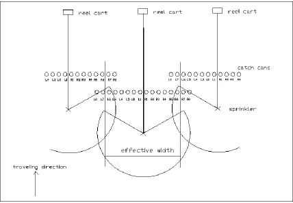
systems, the determination is implemented through placing a row of at least 16 catch cans

(Evans, et al., 1997b) as liquid manure collection containers, and linearly moving a gun

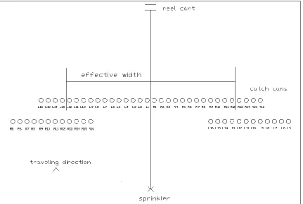
sprinkler perpendicular to and through the middle of the gauges (figure 1-8). In figure1-8,

the catch cans are labeled L1 to L8 and R1 to R8 where “L” means the left side of the

sprinkler and “R” means the right side of the sprinkler when facing the reel cart. The water

depths in the catch cans are immediately recorded after the system contributes no more liquid

manure to the cans.

The effective width of a sprinkler is identified by the accumulative distance from the

sprinkler to the point half way to the closest two sprinklers (figure 1-8) and is equivalent in

distance to the lane spacing. The effective width region is the area under which uniformity

calculations proceed. The outer cans would receive liquid manure from adjacent sprinklers,

so the liquid manure depths collected by these catch cans must be superimposed (left to right

and vice versa) and thus added to corresponding catch cans within the effective width. The

adjusted depths (after superimposing) are used to calculate the average application depth,

deviation depth, average deviation depth, and uniformity coefficient s through equations 1.3

(37)

24

Figure 1-8 Layout of the field determination of application uniformity for traveling gun system. The open circ les represent catch cans and the “×” represents sprinkle rs. Adapted from A G-553-2 (Evans et al., 1997b).

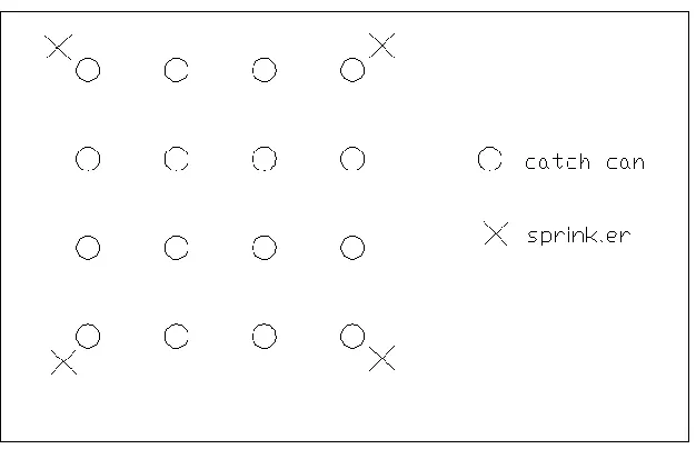
In the field determination of application uniformity of stationary systems (figure 1-9), four

adjacent sprinklers are selected and at least 16 catch cans are labeled and set in a grid within

the square area formed by the four sprinklers. The four sprinklers are operated for a full cycle

of operation time, and the liquid manure depths in these catch cans are recorded immediately

after the operation. Afterwards, the CU is computed from the average application depth,

deviation depth, average deviation depth, and uniformity coefficients based on equation 1.3

to equation 1.8. The liquid manure depths in this case do not require any superpositioning,

since those water depths have already taken account of the overlaps. There are several other

(38)

25

Figure 1-9 Layout of fie ld calibration fo r stationary system

1.6. Uniformity predicting software

There are various kinds of software for predicting application uniformity, such as “Overlap”

(Nelson Irrigation Corporation, Walla Walla, WA) which is used to predict the precipitation

rate and uniformity coefficients for specific sprinkler models and sprinkler spacings in

stationary systems; and “Winsipp” (Senninger Irrigation, Inc., Clermont, FL), which provides

the profile of water distribution, the uniformity coefficients, and application rates of specific

sprinkler models and pressures for Senninger sprinkler systems. These types of software

packages are very convenient in predicting irrigation uniformity in the design process.

However, they are not intended for field evaluation of application uniformity. Therefore, a

tool which is easy to use for the producers and has acceptable accuracy for an actual land

application is needed.

1.7. Study objectives

In this study, a series of field trials were conducted varying several factors including gun

model, nozzle type, nozzle size, nozzle pressure, sprinkler spacing, and wind. The main

(39)

26

Investigate the relationship between application uniformity and hydraulic

measurements.

Develop a series of tables for operators of animal waste systems to check liquid

manure application uniformity based on easily measured hydraulic variables.

Those series of tables are treated as “a rapid uniformity assessment tool”. The tables give the

relationship between the pertinent factors determined in the statistical model selection

processes and the uniformity coefficient (CU). If this uniformity tool can accurately predict

uniformity for liquid manure application systems, it may persuade the SB 1217 committee to

change their guidance in favor of this easier method. By predicting uniformity, this proposed

method would also help determine if a system is operated correctly or is in need of

maintenance or operational changes.

1.8. References

ASAE Standards, S330.1 SEP91. 1995. Procedure for Sprinkler Distribution Testing for Research Purposes. ASAE.

Burt, C.M., A.J. Clemmens, R. Bliesner, J.L. Merriam, and L. Hardy. 1999. Selection of Irrigation Methods for Agriculture. Reston, VA.: ASCE.

Christiansen, J. E. 1942. Irrigation by Sprinkling. California Agricultural Experiment Station Bulletin 670, University of California, Berkeley, CA.

Cuenca, R. H. 1989. Sprinkler System Design. Irrigation System Design. An Engineering Approach: 256-265.

Dabbous B. J. 1962. A study of sprinkler uniformity evaluation methods. MS Thesis. Logan, UT: Utah State University, Department of Agricultural and Irrigation Engineering .

DACS-NCAS. 2006. Agricultural Statistics of North Carolina. Raleigh, NC.: DACS North Carolina Agricultural Statistics.

(40)

27

Evans, R.O., J.C. Barker, J.T. Smith, and R.E. Sheffield. 1997a. AG-553-1, Field Calibration Procedures for Animal Wastewater Application Equipment - Stationary Sprinkler Irrigation System. NC Cooperative Extension Service & NC State University.

Evans, R.O., J.C. Barker, J.T. Smith, and R.E. Sheffield. 1997b. AG-553-2, Field Calibration Procedures for Animal Wastewater Application Equipment - Hard Hose and Cable Tow Traveler Irrigation System. NC Cooperative Extension Service & NC State University.

Evans, R.O., R. E. Sneed, R.E. Sheffield, and J.T Smith. 1999. AG-553-7, Irrigated Acreage Determination Procedures for Wastewater Application Equipment - Hard Hose Traveler Irrigation System. NC Cooperative Extension Service & NC State University.

Han, S., R.G. Evans, and M.W. Kroeger. 1994. Sprinkler Distribution Patterns in Windy Conditions. American Society of Agricultural and Biological Engineers 37(5): 1481-1489.

Hart, W.E. 1961. Overhead Irrigation Pattern Parameters. Agric. Engr. July. 354-355.

Hoffman, G. J., R.G. Evans., M.E. Jensen, D.L. Martin, R.L. Elliott. 2007. Design and Operation of Farm Irrigation Systems. 2nd ed. American Society of Agricultural & Biological.

IA. 2005. Landscape Irrigation Scheduling and Water Management. March 2005. Irrigation Association Water Management Committee. Falls Church, VA. 190 pp.

Keller, J. and R.D., Bliesner. 2000. Sprinkler and Trickle Irrigation. Caldwell, N.J.: Blackburn Press.

Kohl, R. A. 1972. Sprinkler Precipitation Gage Errors. Transactions of the American Society of Agricultural Engineers 15(2): 265-265, 271.

Loehr, R.C. 1968. Pollution Implication of Animal Wastes-a Forward Oriented Review. Ada, OK: Federal Water Control Administration, U.S. Department of the Interior. Robert S. Kerr Water Research Center

Louie, M. J. and J.S. Selker. 2000. Sprinkler Head Maintenance Effects on Water

(41)

28

Mgebroff, J. T. 1991. Uniformity Statistics for Describing and Comparing Water Distribution Data. IA Technical Conference: 126-138.

NCCES. 2007. The North Carolina Poultry Industry: May 2007. Raleigh, NC.: College of Agriculture and Life Sciences NCSU. Available at: http://www.ces.ncsu.edu/depts/ poulsci/tech manuals/poultryindustry.html. Accessed 29 July 2009.

Rupar, B. 1978. Optimizing Traveling Sprinkler System Performance. IA Technical Conference: 152-159.

Seginer I. 1977. A Note on the Economic Significance of Uniform Water Application. Irrig Sci 1: 19-25.

Seginer, I., D. Kants, and D. Nir. 1991. The Distortion by Wind of the Distribution Patterns of Single Sprinklers. Agricultural and Water Management 19: 341-359.

Solomon, K.H. 1979. Variability of Sprinkler Coefficient of Uniformity Test Results. Transactions of the American Society of Agricultural Engineers 22(5): 1078-1080, 1086.

Solomon, K. H. 1983. Coefficient of Uniformity. IA Technical Conference: 194-199.

Solomon K.H. 1990. Irrigation Notes-Sprinkler Irrigation Uniformity: August 1990. Fresno, CA.: CIT California State University. Available at:

http://cati.csufresno.edu/CIT/rese/90/900803/index.html. Accessed 29 July 2009.

Stern J and E. Bresler. 1983, Non-uniform sprinkler irrigation and crop yield. Irrig Sci 4: 17-29.

Tarjuelo, J. M., M. Valiente, and J. Lozoya. 1992. Working Conditions of a Sprinkler to Optimize the Application of water. Irri. Drain. Engng. 118(6): 895-913.

Tarjuelo, J. M., J. Montero, M. Valiente, F.T. Honrubia, and J. Ortiz. 1999a. Irrigation uniformity with medium size sprinklers Part I: Characterization of water distribution in no-wind conditions. Transactions of the American Society of Agricultural

Engineers 42(3): 665-675.

(42)

29

on Water Distribution. American Society of Agricultural and Biological Engineers 42(3): 677-689.

The North Carolina 1217 Interagency Group. 2007. Senate Bill 1217 Document. Raleigh, NC.

von Bernuth, R. D. and I. Seginer. 1990. Wind Considerations in Sprinkler System Design. Third National Irrigation System. St. Joseph, Mich.: ASAE.

(43)

30

2. Materials and Methods

2.1. Site description

The field trials were performed at LATDU (Land Application Training and Demonstrating

Unit) and on producer farms. The trials at LATDU are referred to as “controlled trials”,

because the test factors, such as system type, gun model, nozzle type, nozzle dia meter, and

nozzle pressure, could be set at pre-determined levels. The trials on producer farms were

referred to as “producer trials”, because the test factors were fixed at one operational level.

LATDU is a 24-acre site located at the Lake Wheeler University Field labs, 15 miles from

the campus of NC State University (figure 2-1). Since liquid manure contains little solids,

water was used as a substitute of the liquid manure in the trials at LATDU. The facility has a

0.2-acre area freshwater pond that served as the water source for the trials. The water in the

pond is transferred from a larger pond via the farm‟s underground irrigation lines.

(44)

31

The data was composed of historic data and data collected during the study period. H istoric

data was collected by Evans and Smith in 1997 and 1998. All of the historic trials and some

of the trials during the study period (2007-2008) were performed on producer farms. Table

2-1 shows the composition of the trials. There were 44 trials conducted in traveling gun

systems, among which 31 trials were conducted on producer farms and 13 trials were

conducted at LATDU, and 51 trials conducted in stationary systems, among which 32 trials

were conducted on producer farms and 19 trials were conducted at LATDU. For each trial,

the application uniformity was calculated based on five different sprinkler spacings in terms

of percent of wetted diameter, thus giving 5 pseudo-observations for each trial.

Tab le 2-1 Data co mposition

Traveling Gun Stationary

Producer LATDU Total Producer LATDU Total

31 13

44

32 19

51 Study period Historic Study period Historic

19 25 26 25

2.2. Equipment

2.2.1. Catch cans

Winward and Hill (2007) tested the measurement of sprinkler irrigation depths using six

kinds of catch cans under a line-source. These were a 3-mm diameter separatory funnel with

evaporation-suppressing oil (control), a 151-mm diameter metal can, a 64 59-mm wedge

rain gauge, a 100- mm diameter clear plastic funnel rain gauge, a 146- mm white bucket, and

an 82-mm diameter PVC reducer can with evaporation-suppressing oil. The results showed

that only the metal can and white bucket had significant differences of the cumulative water

depth with the control (separatory funnel) at the lowest application rate of the five application

(45)

32

calibration procedures since they work best and already have a graduated scale from which to

read the water depth (Evans et al., 1997a).

Rain gauges were used as the catch cans for the field trials of this study. They were plastic

cylinders with openings 20.32 cm (8.00 inches) in diameter with a smaller graduated tube

inside it and a funnel at the top to collect and divert the water to the inner tube. Rain ga uges

were fixed on plastic stakes (figure 2-2).

Figure 2-2 Ra in gauge

2.2.2. Weathe r station

Since the wind speed and direction affect the application uniformity, they were monitored

throughout the trials by a Model 900 ET Watch Dog weather station (Spectrum

Technologies, Plainfield, IL.) (figure 2-3). The wind speed and direction were recorded at

1-minute intervals. After the test, the data were downloaded and used in a wind rose program

within the climatol package in R (R Development Core Team, 2007) to calculate the average

wind speed and average relative wind direction during the test. Field calibration is

(46)

33

Figure 2-3 Watchdog weather station

(47)

34

Figure 2-4 shows a wind rose diagram with data from a traveling gun system trial performed

at the Tidewater, Research Station in Plymouth, NC. The dashed line represents the axis of

the rain gauges and the shaded block illustrates the wind strength and direction. The average

wind speed and the relative wind direction to the axis of the rain gauges are given in the

lower left corner of the figure. The left upper corner shows how the wind speed, in miles per

hour, is presented by different colors. The “%” in the plot means the proportion of the wind

speed occurring during the trials.

2.2.3. Traveling gun system

Traveling gun systems comprise a gun sprinkler mounted on a cart connected to flexible

polyethylene pipe spooled onto a reel. The reel is powered either by a small gasoline engine

or by a water turbine and is used to retrieve the gun cart. The one serving for the trials

conducted at LATDU was a Reel Rain Model 1025 Series Traveler (Mid-Atlantic Irrigation

Co., Inc., Farmville, VA), as shown in figure 2-5. It was a gas mechanical drive unit with a

Nelson 100 big gun. The hose had an inner diameter of 6.35 cm (2.5 inches) and was 259 m

(850 ft) long. A Model B2 ½ ZPL Berkeley pump (Pentair Water, Delavan, WI) with a

(48)

35

For the traveling gun systems, Nelson model 100, model 150, and model 200 series big guns

(Nelson Irrigation Corporation, Walla Walla, WA) were tested. Only Nelson model 100 big

guns were tested at LATDU, while data of Nelson models 150 and 200 big guns came from

producer farms or historic data. Nelson big guns have three different nozzle types, Ring,

Taper Bore, and Taper Ring. Each model and nozzle type has several different nozzle

diameters. In this study, Taper Ring and Taper bore nozzles were grouped together as

“Taper” during the statistical analysis. Figure 2-6, 2-7, and 2-8 (adapted from Nelson

Irrigation Corporation website) show the constructions of Nelson big gun models 100, 150,

and 200, and different nozzle types.

(49)

36

Figure 2-6 Ne lson model 100 big gun. A-Taper Bore nozzle , B-Taper Ring nozzle, C-Ring nozzle.

(50)

37

Figure 2-8 Ne lson model 200 b ig gun. A-Taper Bore no zzle, B-Taper Ring nozzle, C-Ring nozzle.

2.2.4. Stationary system

Stationary systems, as described in section 1.1, are also used for liquid manure land

application in North Carolina. Those systems mainly use two basic sprinkler types, Nelson

model 100 big guns and smaller impact sprinklers. In this research, two sprinkler models

were tested in stationary systems. One was a Nelson model 100 big gun (Nelson Irrigation

Corporation, Walla Walla, WA) (Figure 2-6) and the other one was a Senninger 7025 impact

sprinkler (Senninger Irrigation, Inc., Clermont, FL) shown in figure 2-9 (from Senninger

Irrigation, Inc. website). For Senninger 7025 impact sprinklers, nozzle diameters of 0.25 in.