ABSTRACT
Senapati, Mukul Madan. A Simulation Study of Cross Traffic on Expedited Forwarding in Differentiated Services Networks. (Under the direction of Dr. Mladen A. Vouk)
A Simulation Study of Cross Traffic on Expedited Forwarding in
Differentiated Services Networks
By
Senapati Mukul Madan
A thesis submitted to the Graduate Faculty of North Carolina State University
In partial fulfillment of the requirements for the degree of
Master of Science
Computer Network Engineering
Raleigh, North Carolina, USA 2002
Approved by:
___________________________
Dr. Mladen A Vouk Chair of Advisory Committee
________________________ _________________________
Dr. Mihail Sichitiu Dr. Peng Ning
Dedication
Biography
Acknowledgements
I will like to thank Dr. Mladen A. Vouk, for his guidance and support. It was an honor and a privilege to work with him. I also want to thank him for giving me a chance to work on the simulation projects from Alcatel and BellSouth.
I also want to thank Dr. Mihail Sichitiu, for helping me with reviews and feedback while preparing the thesis draft. Dr. Sichitiu has been a very friendly and approachable person, and has been a great source of help in the final stages of my thesis.
I also want to thank Dr. Peng Ning for his suggestions and feedback.
I will like to give special thanks to Mr. Marhn Fullmer and Mr. Mark Doliner, who have always been there to help out whenever I needed guidance regarding operating systems, packages and networks. They have provided a lot of valuable advice in times of need.
Table of Contents
LIST OF TABLES ...VIII LIST OF FIGURES ...IX
1. INTRODUCTION... 1
1.1.MOTIVATION AND GOALS... 1
1.2.OPEN ISSUES... 1
1.3.SPECIFIC ISSUES ADDRESSED IN THIS THESIS... 2
1.4.THESIS LAYOUT... 5
2. DIFFERENTIATED SERVICES ARCHITECTURE ... 6
2.1.DEFINITIONS USED IN THIS THESIS [1][2] ... 6
2.2.MODELS FOR SERVICE DIFFERENTIATION... 6
2.2.1.RELATIVE PRIORITY MARKING MODEL... 7
2.2.2.SERVICE MARKING MODEL... 8
2.2.3.LABEL SWITCHING MODEL... 8
2.2.4.INTEGRATED SERVICES /RESOURCE RESERVATION PROTOCOL MODEL... 9
2.2.5.STATIC PER HOP CLASSIFICATION MODEL... 9
2.3.THE DIFFERENTIATED SERVICES ARCHITECTURE MODEL... 10
2.3.1.THE DIFFERENTIATED SERVICES FIELD DEFINITION [1]... 11
2.3.2.BACKWARD COMPATIBILITY WITH IPPRECEDENCE FIELD [1] ... 11
2.3.3.SOME DETAILS... 12
2.4.OPERATION OF A DIFFERENTIATED SERVICES NETWORK... 12
2.5.MAJOR LOGICAL COMPONENTS OF A DSNODE... 15
2.5.1. PACKET CLASSIFIER... 15
2.5.2.TRAFFIC CONDITIONER... 16
2.5.2.1.METER... 16
2.5.2.2.PACKET MARKER... 17
2.5.2.3.SHAPER... 17
2.5.2.4.DROPPER... 17
2.5.3.BUFFER MANAGER... 17
2.5.4.PACKET SCHEDULER... 18
2.6.PER HOP BEHAVIOR [2]... 18
2.7.PER DOMAIN BEHAVIOR [6]... 19
3. EXPEDITED FORWARDING PER HOP BEHAVIOR ... 20
3.1.EFPHBCODEPOINT... 20
3.2.PACKET DELAYS EXPERIENCED BY THE EFPHB ... 21
3.3.CHARACTERISTICS... 22
3.4.SELECTION OF SCHEDULERS TO IMPLEMENT EFPHB... 23
3.5.POLICING EFPHB ... 24
3.6.REDEFINITION OF THE EFPHB ... 25
3.6.1MEASURING E_A... 27
3.6.3.SAMPLE CALCULATIONS... 29
3.6.4.FIGURES OF MERIT... 29
3.6.5.DELAY AND JITTER [7][8] ... 30
3.7.THE DELAY BOUND PHB... 30
3.7.1.CODEPOINT FOR THE DBPHB ... 31
3.7.2.JITTER FOR DBPHB ... 31
4. TOOLS AND METHODS... 32
4.1.SIMULATION ENVIRONMENT... 32
4.2.NETWORK SIMULATOR NS-2 ... 32
4.2.1.LIMITATIONS OF NS-2... 32
4.2.2.CHARACTERISTICS OF NS-2 ... 32
4.2.3.NEED FOR SPLIT LANGUAGE PROGRAMMING... 33
4.2.4.USAGE OF LANGUAGES... 34
4.3.OVERVIEW OF THE DIFFERENTIATED SERVICES MODULE IN NS-2... 34
4.3.1.MAJOR COMPONENTS OF THE DIFFERENTIATED SERVICES MODULE [20]... 35
4.3.2.REDQUEUE FOR DIFFSERV [20]... 35
4.3.3.POLICY [20] ... 36
5. EXPERIMENTS ... 38
5.1.NETWORK TOPOLOGY USED FOR THE EFPHBEXPERIMENTS... 38
5.2.CHARACTERISTICS COMMON TO ALL EFPHBEXPERIMENTS... 38
5.3.PACKET SIZE DETERMINATION... 39
5.3.1.CONSIDERATION OF THE SMALLEST PACKET SIZE... 39
5.3.2.CONSIDERATION OF THE LARGEST PACKET SIZE... 40
5.4.CALCULATION OF DELAY AND JITTER... 41
5.5.SIMULATION SETUP... 41
5.6.EXPERIMENT 1 ON EFPHB ... 42
5.6.1.RESULTS FOR PRIORITY QUEUE SCHEDULER... 43
5.6.2.RESULTS FOR WEIGHTED ROUND ROBIN SCHEDULER... 45
5.6.3.CONCLUSIONS FOR EXPERIMENT 1 ON EFPHB... 47
5.6.3.1.PRIORITY QUEUE SCHEDULER... 48
5.6.3.2.WEIGHTED ROUND ROBIN SCHEDULER... 49
5.7.EXPERIMENT 2 ON EFPHB ... 49
5.7.1.EVALUATION OF THE USE OF A THRESHOLD IN PROVIDING QOSGUARANTEES... 50
5.7.1.1.RESULTS FOR THE PRIORITY QUEUE SCHEDULER... 50
5.7.1.2.RESULTS FOR WEIGHTED ROUND ROBIN SCHEDULER... 51
5.7.1.3.OBSERVATIONS... 52
5.7.2.CALCULATION OF STANDARD DEVIATION IN PER HOP PACKET DELAY... 52
5.7.2.1.OBSERVATIONS... 53
5.7.3.COMPUTATION OF 95 AND 99PERCENTILE DELAYS... 54
5.7.3.1.RESULTS FOR PRIORITY QUEUE SCHEDULER... 54
5.7.3.1.1.OBSERVATIONS... 54
5.7.4.CONCLUSIONS FOR EXPERIMENT 2 ON EFPHB... 56
5.8.EXPERIMENT 3 ON EFPHB ... 56
5.8.1.RESULTS FOR THE PRIORITY QUEUE SCHEDULER... 57
5.8.2.RESULTS FOR THE WEIGHTED ROUND ROBIN SCHEDULER... 60
5.8.3.CONCLUSIONS FOR EXPERIMENT 3 ON EFPHB... 62
5.9.EXPERIMENT 4 ON EFPHB ... 63
5.9.1.RESULTS FOR THE PRIORITY QUEUE SCHEDULER... 63
5.9.2.RESULTS FOR THE WEIGHTED ROUND ROBIN SCHEDULER... 65
5.9.3.CONCLUSIONS FOR EXPERIMENT 4 ON EFPHB... 66
5.10.EXPERIMENT 5 ON EFPHB ... 68
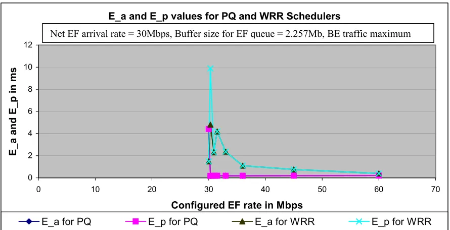
5.10.1.SUGGESTED VALUES OF E_A AND E_P... 68
5.10.2.CONCLUSIONS FOR EXPERIMENT 5 ON EFPHB... 69
5.11.EXPERIMENT 6 ON DBPHB ... 70
5.11.1.SUGGESTED VALUES OF SCORE S... 71
5.11.2.CONCLUSIONS FOR EXPERIMENT 6 ON DBPHB... 71
5.12.CASE STUDY OF THE EFPDB ... 72
5.12.1.OBJECT OF THE EFPDBCASE STUDY... 72
5.12.2.NETWORK TOPOLOGY FOR THE EFPDBCASE STUDY... 72
5.12.3.EXPERIMENT 1 ON EFPDB ... 74
5.12.4.EXPERIMENT 2 ON EFPDB ... 74
5.12.5.EFPDBCASE STUDY SPECIFICS... 74
5.12.6.DETAILS OF EXPERIMENT 1 AND 2 ON THE EFPDB ... 74
5.12.7.TOOLS USED FOR ANALYSIS... 75
5.12.8.RECORD OF RESULTS FROM EFPDBCASE STUDY... 75
5.12.8.1.RESULTS FOR PACKET LOSS... 75
5.12.8.1.1.OBSERVATIONS ON PACKET LOSS... 76
5.12.8.2.RESULTS FOR END-TO-END DELAY AND JITTER STATISTICS... 77
5.12.8.2.1.OBSERVATIONS ON END-TO-END DELAY AND JITTER STATISTICS... 78
5.12.9.CONCLUSIONS OF THE EFPDBCASE STUDY... 79
6. CONCLUSIONS ... 80
6.1.AREAS OF FUTURE RESEARCH... 82
7. REFERENCES... 83
8. APPENDIX... 86
APPENDIX A... 86
List of Tables
Table 1: Tabulation of Codec Specifications... 39
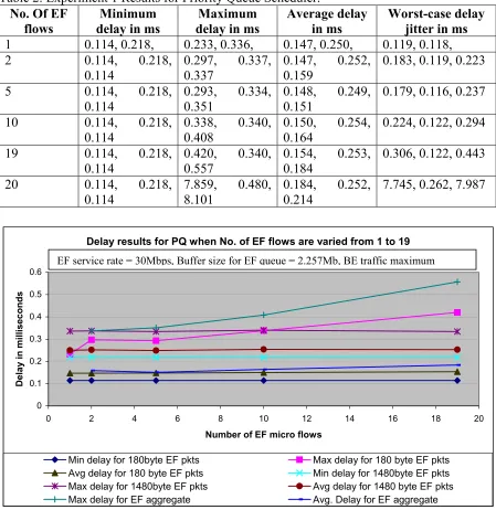
Table 2: Experiment 1 Results for Priority Queue Scheduler... 43
Table 3: Experiment 1 Results for Weighted Round Robin Scheduler. ... 45
Table 4: Experiment 2 Results for Priority Queue Scheduler... 51
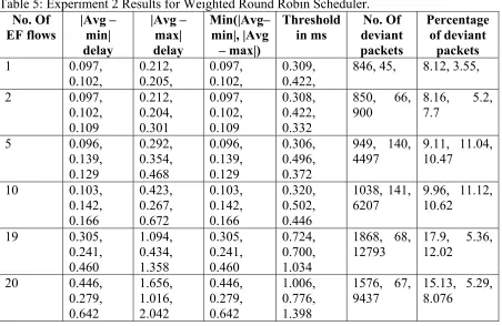
Table 5: Experiment 2 Results for Weighted Round Robin Scheduler. ... 51
Table 6: Variance and Standard Deviation in Packet Delay when number of flows is varied. ... 52
Table 7: 95 and 99 Percentile Per Hop Packet Delay for Priority Queue Scheduler... 54
Table 8: 95 and 99 Percentile Per Hop Packet Delay for Weighted Round Robin Scheduler. ... 55
Table 9: Experiment 3 Results for Priority Queue Scheduler... 57
Table 10: Experiment 3 Results for Weighted Round Robin Scheduler. ... 60
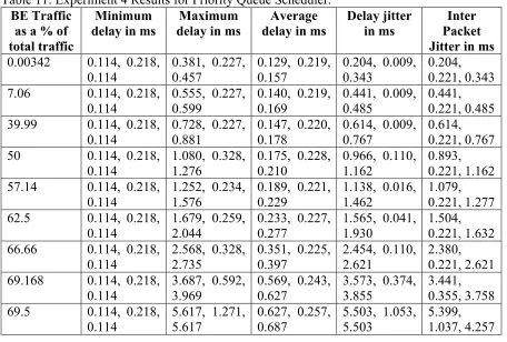
Table 11: Experiment 4 Results for Priority Queue Scheduler... 63
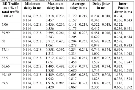
Table 12: Experiment 4 Results for Weighted Round Robin Scheduler. ... 65
Table 13: Experiment 5 Results for E_a and E_p... 68
Table 14: Experiment 6 Results for possible values for Score, S... 71
Table 15: Congestion Points for EF PDB Case Study... 75
List of Figures
Figure 1: Definition of the Differentiated Services Codepoint in the Ipv4 TOS Field... 11
Figure 2: Sample Topology used to illustrate the working of the DSA... 13
Figure 3: Block Diagram of the Classifier and the Traffic Conditioner within a DS Node. .. 16
Figure 4: Topology used for Experiments 1 – 6, consisting of 6 Sources, S1 – S6, 3 Sinks D1 –D3, 3 Edge Routers E1 - E3 and 2 Core Routers C1 - C2. ... 38
Figure 5: Minimum, maximum and average per hop delays plotted for PQ for micro-flow of small packets, large packets & EF aggregate when EF flows are varied from 1 to 19... 43
Figure 6: Minimum, maximum and average per hop delays plotted for PQ for micro-flow of small packets, large packets & EF aggregate when EF flows are varied from 1 to 20... 44
Figure 7: Delay jitter plotted for PQ for micro-flow of small packets, large packets and the EF aggregate when EF flows are varied from 1 to 19. ... 44
Figure 8: Delay jitter plotted for PQ for micro-flow of small packets, large packets and the EF aggregate when EF flows are varied from 1 to 20. ... 45
Figure 9: Minimum, maximum and average delays plotted for WRR for micro-flow of small packets, large packets and EF aggregate when EF flows are varied from 1 to 20... 46
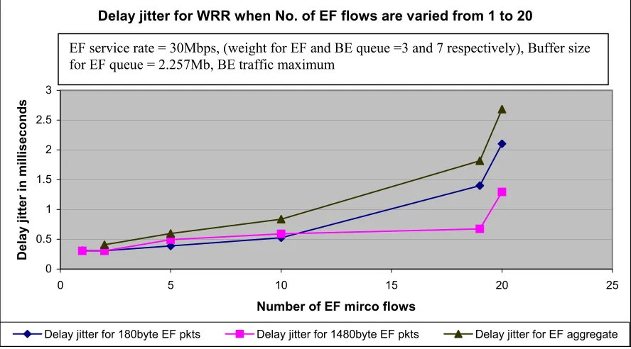
Figure 10: Delay jitter plotted for WRR for micro-flow of small packets, large packets and the EF aggregate when EF flows are varied from 1 to 20. ... 46
Figure 11: Standard deviation in per hop packet delay when number of EF flows is varied. 53 Figure 12: Delay report for PQ when ratio of EF arrival to departure rate is varied from 1 to 2 ... 58
Figure 13: Delay report for PQ when ratio of EF arrival to departure rate is varied from 1.01 to 2 ... 58
Figure 14: Jitter statistics for PQ when the ratio of EF arrival to departure rate is varied from 1 to 2 ... 59
Figure 15: Jitter statistics for PQ when the ratio of EF arrival to departure rate is varied from 1.01 to 2. ... 59
Figure 16: Delay report for WRR when the ratio of EF arrival to departure rate is varied from 1 to 2. ... 61
Figure 17: Jitter statistics for WRR when the ratio of EF arrival to departure rate is varied from 1 to 2... 61
Figure 18: Delay report for PQ when the net BE traffic is varied. ... 64
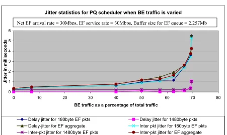
Figure 19: Jitter statistics for PQ when the net BE traffic is varied. ... 64
Figure 20: Delay report for WRR when the net BE traffic is varied. ... 65
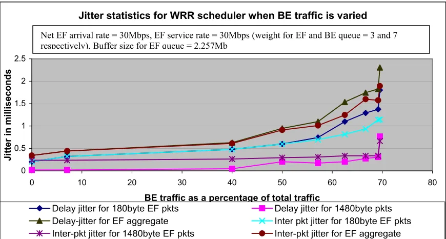
Figure 21: Jitter statistics for WRR when the net BE traffic is varied. ... 66
Figure 22: Calculated values of E_a and E_p for PQ and WRR. ... 69
Figure 23: Score S for DB PHB, when DB aggregate input rate is varied... 71
Figure 24: Network topology used for studying EF PDB Case Study ... 73
Figure 25: Packet loss for the EF PDB Case Study... 76
Figure 26: Delay statistics for EF PDB Case Study. ... 78
Figure 27: Delay jitter statistics for EF PDB Case Study... 78
Figure 28: Histogram 1 ... 86
Figure 30: Histogram 3 ... 86
Figure 31: Histogram 4 ... 87
Figure 32: Histogram 5 ... 87
Figure 33: Histogram 6 ... 87
Figure 34: Histogram 7 ... 88
Figure 35: Histogram 8 ... 88
Figure 36: Histogram 9 ... 88
Figure 37: Histogram 10 ... 89
Figure 38: Histogram 11 ... 89
Figure 39: Histogram 12 ... 89
Figure 40: Histogram 13 ... 90
Figure 41: Histogram 14 ... 90
Figure 42: Histogram 15 ... 90
Figure 43: Histogram 16 ... 91
Figure 44: Histogram 17 ... 91
Figure 45: Histogram 18 ... 91
Figure 46: Histogram 19 ... 92
Figure 47: Histogram 20 ... 92
Figure 48: Histogram 21 ... 92
Figure 49: Histogram 22 ... 93
Figure 50: Histogram 23 ... 93
Figure 51: Histogram 24 ... 93
Figure 52: Histogram 25 ... 94
Figure 53: Histogram 26 ... 94
Figure 54: Histogram 27 ... 94
Figure 55: Histogram 28 ... 95
Figure 56: Histogram 29 ... 95
Figure 57: Histogram 30 ... 95
Figure 58: Histogram 31 ... 96
Figure 59: Histogram 32 ... 96
Figure 60: Histogram 33 ... 96
1. Introduction
1.1. Motivation and Goals
The Internet was primarily designed to support best effort (BE) traffic. Unfortunately, it is not anymore constrained to just data traffic. The earlier specifications on which the Internet was built no longer apply. The growth of the Internet has fuelled the growth of data intensive media transmission, such as real time voice and video transmission. A number of new applications being developed for the Internet require stringent bounds on parameters such as the end-to-end delays and inter-packet jitter. In order to provide these bounds, there is a need for special Quality of Service (QoS) mechanisms. The Internet Protocol (IP), version 4, (Ipv4) by itself does not provide for a lot of flexibility as far as Quality of Service is concerned. This led to the development of alternate mechanisms based on policies that could be deployed on the existing network infrastructure with minimal changes, and still provide a suitable Quality of Service.
Differentiated Services (DS) is one such technology [1][2]. Aside from plain over-provisioning, DS is probably the most promising technology that can be implemented with relatively small disturbance to the existing infrastructure. Service Providers charge extra for services developed using service differentiation. One such service, Expedited Forwarding (EF) Per Hop Behavior (PHB) is of special interest since it is intended to have the most stringent QoS guarantees [4][7][8], and hence is most suitable for support of QoS sensitive applications. This thesis provides an analysis of some of the issues that arise in the EF PHB implementation, as well as in the application of that solution across a networking domain, i.e., it’s Per Domain Behavior (PDB). This is deemed important as the premium EF service can be provided to customers only if the EF service has been optimally configured within the DS.
1.2. Open Issues
a) Detailed characterization of the EF PHB based on different scheduling mechanisms and policers [2][4][7][8][12].
b) Benchmarking of various DS mechanisms and provision of a guideline for implementers [1][2].
c) Definition of appropriate values of QoS metrics that could be used by service providers while defining Service Level Agreements1 for commercial use [2].
d) Study of alternative QoS metrics for quantification of the QoS provided to the EF aggregate [12]. Study of the merit factors that characterize EF compliant DS nodes [7][8][9][12].
e) Study of the impact of buffer sizes as applied to the EF PDB where the amount of BE cross-traffic2 as well as other EF traffic in the core network, may violate the EF PHB [2][7][8][13].
1.3. Specific Issues Addressed in this Thesis
Characterization of the EF PHB based on the QoS metrics, such as minimum, maximum and average per hop packet delays, delay jitter, and inter-packet jitter experienced by packets within the EF aggregate are of special interest when it comes to jitter sensitive applications such as video and voice-over IP. Interactive video has the most stringent QoS requirement, with a data loss ratio requirement of 1x10⁻⁹ packets and a delay requirement of 500µs per switching node. Voice applications are more tolerant to loss, but less tolerant to delay with a loss ratio requirement of 1x10⁻⁶ and a delay requirement of 500µs per switching node [28]. Studies have also shown voice to be tolerant to end-to-end delays of as large as 150ms without causing any significant degradation in conversational dynamics [29]. Since these applications are of special interest to the end user community, the study of parameters governing the QoS provided by the EF service has been the main motivation behind this thesis. Ideally the EF PHB was defined such that EF traffic would spend very less time in queues, awaiting service within DS nodes. This in effect would provide a virtual leased line
service to the traffic flow [4]. This thesis aims at analyzing how various factors influence the queuing delay encountered by EF traffic within DS nodes.
Significance of measured parameters in the analysis: The minimum and maximum per hop delays provide the fixed delay and the total delay3 that a packet would encounter in a DS node. The delay jitter, which is the difference between the maximum and minimum delay, provides the variable delay a packet encounters in the DS node. This variable delay can be equated to the queuing delay experienced by packets within a DS node, which we are trying to minimize in DS. The extent to which we can reduce the queuing delay would determine the efficiency of a DS implementation. The inter-packet jitter provides an estimate to design the de-jitter buffers at the end destinations for streaming media applications.
Simulation techniques were used for running the experiments in this thesis, as several configuration parameters within the DS domains could be varied with considerable ease in order to run multiple scenarios of the same experiment. The simulation environment also permitted the study of topologies, especially for the EF PDB, which would not have been possible to set up due to limited resources. Details of the simulation environment are explained in Chapter 4. of this thesis.
Assumptions made in the Experiments: Several assumptions were made while designing the experiments in this thesis. All the DS nodes used in the experiments used the default implementation of a DS node within the simulator. Specific details regarding the internal architecture, the number of stages etc, were not accounted for in the simulations, as these would be vendor specific. All the DS nodes were assumed to be identical. This was a limitation in the analysis, as practically, DS nodes from various vendors with differing capabilities, will be employed in the networks. For the sake of simplicity, all the links were assumed to be Fast Ethernet links, while practically, multiple data link technologies are employed in the Internet. This was another limitation of this analysis. In practical networks, there is a possibility that packet loss occurs due to packet corruption during packet
forwarding and transmission, but this was not accounted for in the experiments as the probability of packet loss due to data corruption in today’s high-speed networks was considered to be very small, with a bit error rate of the order of 10-11 for Fast Ethernet [30]. The simulation time was restricted to 10seconds, as a single simulation run for this time duration could generate trace files of sizes up to 2Gb depending upon the number of packets transmitted in simulation time. Processing these trace files for relevant details was a time consuming task. Running the simulations any longer would result in even larger trace files. Running the simulations or observing similar practical implementations over a longer duration can result in an increase in the monitored parameters. Further the packets within the EF queue was assumed to be served in first in first out (FIFO) order. Practical implementations may use complex non-FIFO scheduling mechanisms within the EF queue depending upon the specific services and applications running on the DS networks.
The effects on individual micro-flows along with the EF aggregate comprising of these micro-flows were to be determined. As each of them would receive different QoS due to the presence of other EF micro-flows having different traffic characteristics and competing for the same resources, the QoS cannot be generalized. Hence analysis was made for:
a) A single EF micro-flow consisting of small packets within the EF aggregate. b) A single EF micro-flow consisting of large packets within the EF aggregate. c) The EF aggregate as a whole.
Determination of the small and large packet sizes is explained in Section 5.3. of this thesis.
A Comparative study of a Priority Queue scheduler and a Weighted Round Robin scheduler was done, when used with a Token Bucket policer to implement the EF PHB in a DS node, in order to provide norms for benchmarking other schedulers. This study was made for all the 3 cases mentioned above and consists of the following:
a) Effect of variation in the number of EF micro-flows and hence the net EF arrival rate for an output interface on the QoS metrics, to study effects of EF micro-flow aggregation and packet clustering.
threshold as a metric to quantify these delays, in order to provide a measure of confidence in providing the EF PHB.
c) Study of the effect of varying the net EF departure rate on a specific outgoing interface, when the net EF arrival rate was maintained constant, in order to determine the extent of over provisioning of resources, necessary to support EF traffic.
d) Study of the effect of variation in best effort cross-traffic in the network on the EF PHB to determine how traffic mapping to other PHBs, affect the EF PHB.
e) Study of the merit factors E_a and E_p when the EF configured rate for an output interface was varied [7], to study the range of possible values as compared to the delay jitter.
f) Study of the possible values of score S for the Delay Bound PHB [9] when the net arrival rate of DB traffic for an output interface was varied, to study the range of possible values.
A Case study of the EF PDB for studying the impact of cross-traffic on the EF traffic traversing consecutive DS domains, governed by common Service Level Agreements, thus creating a DS region was also done.
1.4. Thesis Layout
2. Differentiated Services Architecture
2.1. Definitions used in this Thesis [1][2]
Some of the terms used in the Differentiated Services Architecture are defined below:
Behavior Aggregate (BA) Collection of packets having the same DS codepoint and crossing a link in one direction.
Differentiated Services Domain (DS Domain)
A DS domain is defined as a contiguous portion of the Internet consisting of edge and core DS routers that are governed by a consistent set of policies and administered in a coordinated manner [1]. Multiple autonomous networks can be aggregated to form a single DS domain provided they are administered by a single entity.
Differentiated Services Region (DS Region)
Set of contiguous DS domains offering service differentiation over paths through those domains [2].
Micro-Flow A single instance of an application-to-application flow of packets identified by their source and destination address and port numbers [1].
Per Hop Behavior (PHB) A description of the externally observable forwarding treatment applied at the Differentiated Services-compliant node to a Behavior Aggregate.
Service Level Agreement (SLA) A service contract between either, a customer and a service provider or between two service providers specifying the forwarding service a customer should receive.
Services The overall forwarding treatment given to a particular traffic flow in one direction across a DS domain in accordance with a service level agreement.
Traffic Conditioning Defined as the control functions such as marking, monitoring, policing and shaping applied to a Behavior Aggregate in order to make it compliant with the Service Level Agreement.
2.2. Models for Service Differentiation
2.2.1. Relative Priority Marking Model
The Ipv4 “precedence field”4 is an example of a relative priority marking model implementation where the application, host, or proxy node selects a relative priority or precedence for a packet [2][31][38]. The network nodes along the path between the source and the destination examine the priority value within the packet’s IP header and apply the appropriate priority forwarding behavior.
The IP precedence field consists of bits 0-2, and it is a subfield of the IPv4 Type of Service (TOS) octet. The values that the three-bit IP precedence field might take, are assigned to various uses, including network control traffic, routing traffic, and various levels of privilege. The least level of privilege is considered to be routine best effort traffic. Some routers exist that use the IP precedence field to select different per-hop forwarding treatments [1][33][34]. Although early BBN IMP packet switches dating back to the late 1960’s implemented the precedence feature, early commercial routers and UNIX IP forwarding code generally did not [1]. As networks became more complex and customer requirements grew, commercial router vendors developed ways to implement various kinds of queuing services, including priority queuing, to handle the policies encoded in the precedence bits.
Routers using the priority model examine the IP addresses, the IP protocol numbers, the Transmission Control Protocol (TCP) or User Datagram Protocol (UDP) port numbers, and possibly some other header fields.
However, the specifications of the packet forwarding treatments selected by the IP precedence field are not specific enough for predictable differentiated services. A scalable architecture for service differentiation must specify the packet forwarding treatments in much more depth.
2.2.2. Service Marking Model
The IPv4 Type of Service (TOS) bits (bits 0-3) within the TOS octet are an example of a somewhat more detailed service marking model. Each packet is marked for a type of service, which could be minimize delay, maximize throughput, maximize reliability and minimize monetary cost [31][38]. Network nodes may select routing paths or forwarding behaviors, which are suitably engineered to satisfy these service requests [2].
There are two problems with this model:
• Since only 4 of the 8 bits in the TOS octet of the Ipv4 header are used as the significant TOS bits, only 16 different services can be provided.
• The model is applied on a per packet basis, and hence services applying to a sequence of packets cannot be applied here.
2.2.3. Label Switching Model
Multi Protocol Label Switching (MPLS) is an example of the label-switching model [25]. This model is state based and maintains state of traffic streams on all the nodes in the traffic path. Packets are classified into flows. At the ingress of such a network, each flow is associated with a Label Switched Path (LSP), and packets using this LSP are tagged with a forwarding label that is used for determining the next hop and the QoS to be delivered to this packet [26]. Technically, extremely fine granularity of resource allocation can be given to the flows as labels have only local significance. Traffic engineering and management can also be achieved by routing traffic via specific paths where multiple paths exist between two nodes within the network [24].
2.2.4. Integrated Services / Resource Reservation Protocol Model
The Integrated Services (Intserv)/Resource Reservation Protocol (RSVP) model uses path establishment, maintenance and teardown signaling mechanisms to control data flows directly at the path nodes. Packet classification and forwarding state is retained on each node along the data path. The Intserv / RSVP model relies upon traditional datagram forwarding in the default case, but allows sources and receivers to exchange signaling messages which establish additional packet classification and forwarding states on each node along the path between them [17]. This technique works with classical IP solutions, but does require extra code on the routing nodes.
A drawback is the absence of state aggregation. The number of states on each node scales in proportion to the number of concurrent reservations. The latter can grow to a very large number in large networks. Another drawback is the need for change in the application programming interfaces in order to support the RSVP signaling protocol.
The differentiated services mechanisms could be utilized to aggregate Intserv / RSVP state in the core of the network [35]. However, it is claimed that although the support of large number of classifier rules and forwarding policies may be computationally feasible, the management burden associated with installing and maintaining these rules on each node within a backbone network that will be traversed by a traffic stream is substantial [2].
2.2.5. Static Per Hop Classification Model
In this model, static classification and forwarding policies are implemented at each hop (router) along the network. These policies are not updated based on the active state of the network but on a periodic basis.
updates, and as these periods can be long, static networks may result in substantial down time.
2.3. The Differentiated Services Architecture Model
Differentiated Services Architecture (DSA) model tries to address most of the problems brought up in the previous section. Traffic entering a Differentiated Services network is classified and conditioned at the DS ingress node according to pre-defined Service Level Agreements and accordingly assigned to a behavior aggregate. A codepoint uniquely identifies each behavior aggregate. This codepoint determines per hop forwarding treatment meted out to the packet in the core of the network. In other words, the DSA provides QoS by dividing traffic into different categories, marking each packet with a codepoint that indicates its category, and scheduling packets according to their codepoints.
This model has a number of advantages in comparison with the previously mentioned models. They include:
• The state of independent traffic flows need not be maintained within the network. • No direct signaling mechanisms are required for setting up, maintaining and tearing
down paths within the network, thus core nodes are not burdened, and no extra network bandwidth is spent on account of these mechanisms. However, policies still have to be defined on each node, and a mechanism needs to exist to do that.
• Applications can be unaware of this model and still use its services.
• A finer granularity of forwarding treatment can be given to packets than that offered by the Ipv4 precedence field or the Ipv4 type of service field, specifically one can have as many as 64 distinct forwarding treatments as 6 bits are used for the codepoint. • QoS can be provided without changing the network infrastructure, except for the need
to install DS capabilities on the network nodes.
• The implementation can be incremental and can coexist with non-differentiated services networks.
2.3.1. The Differentiated Services Field Definition [1]
1 2 3 4 5 6 7 8
DSCP Currently Unused
Figure 1: Definition of the Differentiated Services Codepoint in the Ipv4 TOS Field
Six bits of the Ipv4 TOS octet are used as a Differentiated Services Codepoint5 (DSCP) to select the PHB a packet experiences at each DS node, resulting in 64 distinct codepoints. DS compliant nodes when determining the PHB to apply to a received packet ignore the value of the Currently Unused (CU) bits. The entire 6-bit DSCP field must be used by DS compliant nodes while mapping a packet belonging to a behavioral aggregate to a particular PHB.
2.3.2. Backward Compatibility with IP Precedence Field [1]
In order to maintain backward compatibility with the IP precedence field, a set of codepoints called Class Selector Codepoints mapping to PHBs have been defined that are compatible with the forwarding treatments selected by the IP Precedence Field. These Class Selector Codepoints may map to PHBs. The minimum requirements for these PHBs are called the Class Selector PHB requirements [1]. A specification of the packet forwarding treatments selected by the DSCP with a value of ‘xxx000’ and Currently Unused (CU) subfield unspecified, are reserved as a set of eight Class Selector Codepoints [1]. PHBs mapping to these codepoints must satisfy the Class Selector PHB requirements in addition to preserving the Default PHB requirement on codepoint ‘000000’ [1]. As the Ipv4 Precedence marking is a relative priority model, a Class Selector Codepoint with a higher numerical value has a higher relative order than one with a lower numerical value. At least two independently forwarded classes of traffic must be provided by the set of PHBs mapped to by the eight Class Selector Codepoints. The Ipv4 Precedence field assigns values ‘110’ and ‘111’ for routing traffic. Hence a preferential forwarding treatment must be given by PHBs selected by codepoints ‘11x000’ in comparison to the PHB selected by codepoint ‘000000’.
2.3.3. Some details
The Differentiated Services Architecture (DSA) is based on the simple concept of classifying packets at the network boundaries and marking these packets with appropriate codepoints based on the rules of the administrative policies, conditioning these packets in conformance with the policies, and giving these packets a forwarding treatment corresponding to their classification in one direction of propagation. Flow aggregation in the core is an important concept in DSA that aids in scaling this technology to large networks. Scalability is achieved by considering individual traffic micro-flows arriving at the edge DS nodes, and by aggregating them into well-defined traffic aggregates based on the codepoint to PHB mapping. These traffic aggregates are dealt with in the core of the DS Domain.
At the core, DS nodes are required to support mechanisms that classify, schedule and provide buffer management to packets for the appropriate forwarding treatment [1]. In addition, edge routers need to implement mechanisms to mark packets and condition them.
The DSA has two elements. The first concerns the mechanism of forwarding the packets. This includes the differential treatment given to a packet via scheduling and queuing mechanisms [1]. The forwarding path will also need to monitor packets for billing purposes and to ensure compliance of packets to the service agreements, and to police and shape the packets in the case they are not conforming to their service agreement. These functions are important to ensure that the service provider can actually provide the service promised to all customers. The second element is the setting of the node parameters that govern the packet forwarding process. This is an area where a lot of active research is being done.
Services are realized by the combination of traffic conditioning and marking at the ingress nodes of a DS network, along with the scheduling and queuing in the core DS nodes.
2.4. Operation of a Differentiated Services Network
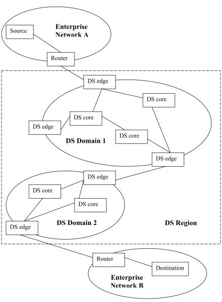
Figure 2: Sample Topology used to illustrate the working of the DSA. Source
Router
DS core DS edge
DS edge DS core
DS core
Enterprise
Network A
DS Domain 1
Router
Destination
Enterprise
Network B
DS core DS core
DS edge
DS edge
DS Domain 2
DS edgeTraffic originates as independent micro-flows at the source node within enterprise network A. This traffic is destined for a node within the enterprise network B. The boundary router within network A forwards the traffic to the ingress node, also called the edge node of DS domain 1. The edge node, depending upon the service level agreement existent between the service provider and the enterprise network A, classifies and marks the packet with a codepoint, conditions the traffic and assigns it to a per hop forwarding behavior. In the absence of a service level agreement all the traffic originating from Enterprise network A is considered best effort traffic and marked to the codepoint “000000”, which maps to the default PHB. The default PHB is not meant to provide any form of QoS guarantees to the traffic. It just forwards packets when resources are available.
Once this is done, core DS nodes only forward the packets based on the DS codepoint assigned to packets. The core nodes forward the traffic to the egress DS node, which ultimately either delivers the packets directly to the router within the enterprise B network if it is directly connected to it, or it forwards the packets to the ingress router of another DS domain. In the latter case it is the ingress router of DS domain 2. This process continues till a DS domain can directly deliver the packets to the enterprise network B. In this case the traffic is sent from one DS domain to another DS domain. The downstream DS domain, which is DS domain 2 in our case, is free to assign a different codepoint to this traffic as long as it maps it to an equivalent PHB.
Any packet received at the downstream DS domain with a codepoint that doesn’t map to any PHB in its PHB table is re-marked with the default codepoint of “000000” and treated as if it belonged to the default PHB.
micro-flows needs to be maintained within the core of the DS domain. Once the traffic reaches the edge of the DS domain, it can be de-aggregated and delivered to its respective locations.
In the Figure 2, the two consecutive DS domains form a DS region represented by the square dotted box surrounding them. This is because common traffic conditioning agreements are defined between these two DS domains to handle traffic through them.
2.5. Major Logical Components of a DS Node
A DS node can be considered to comprise of several DS elements. Depending upon whether the DS node is an edge node or a core node, the particular elements implemented can vary. The elements are:
• Packet Classifier • Traffic Conditioner • Buffer Manager • Scheduler
2.5.1. Packet Classifier
2.5.2. Traffic Conditioner
A traffic conditioner on receiving traffic flows from the packet classifier further processes the traffic by passing it through several sub modules listed below.
• Meter
• Packet Marker • Shaper
• Packet Dropper
The logical view of the Packet Classifier and Traffic Conditioner is shown in the Figure 3 below [2]:
Packets
Figure 3: Block Diagram of the Classifier and the Traffic Conditioner within a DS Node.
2.5.2.1. Meter
The meter uses the traffic conditioning agreement as a reference and measures the temporal properties of a traffic flow to determine whether a packet is within the specified profile or misbehaving [1]. Based on this measurement, signals are passed to the other sub-modules to trigger specific actions on the packet.
Meter
Shaper/
Dropper
Classifier
Marker
2.5.2.2. Packet Marker
Based on the traffic streams received from the classifier, the packet marker module maps the packet to a particular PHB and sets the DS field within the Ipv4 header to a specific DSCP. On the basis of this codepoint, DS core nodes will give it the appropriate forwarding treatment by using the codepoint as an index to the codepoint to PHB mapping table. Packet marker is a required module in DS edge nodes. For any traffic originating within the DS domain and requiring service differentiation, some internal DS core nodes will need to have the functionality of a packet marker, as they will need to mark the DSCP within the Ipv4 packet header.
2.5.2.3. Shaper
The shaper modifies the inter-packet times within a traffic stream in order to make it compliant with the traffic profile. This is necessary in case the traffic stream has been backlogged in the immediate upstream DS node behind other traffic, and as a result appears as a burst of packets to the input interface of the DS edge node.
2.5.2.4. Dropper
The dropper is responsible for dropping packets belonging to a traffic stream in order to make the traffic stream compliant with the service profile. This process is defined as “policing” a stream [2]. The dropper and shaper modules are closely related and implemented many a times as a single module.
2.5.3. Buffer Manager
prevent congestion by means of mechanisms like Random Early Detection (RED) by keeping the average queue size small but still permitting small bursts of packets to be serviced [23].
2.5.4. Packet Scheduler
A scheduler is used in order to provide sharing of network resources and providing certain traffic flows with performance guarantees. A packet scheduler determines which packet queue within a DS node will be served next based on the PHBs and the services built on those PHBs within the DS domain. The scheduler implemented within a DS node principally determines the performance that a PHB receives. Each scheduler is designed to satisfy one or more of the following requirements: ease of implementation, ease and efficiency of admission control, fairness and protection, and performance bounds which aid in bounding the QoS metrics.
2.6. Per Hop Behavior [2]
The Per Hop Behavior (PHB) is the means by which a DS compliant node allocates resources to behavior aggregates. Based on this basic resource allocation on each DS node within a DS domain, useful services can be constructed. Traffic characteristics associated with a behavior aggregate are responsible for the behavior of a PHB. Other PHBs may also influence the treatment given to packets by the PHB under consideration. A PHB can be specified by means of the resources allocated to it compared to other PHBs, or by means of measurable QoS metrics like packet loss, packet delay etc [2].
2.7. Per Domain Behavior [6]
Technically, the Per Domain Behavior6 (PDB) is defined as a building block that outlines the relationship between classifiers, traffic conditioners, specific PHBs and particular configurations with a resulting set of specific observable attributes that may be characterized in several ways [6]. A PDB is used to describe the forwarding behavior experienced by a traffic aggregate, as it crosses a DS domain. PDBs are characterized by specific metrics quantifying the treatment a set of packets with the same DS codepoint will receive as they cross the DS domain. PDBs are meant to help Internet Service Providers construct services based on the DSA. A PDB can be thought to comprise of two aspects. The first part is the traffic conditioning at the boundary nodes to form the traffic aggregate, and the second is the treatment this traffic aggregate experiences within the DS domain. PDBs are always specified over a known network topology, and cannot be generalized to any topology.
3. Expedited Forwarding Per Hop Behavior
This thesis focuses on the evaluation of some of the properties of the Expedited Forwarding (EF) PHB. Therefore, this chapter concentrates on describing this in more detail. EF PHB is defined for providing a low loss, low delay, low jitter and assured bandwidth end-to-end service through autonomous Differentiated Services Domains without per flow queuing [4].
The EF PHB is defined as a forwarding treatment for a particular DS aggregate where the departure rate7 of the aggregate’s packets from any interface of a DS node must exceed the arrival rate of the aggregate’s packets for that interface [4].
The Experiments 1 to 6 on the EF PHB deal with the characteristics delay, jitter and bandwidth. All these characteristics in addition to packet loss are considered for the EF PDB case study. Loss is not noted for the EF PHB experiments as all the analysis is done within a DS core node and no loss is observed at this node as the incoming EF traffic is already conditioned at the ingress DS node. Unless explicitly stated as inter-packet jitter, jitter for the EF PHB, is defined as the variation between the minimum and maximum delays and termed delay jitter [7].
3.1. EF PHB Codepoint
The EF PHB is assigned the codepoint ‘101110’ from the Standards Action pool [4]. This codepoint is marked at the ingress nodes of the DS domain. By definition, packets marked with the EF PHB will never be promoted or demoted to another PHB unlike the packets belonging to the AF PHB. EF traffic flows should be allowed to traverse multiple DS domains provided appropriate Service Level Agreements (SLAs) exist between every adjacent DS domain along the path of the traffic. However the absence of an SLA between two DS domains causes the ingress router of the downstream DS domain to drop the packets it receives from the upstream DS domain. This, of course, can be the source of problems and this factor has to be accounted for in any case study of the EF PDB.
3.2. Packet Delays Experienced by the EF PHB
Delay experienced by end-to-end transfer of packets can be attributed to at least five reasons: packetization delay, forwarding delay, queuing delay, serialization delay, and propagation delay.
Packetization delay is the duration of time at the sending host, that digital samples are held for placement into the packet payload until enough samples are collected to fill the packet payload.
Forwarding delay takes place in the sending host and the routers, and is the time taken to receive a packet, make a forwarding decision and then begin sending the packet on the outgoing interface.
Queuing delay is the delay experienced by a packet within routers and switches while waiting on packets that arrived before it to be serviced and sent on the outgoing interface. At any point in time a packet may be waiting in queue a variable amount of time while awaiting access to the output link. The instantaneous state of the router or switch decides the length of this delay.
Serialization delay occurs at the sending host and the intermediate routers, and is the time taken to physically put the bits of a packet on the wire when a node transmits a packet. Serialization depends upon the size of the packet and the speed of the output interface. It is not affected by the maximum EF configured rate for that interface. Serialization delay is always computed using the speed of the output interface.
We usually cannot control the forwarding delay, serialization delay, or propagation delay since they are properties of the hardware infrastructure, but we can usually try to control the queuing delay. The EF paradigm aims at reducing this queuing delay for EF traffic. Queuing delay in a well designed and properly functioning DS network can be several orders of magnitude less than the propagation delay. Further, policing and conditioning the traffic at the ingress DS nodes can result in bounding delay jitter, packet loss and the provision of assured bandwidth to EF traffic.
3.3. Characteristics
In order to provide the qualities namely low loss, delay and jitter, that are characteristic of the EF PHB, to a flow of traffic, this traffic should either experience no queues or should spend minimal amount of time in the queues inside the DS nodes. This is the only way delay and delay jitter can be bounded. We can ensure that packets marked for EF forwarding are routed through the network with the highest priority. Provided the DS network has been provisioned appropriately, none of the EF traffic queues will ever overflow, reducing packet loss to zero.
To provision a DS network to handle the EF traffic appropriately, and provide QoS guarantees, every node in the DS network supporting the EF PHB should be configured such that
a) The departure rate for this traffic flow in that node is higher than the maximum arrival rate, and
b) This traffic flow is appropriately isolated from other traffic flows belonging to other PHBs. (The latter could be AF and BE PHBs.)
limit us from doing this. The reason being, at 100 percent utilization8, as the node cannot receive a packet on its input interface and finish forwarding the packet on its output interface in zero time, the node will always be backlogged with at least one packet. The Experiment 3 on the EF PHB in this thesis clearly demonstrates this point.
The EF traffic flow should also be conditioned at the DS edge node that is the ingress into the DS domain, so that it will never exceed the configured EF departure rate in any node in the path of that traffic-flow within that DS domain. EF traffic in excess of the maximum EF configured rate cannot be policed to other codepoints, and should be dropped at the DS ingress edge router.
3.4. Selection of Schedulers to Implement EF PHB
The EF PHB could be implemented with any scheduler that provides priority to select the traffic. The simplest option is the Priority Queue (PQ) Scheduler with the EF aggregate assigned the highest priority up to an EF configured rate. In this case as long as there are EF packets to be forwarded in any DS node, other traffic will be queued up until the time when there is no more EF traffic to forward, and provided the EF traffic rate is less than the EF configured rate for that output interface in that DS node.
A Round Robin (RR) Scheduler is the simplest emulation of the Generalized Processor Sharing scheduling discipline, where instead of serving each packet queue in an infinitesimal time, all the packet queues are served in a finite amount of time [10]. However no priority exists within the RR scheduler and hence it cannot be directly used to implement the EF PHB. A modified Round Robin scheduler called the Weighted Round Robin (WRR) Scheduler can be used. It is the one in which integral weights are assigned to each of the packet queues and the queues are served in proportion to the weight assigned to them.
Most practical implementations of the EF PHB use a single high priority queue or a single high-weight queue in class based queuing schedulers [12]. One of the limitations of the WRR
schedulers is that the amount of data taken from a queue is based on the number and size of packets served from that queue in the measurement time. This limitation isn’t present in the PQ scheduler as a queue is given priority up to a certain bandwidth of the output link. These implementations also offer a high degree of scalability, with minimum complexity and hence are attractive options for implementing the EF PHB [12]. Hence, for the experiments on EF PHB discussed in this thesis, the PQ scheduler is compared with the WRR scheduler. Experiments 1 to 6 on the EF PHB in this thesis evaluate the PQ scheduler and the WRR scheduler, to determine the conditions and the extent to which one is better than the other for implementing the EF PHB.
3.5. Policing EF PHB
Just as the EF traffic flows need to be protected from other traffic, other traffic also needs to be protected from unconditioned EF traffic. A policer is used to condition the traffic at the DS ingress node in order to ensure that EF traffic is less than the maximum EF arrival rate contracted for in the SLA. If this is not done, the EF traffic flows could starve the traffic belonging to other PHBs by consuming all the resources. Conditioning is achieved with the help of a token bucket policer associated with the EF queue. The token bucket policer is the recommended way of implementing the EF PHB [4].
3.6. Redefinition of the EF PHB
The EF PHB was recently redefined by the IETF. It is now characterized with mathematical relationships [7]. This was done to formally define the timescale over which the configured EF rate should be measured. The earlier definition of the EF PHB was much more relaxed with respect to the timescales over which the measurements should be made [7][8]. Hence even measurements on a compliant EF stream (based on that definition) and carried over short intervals, could yield noncompliant results as proved in [12]. With short measurement periods, sampling errors may arise giving incorrect statistics. With longer measurement periods, an averaging effect will take place, and noncompliance in subsections of the measurement period may go undetected.
The new definition specifies that every DS node supporting the EF PHB must be characterized by
a) A maximum EF departure rate, and
b) Bounds on the deviation of the actual departure time from the ideal departure time of each packet [7][8].
This is done as follows. The EF behavior is now defined by two sets of equations. One set applies to the EF aggregate as a whole, and the other set applies to each individual EF packet. The following equations need to be satisfied on a DS node supporting EF PHB on an interface configured at a maximum rate R [7].
For an EF aggregate behavior as a whole:
Furthermore, F_j is defined by basic relationships f_0 = 0, d_0 = 0, and the recursion
F_j = max (A_j, min (d_j-1, f_j-1)) + L_j/R for all j >0 ____________________(2) Where, D_j = actual departure time of packet j, F_j = ideal departure time of packet j, A_j = arrival time of packet j, L_j = size of the jth packet in bits, R = maximum configured EF rate at output I in bits/second.
The second set of equations applies to each individual packet marked for EF forwarding: D_j <= F_j + E_p for all j >0 ____________________(3) Where, D_j = actual departure time of packet j, F_j = ideal departure time of packet j, E_p = error term for the treatment of individual EF packets. E_p represents the worst-case deviation between the actual and ideal departure time of an EF packet. Hence E_p provides an upper bound on (D_j – F_j) for all j.
Furthermore, F_j is defined by basis relationships f_0 = 0, d_0 = 0, and the recursion
F_j = max (A_j, min (d_j-1, f_j-1)) + L_j/R for all j >0 ____________________(4) Where, D_j = actual departure time of packet j, F_j = ideal departure time of packet j, A_j = arrival time of packet j, L_j = size of the jth packet in bits, R = maximum configured EF rate at output I in bits/second.
E_a and E_p are both expressed in units of time. The maximum EF configured rate R can be the line rate or less, and E_a and E_p can either be specified as a function of R or as a worst-case value for all possible values for R. E.g. for a 100Mbps output interface, R can be either 100Mbps or less and the E_a and E_p can either be specified at 10Mbps, 20Mbps etc or as a worst case value for all possible values of R.
this common value as E. Thus E_a = E_p = E. The relationship between this E and the delay jitter is explained in Section 3.6.5. of this thesis.
3.6.1 Measuring E_a
A method for measuring E_a is proposed here. The equations 1 and 2 explained in Section 3.6. of this thesis, can be implemented by maintaining, for each outgoing interface, a linked list of elements whose members are “the packet arrival time”. A unique linked list is maintained for each output interface. Whenever a packet is received, on any one of its input interfaces, destined for a specific output interface, the element is filled with the packet arrival time and added to the tail of the linked list belonging to this output interface. Whenever a packet is sent out of that particular interface, the departure time is noted and the arrival time from the element at the head of the linked list is retrieved and the E_a is calculated. The first time this computation is done, the E_a value is stored. For successive E_a computations, if the calculated E_a value is larger than the previously stored E_a value, the new value is stored. This is followed by the removal of the element at the head of the linked list. As no state of packets is maintained, this processing can be performed in real time.
A setup similar to the one described above, but using arrays in AWK scripts was used while measuring the E_a values from the data collected in trace files after a simulation run in this thesis. Sample E_a calculations are shown in Section 3.6.3. of this thesis.
3.6.2. Measuring E_p
the unique ID, to obtain the packet arrival time. The E_p can now be calculated. The first time this computation is done, the E_p value is stored. For successive E_p computations, if the calculated E_p value is larger than the previously stored E_p value, the new value is stored. This is followed by the removal of this structure from the linked list.
A setup similar to the one described above, but using arrays in AWK scripts was used while measuring the E_p values from the data collected in trace files after a simulation run in this thesis. Sample E_p calculations are shown in Section 3.6.3. of this thesis.
One issue is what happens when packet arrival is recorded, but the packet is, for some reason, dropped in the DS node. Its entry could remain in the linked list and provide incorrect results. Hence, in the case a packet is dropped, its member in the linked list must be removed, and this event must be logged. These events can be used for throughput and packet loss calculations. Thus the dropped EF packet does not contribute to the measurement of E_a and E_p of the EF traffic, as recommended by IETF [7]. E_a and E_p calculations are made only on packets that were successfully forwarded by the node. This was also the method adopted in the simulations in this thesis.
A drawback of measuring E_p in a real implementation using the technique explained above is that the processing time per packet in the node will increase. This will be because, on receiving a packet destined for a specific interface, its IP header will have to be read to extract the fields and to generate a unique ID for this packet. Again, while sending this packet, the fields from its IP header will have to be extracted to determine its unique ID. Searching the linked list to retrieve the structure belonging to this specific packet in the linked list will also add to the overhead. One way in which this overhead can be reduced is for the measurement and monitoring to happen by means of a periodic offline (asynchronous) test using previously collected data, rather than in real time.
intent of this thesis has been to implement the two sets of equations for E_a and E_p and to determine the general range of possible values of E_a and E_p that are possible in a DS node under certain conditions. The relation of the E_a and E_p terms to the delay jitter was also determined. A study of the possible values for R, which is the EF configured rate and the corresponding E_a and E_p values was determined in Experiment 5 on the EF PHB, where the two sets of equations governing E_a and E_p were applied to a network with a Priority Queue scheduler implementation and to a network with Weighted Round Robin scheduler implementation.
3.6.3. Sample Calculations
Considering the EF aggregate is served in FIFO order (i.e. E_a = E_p = E) at a DS node, and considering we begin measurement at time zero. Let the speed of the output link be 100Mbps. Let the EF configured rate at the DS node be 33Mbps. Let the arrival time, A_1, of the first IP packet since the start of measurement at the DS node be 0.250ms from the start of measurement and its size, L_1, be 200bytes (including IP header) which is equal to 1600bits. Applying the equations 1 and 2, and considering f_0 = 0 and d_0 = 0, we get, the ideal departure time F_1 = max (A_1, min (d_0, f_0)) + L_1 / R = 0.298ms. The actual departure time D_1 is 0.365ms. The error term E = (D_1 – F_1) = 0.067ms. The largest value of E observed over the measurement period will provide us with the worst-case value of E.
3.6.4. Figures of Merit
E_a and E_p can be considered as figures of merit of a device [7]. A smaller value of E_a signifies a smoother service rate (scheduling) for the EF traffic flows over short timescales, while a larger value signifies a burstier scheduler whose steady-state properties will hold only over longer timescales. It is preferable to have a smaller E_a. A device with a smaller E_a will conform to the EF PHB over both shorter and longer timescales.
normally if EF packets arrive simultaneously on more than one input interface around the same time, and are destined for the same output interface. In that case the node can use a scheme to break up the tie between these packets and queue them accordingly. Depending on the order in which the packets are queued, some of them will experience greater delays than others. E_a will always be lesser than E_p in case of a non FIFO EF queue or equal to E_p in case of FIFO EF queue.
3.6.5. Delay and Jitter [7][8]
Assuming that the EF aggregate is served in FIFO order at a DS node (i.e. E_a = E_p = E), the per hop delay can be calculated from the formula
D_t = Q_t/R + E _____________ (5) Where, D_t is the per hop delay of an EF packet arriving at time t,
R = maximum configured EF rate at output interface in bits/second And Q_t is size of the EF queue in bits at time t
As an EF packet may be sent out as soon as it is received, the minimum delay through the node, Dmin, can be found by determining the fixed delay through the node. The maximum D_t observed for EF packets over the period of measurement at a DS node is the maximum value of per hop delay called Dmax. The difference between Dmax and Dmin will provide an upper bound on the delay jitter.
3.7. The Delay Bound PHB
The earlier definition of the EF PHB led to the definition of a new PHB called Delay Bound (DB) PHB, which has properties similar to EF PHB, but provides a strict bound on the delay variation (delay jitter) of conformant packets through a node [4][9]. The reasoning behind this definition is that the difference in time between when a packet might have been delivered, and when it is delivered, will never exceed a specifiable bound [9].
D_i – E_i <= S * MTU/A __________________ (6) Where, D_i = actual time a DB packet is delivered. This can also be considered as the time a packet will be delivered in the presence of competing traffic.
E_i = ideal time a DB packet should be delivered. This can also be considered as the time a packet will be delivered in the absence of competing traffic.
A = net arrival rate of DB traffic at the node for the specific output interface. MTU = maximum transmission unit in bits for the output interface.
S = a constant called score that is a characteristic of the device at rate A.
The score is dependant on the scheduling mechanism and configuration of the device.
Experiment 6 on the EF PHB in this thesis used the equation 6 to determine the range of values of A and their corresponding S values.
3.7.1. Codepoint for the DB PHB
The codepoint used for the DB PHB is ‘101111’ and comes from the Experimental pool of codepoints [9]. The EF PHB, in comparison uses a codepoint of ‘101110’ from the Standards Action pool of codepoints. One thing to note is that any codepoint of the form ‘xxxxx0’ comes from the Standards action pool of DSCP (e.g. the EF PHB codepoint) while any codepoint of the form ‘xxxxx1’ comes from the Experimental or Local Use pool of DSCP.
3.7.2. Jitter for DB PHB
4. Tools and Methods
4.1. Simulation Environment
All the simulations for this thesis were run on the Network Simulator (ns-2) version2, beta release 6 and beta release 8. The simulator was implemented on two SUN ULTRA10 SPARC workstations running the Solaris 7 operating system.
4.2. Network Simulator ns-2
Ns-2 is a freely available discrete event simulator targeted at networking research. A number of organizations are performing research on improving and contributing modules to the simulator. The University of Southern California primarily maintains the source code for the simulator. Ns-2 provides substantial support for simulation of TCP, UDP, multicast and routing protocols over wired and wireless (local and satellite) networks [19].
4.2.1. Limitations of ns-2
Ns-2 is not a polished and finished product, but the result of an on-going effort of research and development. In particular, bugs in the software are still being discovered and corrected. It is entirely the responsibility of the user to validate the results generated by the use of the simulator.
4.2.2. Characteristics of ns-2
hierarchy is automatically established through methods defined in the class TclClass. User instantiated objects are mirrored through methods defined in the class TclObject. There are other hierarchies in the C++ code and OTcl scripts that are not mirrored in the manner of TclObject.
4.2.3. Need for Split Language Programming
Systems programming is required for the simulation of communication protocols where access to, and manipulation of packet headers and bytes is possible. These protocols should be able to run over large data sets to appropriately model the algorithms and generate sufficient information from which results can be derived with an acceptable degree of confidence. All these above mentioned tasks make run-time speed an important criterion.
The C++ programming language is chosen for the task of implementing algorithms and protocols, as it can be designed in a modular manner allowing individual contributors to provide small sections of the simulator. Running the executable code of a compiled C++ package is very time efficient.
The other task of any simulation involves fine-tuning and varying the parameters used for successive simulation runs. Sometimes it is important to vary the configurations marginally and study the performance. For all these tasks, if we had to make changes to the C++ program, it will be a very time consuming job. There is also the chance of unknowingly modifying a section of the source code of the algorithms, which can ultimately lead to simulation results that can’t be accounted for, invalidating the entire simulation. For all these reasons, the time required to change the parameters and start the next run becomes important. OTcl is chosen for this task. As it is an interpreted language, it does not need to be compiled after making changes to the simulation scripts.
4.2.4. Usage of Languages
Development of newer modules for the simulator in order to implement newer protocols and algorithms or to improve or extend the behavior of existing modules requires the use of the C++ language. The entire package will have to be recompiled after the changes are made, to actually make the changes take effect for a simulation run. Writing simulations based on the features and behaviors of algorithms and protocols already implemented in ns-2 requires the use of the OTcl language.
An example is: Links are OTcl objects that assemble delay, queuing, and possibly loss modules [19]. If we can design our simulations with these objects, then only OTcl needs to be used. On the other hand the implementation of a special queuing, or scheduling mechanism will warrant the use of the C++ language.
4.3. Overview of the Differentiated Services Module in ns-2
The Advanced IP Networks group in Nortel Networks originally developed the Differentiated Services module for ns-2. This very same module was integrated into the network simulator, version 2, Beta release 8.
4.3.1. Major Components of the Differentiated Services Module [20]
“Three major components comprise the Differentiated services module:
• Policy: Policy is specified by network administrator about the level of service a class of traffic should receive in the network.
• Edge routers: Edge routers marks packets with a codepoint according to the policy specified.
• Core routers: Core routers examine the packets codepoint marking and forward them accordingly.
Diffserv attempts to restrict complexity only to the edge routers.”
4.3.2. RED Queue for Diffserv [20]
“In ns, the Diffserv functionality is captured in a Queue object, which is implemented as an alternative to other queue types such as DropTail, CBQ, and RED. A Diffserv queue contains the abilities:
1. to implement multiple physical RED queues along a single link;
2. to implement multiple virtual queues within a physical queue, with individual set of parameters for each virtual queue;
3. to determine in which physical and virtual queue a packet is enqueued, according to policy specified.
Instead, it is a modified copy of that class that includes the notion of virtual queues. Instances of the REDQueue class only exist inside instances of the dsREDQueue class. All user interaction with the REDQueue class is handled through the command interface of the dsREDQueue class. The dsREDQueue class contains a data structure known as the Per Hop Behavior Table (PHB Table). Edge devices handle marking packets with codepoints and core devices simply respond to existing codepoints. However, both devices need to determine how to map a codepoint to a particular queue and precedence level. The PHB Table handles this mapping by defining an array with three fields:
struct phbParam {
int codePt_; // corresponding codepoint int queue_; // physical queue
int prec_; // virtual queue (drop precedence) };”
4.3.3. Policy [20]
policer type, a meter type, an initial codepoint, and other state information. The Policy class uses a Policer Table to store the mappings from a policy type and initial codepoint pair to its associated downgraded codepoint(s).
Currently, six different policy models are defined, which are:
1. TSW2CM (TSW2CMPolicer): uses CIR and two drop precedences. The lower precedence is used probabilistically when the CIR is exceeded.
2. TSW3CM (TSW3CMPolicer): uses CIR, PIR, and three drop precedences. The medium drop precedence is used probabilistically when the CIR is exceeded and the lowest drop precedence is used probabilistically when the PIR is exceeded.
3. Token Bucket (tokenBucketPolicer): uses CIR and CBS and two drop precedences. An arriving packet is marked with the lower precedence if and only if it is larger than the token bucket.
4. Single Rate Three Color Marker (srTCMPolicer): uses CIR, CBS, and an EBS to choose from three drop precedences.