ABSTRACT
OH, SAEBITNA. Significance Tests for Longitudinal Functional Data. (Under the direction of Ana-Maria Staicu and Arnab Maity).
Longitudinal functional data consist of functional samples, e.g. profiles or images, observed
for each of many subjects at multiple repeated instances (e.g. day). Main challenge in
longitudi-nal functiolongitudi-nal data alongitudi-nalysis is the complex dependence structure induced by within-function and
between-function correlations. This thesis aims to develop novel inferential methodologies to address
common scientific questions in longitudinal functional data.
In the first part of the thesis, we develop inferential approaches to study the association
be-tween one-dimensional functional response and scalar covariates in longitudinal functional data.
Our main objective is to study the covariate effect varying over longitudinal time (e.g. days)
do-main but not varying over functional time (e.g. time of a day) dodo-main. To solve this problem we
propose a likelihood ratio inspired testing procedure. We consider a time-varying functional
regres-sion that incorporates this covariate effect. The time-invariant covariate effect in functional time
domain allows us to gain a projection-based reduced model and corresponding mixed effects model
framework. We propose an optimal projection function that minimizes variance. Since the mixed
effects model involves unknown, complex error dependence structure induced by between-function
correlation, we propose a novel method for de-noising dependent data to conduct the proposed
test efficiently. Theoretical properties are also studied, and extensive simulations confirm excellent
performance of the test in terms of size and power in various settings. Methods are motivated by
and applied to a longitudinal study of cat with osteoarthritis.
In the second part of the thesis, we propose inferential methods to test group-specific covariate
effects in complex correlated functional data. In this work we consider the case where each sample
of functions is observed on equally-spaced grid of points. The group-specific covariate effects are
compu-tationally fast. To approximate null distributions of the test statistics we consider a
permutation-based bootstrap of independent unit (e.g. subject) that accounts for complex error dependence.
Extensive simulations exhibit excellent numerical performance of proposed tests in terms of size
and power, and methods are applied to the cat activity data.
In the third part of the thesis, we shift our focus to testing about equality of multiple group
mean functions. We consider a functional response model for longitudinal functional data in flexible
data structure: (i) functional samples are observed at regular or irregular grids with measurement
errors and (ii) more than two samples of curves are observed. This work extends the previous study
by relaxing the assumptions that curves are observed on regular grid points from two groups. We
propose anL2-norm based testing procedure for testing group mean differences. We estimate two-dimensional group mean functions under a working independence assumption by using bivariate
smoothing approaches and then use bootstrap over independent unit (e.g. subject) that accounts
for the complex data dependence. Simulations show excellent numerical performance in terms of
©Copyright 2019 by Saebitna Oh
Significance Tests for Longitudinal Functional Data
by Saebitna Oh
A dissertation submitted to the Graduate Faculty of North Carolina State University
in partial fulfillment of the requirements for the Degree of
Doctor of Philosophy
Statistics
Raleigh, North Carolina
2019
APPROVED BY:
Luo Xiao Yichao Wu
Ana-Maria Staicu
Co-chair of Advisory Committee
Arnab Maity
DEDICATION
BIOGRAPHY
Saebitna Oh was born and grew up in Seoul, Republic of Korea. She received a Bachelor of Science
with majors in Statistics and Financial Engineering in 2011 from Korea University, Seoul, Republic
of Korea. She earned a Master of Science in Statistics in May of 2013 from Korea University. She
joined the Department of Statistics at North Carolina State University in 2013 to pursue a Doctor
ACKNOWLEDGEMENTS
I would like to express my deepest gratitude to my advisors, Dr. Ana-Maria Staicu and Dr. Arnab
Maity, for their endless support and guidance throughout my graduate studies. This research would
not have been possible without their relentless efforts and guidance throughout my graduate life.
I would like to thank my committee members, Dr. Yichao Wu and Dr. Luo Xiao, for providing
valuable insights into this research. I am also very grateful for all of faculty members, staffs, and
fellow graduate students in Statistics department at North Carolina State University. In particular,
I would like to thank my friends, So-Young Park, Janet Kim, Suhyun Kang, Md Nazmul Islam,
Marcela Alfaro Cordoba, Merve Tekbudak, Meredith King, and Stephanie Chen, for always being
supportive.
I would like to thank my beloved family. I am really grateful to my parents, Soontak Oh and
Soonok Kim, and my sister, Haena Oh, for their endless and unconditional love and support in my
life. My journey would not have been possible without the support of my family. I am blessed to
TABLE OF CONTENTS
List of Tables . . . vii
List of Figures . . . ix
Chapter 1 Introduction . . . 1
1.1 Overview . . . 1
1.2 Contributions and outline . . . 4
Chapter 2 Significance test for time-varying covariate effect in longitudinal func-tional data . . . 7
2.1 Introduction . . . 7
2.2 Data structure and models . . . 10
2.2.1 Model framework and problem definition . . . 10
2.2.2 Projection-based reduced model . . . 11
2.3 Pseudo generalized F test . . . 14
2.3.1 Selection of the signal de-noising matrixMi . . . 16
2.3.2 Selection of the projection functionφ(·) . . . 18
2.4 Estimation . . . 19
2.4.1 Estimation of the optimal projection functionφopt(·) . . . 19
2.4.2 Estimation of the signal de-noising matrixMi . . . 21
2.5 Theoretical properties . . . 22
2.6 Simulation studies . . . 23
2.6.1 Longitudinal data . . . 24
2.6.2 Longitudinal functional data . . . 26
2.7 Study of cats with osteoarthritis . . . 28
2.7.1 Simulation study based on the real data . . . 31
2.8 Conclusion . . . 32
Chapter 3 Testing for group-specific covariate effects in longitudinal functional data . . . 36
3.1 Introduction . . . 36
3.2 Statistical framework . . . 39
3.2.1 Model specification . . . 39
3.2.2 Test statistics . . . 40
3.3 Two-step estimation . . . 41
3.4 Null distribution of the test statistics . . . 43
3.5 Simulation study . . . 45
3.5.1 Study design . . . 45
3.5.2 Simulation results . . . 47
3.6 Applications to the real data . . . 55
Chapter 4 Bootstrap-based multiple sample testing for longitudinal functional
data . . . 59
4.1 Introduction . . . 59
4.2 Methodology . . . 61
4.2.1 Preliminary . . . 61
4.2.2 Estimation of bivariate function . . . 63
4.2.3 Null distribution of the test statistic . . . 65
4.3 Simulation study . . . 66
4.3.1 Simulation setup . . . 66
4.3.2 Simulation results . . . 68
4.4 Real data example . . . 71
References. . . 74
APPENDICES . . . 79
Appendix A Additional details for Chapter 2 . . . 80
A.1 Proofs of Propositions . . . 80
A.2 Theoretical properties . . . 82
A.2.1 Consistency of the signal de-noising matrix cM . . . 82
A.2.2 Asymptotic results for the pGF . . . 92
A.3 Simulations for longitudinal data . . . 98
A.3.1 Simulation results for longitudinal data . . . 98
A.3.2 Additional simulations for longitudinal data . . . 100
A.4 Simulations for longitudinal functional data . . . 106
A.4.1 Simulation results for longitudinal functional data . . . 106
A.4.2 Simulation results for the inverse square root of covariance . . . 109
A.4.3 Additional simulations for the projection function φ(·)≡1 . . . 110
A.5 Study of cats with osteoarthritis . . . 115
A.5.1 Additional figures for the cat data analysis . . . 115
A.5.2 Details for simulations based on the real data . . . 121
Appendix B Additional details for Chapter 3 . . . 123
B.1 Further discussion for smooth estimation of bivariate functions . . . 123
B.2 Numerical results for simulation study . . . 126
LIST OF TABLES
Table 2.1 Type I error rates of the pGF based on estimated covariance in 3000 longitudi-nal data simulations with the tuning parameterδand Case NP. The associated
±2 standard errors are given in parentheses. . . 25 Table 2.2 Type I error rates of the pGFopt, pGF1, L2P and L2 based on 3000 longitudinal
functional data simulations for Cases [A1] NP and [B1]σ2
e,1 = 1.5 andσe,22= 1.
The associated±2 standard errors are given in parentheses. . . 27 Table 2.3 Type I error rates of the pGFopt and pGF1 based on 5000 simulations. The
associated ±2 standard errors are given in parentheses. . . 32
Table 3.1 Integrated absolute correlation (IAC) with ρ1 andρ2 . . . 47
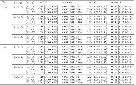
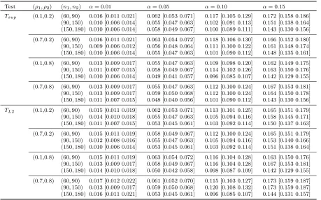
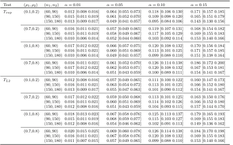
Table 3.2 Empirical type I error rates of the Tsup and TL2 tests based on Nsim = 3000
simulations and B = 500 bootstrap samples when mi = 30. The associated ±2 standard error are given in parentheses . . . 49 Table 3.3 Empirical type I error rates of the Tsup and TL2 tests based on Nsim = 3000
simulations and B = 500 bootstrap samples when mi ∼ {16, . . . ,20}. The
associated ±2 standard error are given in parentheses. . . 50 Table 3.4 Empirical type I error rates of the Tsup and TL2 tests based on Nsim = 3000
simulations andB = 500 bootstrap samples when mi ∼ {5, . . . ,9}. The
asso-ciated±2 standard error are given in parentheses. . . 51
Table 4.1 Empirical type I error rates for sparse sampling design based on 3000 simula-tions and 400 bootstrap samples. The associated ±2 standard error are given in parentheses. . . 69 Table 4.2 Observed values of test statistics and p-values of TL2, T2,L2 and T2,sup for
testing equality of the mean functions for the cat activity data. . . 73
Table A.1 Type I error rates of the GF based on true covariance in 3000 longitudinal data simulations with the tuning parameter δ and Case NP. The associated
±2 standard errors are given in parentheses. . . 98 Table A.2 Type I error rates of the pGF based on estimated covariance in 3000
longi-tudinal data simulations with the tuning parameter δ and Case EXP. The associated ±2 standard errors are given in parentheses. . . 99 Table A.3 Type I error rates of the GF based on true covariance in 3000 longitudinal
data simulations with the tuning parameterδ and Case EXP. The associated
±2 standard errors are given in parentheses. . . 99 Table A.4 Average computational time (in minutes) based on 5 simulations when n= 60 99 Table A.5 Type I error rates of the pGF based on estimated covariance in 3000
longi-tudinal data simulations with the tuning parameter δ = 2 and Case NP. The associated ±2 standard errors are given in parentheses. . . 101 Table A.6 Type I error rates of the pGF based on estimated covariance in 3000
Table A.7 Type I error rates of the pGFopt, pGF1, L2P and L2 based on 3000 longitudinal
functional data simulations for Cases [A1] NP and [B2] σ2
e,1 =σ2e,2 = 0. The
associated ±2 standard errors are given in parentheses. . . 107 Table A.8 Type I error rates of the pGFopt, pGF1, L2P and L2 based on 3000 longitudinal
functional data simulations for Cases [A2] EXP and [B1]σe,21 = 1.5 andσe,22 = 1. The associated ±2 standard errors are given in parentheses. . . 107 Table A.9 Type I error rates of the pGFopt, pGF1, L2P and L2 based on 3000 longitudinal
functional data simulations for Cases [A2] EXP and [B2] σ2e,1 =σ2e,2 = 0. The associated ±2 standard errors are given in parentheses. . . 107 Table A.10 Type I error rates of the pGFopt and pGF1 based on 3000 longitudinal
func-tional data simulations for Cases [A1] NP, [B1] σe,21 = 1.5 and σe,22 = 1 and [B2]σ2e,1 =σe,22 = 0. The associated±2 standard errors are given in parentheses.110 Table A.11 Type I error rates of the pGF1based on 3000 longitudinal functional data
sim-ulations with dimensionsK(n), Cases [A1] NP and [A2] EXP. The associated
±2 standard errors are given in parentheses. . . 111 Table A.12 Type I error rates of the pGF, GF and L2P based on 3000 longitudinal
func-tional data simulations for Cases [A1] NP and [B1] σe,21 = 1.5 and σe,22 = 1. The associated±2 standard errors are given in parentheses. . . 113 Table A.13 Type I error rates of the pGF1, pGF2, pGF4 and pGF8 based on 3000
lon-gitudinal functional data simulations for Cases [A1] NP, [B1] σe,21 = 1.5 and σe,22 = 1, and sample size n = 100. The associated ±2 standard errors are given in parentheses. . . 113
LIST OF FIGURES
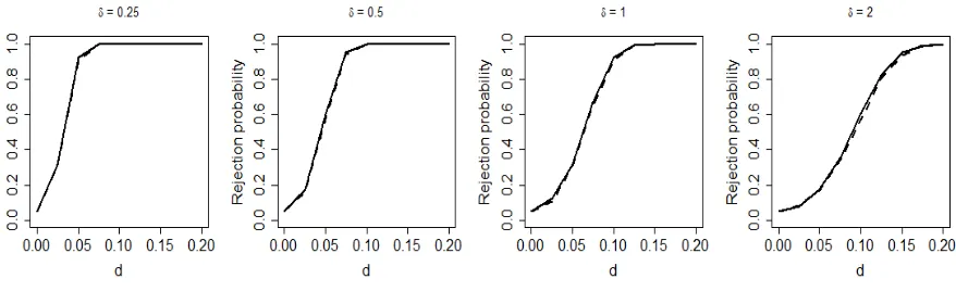
Figure 2.1 Power of the pGF based on estimated covariance (solid line) and the GF based on true covariance (dashed line) for δ,n= 300 and Case NP. Results are based on 1000 longitudinal data simulations and for a nominal level of 0.05. 25 Figure 2.2 Power of the pGFopt (solid line), pGF1 (dashed line), L2P (dotted line), L2
(dash-dotted line) for Cases [A1] NP and [B1] σ2
e,1 = 1.5 and σe,22 = 1 with
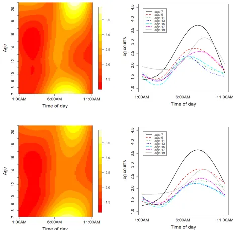
n = 100 (left panel) and n = 300 (right panel). Results are based on 1000 longitudinal functional data simulations and for a nominal level of 0.05. . . . 33 Figure 2.3 Image plots of estimated overall mean log counts as a bivariate function of
time of day and age for weekdays (top left panel) and for weekends (bottom left panel). Estimated overall mean log counts for seven different age groups for weekdays (top right panel) and for weekends (bottom right panel). . . 34 Figure 2.4 Powers of the pGFopt (solid line) and pGF1 (dashed line). Results are based
on 1000 simulations and for a nominal level of 0.05. . . 35
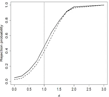
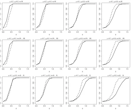
Figure 3.1 Empirical power curves of the Tsup (solid line) and TL2 (dashed line) tests
are displayed for sample sizes (n1, n2) = (90,150), g(s, t) = sin(3(s+ 1)2) +
exp(−5t2), andδ= 0, 0.2, 0.4, 0.6, 0.8, 1, 1.2, 1.4 and 1.6. Results are based on Nsim = 1000 simulations, B = 500 bootstrap samples, and a significance
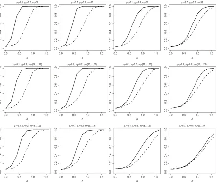
level α= 0.05. . . 53 Figure 3.2 Empirical power curves of the Tsup (solid line) and TL2 (dashed line) tests
are displayed for sample sizes (n1, n2) = (90,150), g(s, t) = 2.1t2s2, and δ =
0, 0.2, 0.4, 0.6, 0.8, 1, 1.2, 1.4 and 1.6. Results are based on Nsim = 1000
simulations, B = 500 bootstrap samples, and a significance level α= 0.05. . . 54 Figure 3.3 Estimated bivariate coefficient function αbd(s, t) corresponding to times
dur-ing 1:00 AM - 11:00 AM and day t in placebo group (left) and in treatment group (middle). The difference between estimates (right). . . 57 Figure 3.4 The null distributions of the Tsup test (left panel) andTL2 test (right panel)
based onB = 10000 bootstrap samples. The red dashed line is the 95 percent quantile of the null distributions of the Tsup and TL2 tests respectively. . . 58
Figure 4.1 Empirical power curves of the TL2 (solid line),T2,L2 (dashed line) andT2,sup
(dotted line) tests at the significance levelα= 0.05 forδ= 0, 0.5, 1.0, 1.5, 2.0, 2.5 and 3.0. Results are based on 1000 simulations and B = 400 bootstrap samples. The left panel and middle panel corresponds to the moderate sparse sampling design with sample sizes (n1, n2) = (20,30) and (n1, n2) = (40,60)
respectively. The right panel corresponds to the extreme sparse sampling design with sample size (n1, n2) = (40,60). . . 70
Figure 4.2 Estimated mean function µbd(s, t) corresponding to time s during 1:00 AM
Figure A.1 Powers of the pGF based on estimated covariance (solid line) and the GF based on true covariance (dashed line) forδ,n= 100 and Case EXP. Results are based on 1000 longitudinal data simulations and for a nominal level of 0.05. 99 Figure A.2 Powers of the pGF based on estimated covariance (solid line) and the GF
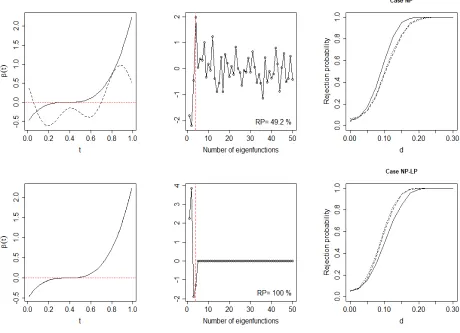
based on true covariance (dashed line) forδ,n= 300 and Case EXP. Results are based on 1000 longitudinal data simulations and for a nominal level of 0.05.100 Figure A.3 From top to bottom, panels are for Case NP and Case NP-LP respectively.
Left panels: departure from the null for Case (a) when d= 0.15, β(·) (solid line) and its approximation by the first 4 eigenfunctions (dashed line). Middle panels: hβ, uki corresponding to eigenfunctions and RP. Right panels: powers
of the pGF for mi ∼ {7, . . . ,12} (solid line), mi ∼ {22, . . . ,28} (dashed
line) and mi ∼ {42, . . . ,48} (dotted line), based on 1000 longitudinal data
simulations and for a nominal level of 0.05. . . 103 Figure A.4 From top to bottom, panels are for Case NP and Case NP-LP respectively.
Left panels: departure from the null for Case (b) when d= 0.15, β(·) (solid line) and its approximation by the first 4 eigenfunctions (dashed line). Middle panels: hβ, uki corresponding to eigenfunctions and RP. Right panels: powers
of the pGF for mi ∼ {7, . . . ,12} (solid line), mi ∼ {22, . . . ,28} (dashed
line) and mi ∼ {42, . . . ,48} (dotted line), based on 1000 longitudinal data
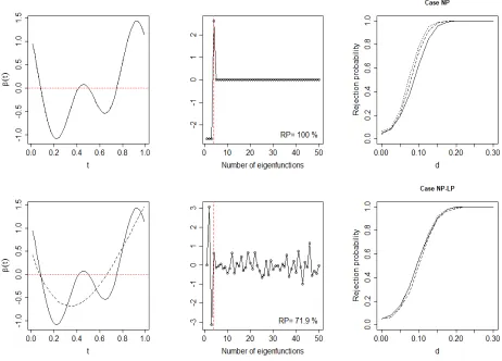
simulations and for a nominal level of 0.05. . . 104 Figure A.5 From top to bottom, panels are for Case NP and Case NP-LP respectively.
Left panels: departure from the null for Case (c) when d= 0.15, β(·) (solid line) and its approximation by the first 4 eigenfunctions (dashed line). Middle panels: hβ, uki corresponding to eigenfunctions and RP. Right panels: powers
of the pGF for mi ∼ {7, . . . ,12} (solid line), mi ∼ {22, . . . ,28} (dashed
line) and mi ∼ {42, . . . ,48} (dotted line), based on 1000 longitudinal data
simulations and for a nominal level of 0.05. . . 105 Figure A.6 Orthonormal cubic B-spline basis functionφk(s),k= 1,2. . . 106
Figure A.7 Power of the pGFopt (solid line), pGF1 (dashed line), L2P (dotted line), L2
(dash-dotted line) for Cases [A1] NP and [B2] σ2
e,1 =σ2e,2 = 0 with n = 100
(left panel) andn= 300 (right panel). Results are based on 1000 longitudinal functional data simulations and for a nominal level of 0.05. . . 108 Figure A.8 Power of the pGFopt (solid line), pGF1 (dashed line), L2P (dotted line), L2
(dash-dotted line) for Cases [A2] EXP and [B1] σe,21 = 1.5 and σe,22 = 1 with n = 100 (left panel) and n = 300 (right panel). Results are based on 1000 longitudinal functional data simulations and for a nominal level of 0.05. . . . 108 Figure A.9 Power of the pGFopt (solid line), pGF1 (dashed line), L2P (dotted line), L2
(dash-dotted line) for Cases [A2] EXP and [B2] σe,21=σe,22= 0 withn= 100 (left panel) andn= 300 (right panel). Results are based on 1000 longitudinal functional data simulations and for a nominal level of 0.05. . . 109 Figure A.10 Powers of the pGF1for Case [A1] NP (top panels) and Case [A2] EXP (bottom
Figure A.11 Powers of the pGF (solid line), GF (dashed line) and L2P (dotted line) for Cases [A1] NP and [B1]σ2
e,1= 1.5 andσe,22= 1 with sample sizen= 100 (left
panel) and n = 300 (middle panel). Right panel: powers of the pGF (solid line), pGF1 (red dashed line), pGF2 (red dotted line), pGF4 (blue dashed line), pGF8 (blue dotted line), GF (dashed line) and L2P (dotted line) for sample size n= 100. Results are based on 1000 longitudinal functional data simulations and for a nominal level of 0.05. . . 114 Figure A.12 Average of activity profiles for 58 cats across days are shown in gray for
weekdays (left panel) and weekends (right panel) respectively. Overall mean profiles for weekdays and weekends are shown in blue and red respectively. Horizontal dashed lines indicate the time window 1:00 AM - 11:00 AM. . . . 116 Figure A.13 Left panels: the estimated time-varying effect of DJD score,β(s, t), over daysb
t and time of days during 1:00 AM - 11:00 AM (top) and its average across dayst(bottom). Right panels: the estimated time-varying effect of DJD score,
b
β(s, t), over days t and 24 hours a days (top) and its average across days t (bottom). The dashed line indicates the time window 1:00 AM - 11:00 AM. . 117 Figure A.14 Activity profiles during 1:00 AM - 11:00 AM from two different cats (left
col-umn) and average of log counts (right colcol-umn) are displayed. The horizontal axis on the right panels indicates repeated time (day) and day of the week that cat was observed. The average on the time window is connected with all cat’s observation day. Red square point and blue triangle point on the right column correspond to activity profiles highlighted as red solid line and blue dotted line on left column respectively. . . 118 Figure A.15 The estimated time-varying effect of DJD scoreβ(t), over daysb t. . . 119
Figure A.16 The estimated optimal projection functionφbopt. . . 119
Figure A.17 Left panel:β(b ·) (solid line) and a linear combination of first 2 leading
eigen-functions of estimated covariance (dashed line). Right panel: hβ,b buki
corre-sponding to eigenfunctions of estimated covariance, ubk(·) for k= 1, . . . ,20. . . 120
Figure A.18 Original data of randomly selected cat (left panel) and one simulated data (right panel when d = 1. For illustration two activity profiles are randomly highlighted as red solid line and blue dotted line respectively. . . 122 Figure A.19 Average of original log counts for each subject (left panel) and corresponding
avereage of simulated one (right panel) when d= 1. For illustration observed average of log counts from two randomly selected cats are highlighted as red solid line and blue dotted line respectively. . . 122
Figure B.1 Functiong(s, t) =sin(3(s+ 1)2) +exp(−5t2) (left panel) andg(s, t) = 2.1t2s2
(right panel) are displayed. . . 126 Figure B.2 Empirical power curves of the Tsup (solid line) and TL2 (dashed line) tests
for sample sizes (n1, n2) = (60,90), g(s, t) =sin(3(s+ 1)2) +exp(−5t2), and
δ = 0, 0.2, 0.4, 0.6, 0.8, 1, 1.2, 1.4 and 1.6. Results are based onNsim= 1000
Figure B.3 Empirical power curves of theTsup(solid line) andTL2 (dashed line) tests for
sample sizes (n1, n2) = (60,90),g(s, t) = 2.1t2s2, andδ= 0, 0.2, 0.4, 0.6, 0.8,
1, 1.2, 1.4 and 1.6. Results are based on Nsim = 1000 simulations, B = 500
bootstrap samples, and a significance level α= 0.05. . . 128 Figure B.4 Empirical power curves of theTsup(solid line) andTL2 (dashed line) tests for
sample sizes (n1, n2) = (150,180), g(s, t) =sin(3(s+ 1)2) +exp(−5t2), and
δ = 0, 0.2, 0.4, 0.6, 0.8, 1, 1.2, 1.4 and 1.6. Results are based onNsim= 1000
simulations, B = 500 bootstrap samples, and a significance level α= 0.05. . . 129 Figure B.5 Empirical power curves of the Tsup (solid line) and TL2 (dashed line) tests
for sample sizes (n1, n2) = (150,180), g(s, t) = 2.1t2s2, and δ = 0, 0.2, 0.4,
0.6, 0.8, 1, 1.2, 1.4 and 1.6. Results are based on Nsim = 1000 simulations,
B = 500 bootstrap samples, and a significance level α= 0.05. . . 130
Chapter 1
Introduction
1.1
Overview
Functional Data Analysis (FDA) is a modern statistical method which is widely implemented to
deal with analysis and theory of data that are in form of function, surfaces and high-dimensional
objects. In FDA, observed data are considered to be sample of function defined on some continuous
domain and to be sampled in a discrete fashion; each sample is usually observed at finite grid points.
Rapid development of modern computation and technology facilitates to collect such massive data
that have high intrinsic dimensionality so that FDA becomes commonly used statistical techniques
and has been studied extensively. For comprehensive review of FDA, we refer to monographs; e.g.
Ramsay & Silverman (2005); Ferraty & Vieu (2006); Ramsay et al. (2009); and Horv´ath & Kokoszka
(2012) among others.
In the real world, the functional data are commonly recorded in the finite discrete values,
often with noise. Suppose that we have the observed functional data, {(si`, Yi`) :i= 1, . . . , n;`=
1, . . . , Li}, where Yi` is the `th repeated measurement for the ith subject observed at the time
point si` ∈ S for a compact set S. In FDA, the observed values {Yi` :`= 1, . . . , Li} are assumed
to be an independent realization of an underlying stochastic process on a finite grid of design time
the observed data Yi` are modeled as
Yi`=Xi(si`) +εi`, (1.1)
whereXi(·) are independent and identically distributed (iid) random samples of a square integrable
latent processX(·) inL2(S) with unknown smooth mean and covariance function, and measurement errors εi` are iid random errors with zero-mean and finite variance.
Although many theories and methodologies for FDA have been established in the underlying
process, in practice the process is latent, and the data only can be collected on regular or irregular
discrete gird points. Further the number of discrete points can vary over subjects. In general, FDA
considers two types of sampling designs: (i) dense sampling design where the set of time grid for
each subject, {si` :` = 1, . . . , Li}, is dense in S and (ii) sparse sampling design where the set of
sampling points for each subject,{si`:`= 1, . . . , Li}, is random and irregular, further the number
of measurement for each subject, Li, is quite small. See Zhang et al. (2016) for general review.
Although there have been rich development for theoretical and application in FDA, most
ex-isting methodologies focus on the case where each subject has a single curve, which allows the
independent sample of functions as described in (1.1). Recently, correlated functional data where
multiple functions are observed from the same subject or unit have been increasingly investigated in
many scientific fields and have received much attention. Such functional data have strong
between-function correlation induced by the experimental design where multiple between-functions are observed
repeatedly over time for each of subjects. Therefore, existing methodologies that assumed the
in-dependent sample of functions cannot account for the complex correlated structure that consists
of between-function correlation and within-function correlation, which inspires development of new
methodologies for such correlated functional data.
There have been existing studies for the correlated functional data structure, for example,
in-cluding multilevel (Morris & Carroll (2006); Crainiceanu et al. (2009); Di et al. (2009); Di et al.
Staicu (2015); Scheipl et al. (2015); Chen et al. (2017)), and spatially correlated
(Baladandayutha-pani et al. (2008); Staicu et al. (2010); Staicu et al. (2015)). Although there are some growing
literature that account for complex correlation induced by multilevel and longitudinal design, more
development is still needed to capture these sources of variability efficiently and accurately.
In this thesis, we focus on longitudinally observed functional data, commonly referred as
longi-tudinal functional data, where functions, e.g. profiles or images, are observed sequentially over time
or repeated instances (often, times of visit) from each of many subjects. An example of
longitudi-nal functiolongitudi-nal data application as well as motivated our work is a longitudilongitudi-nal study of cat with
osteoarthritis (Gruen et al. (2015); Gruen et al. (2017b)). For each of 58 indoor cats who suffer
from osteoarthritis, we have daily physical activity profiles measured at 1 minute epoch level over
multiple days.
Our main scientific questions in this thesis involve: (i) to formally assess the association between
daily physical activity profiles and scalar covariates such as disease severity score, age and day of
week (weekend or weekday) (ii) to examine whether the covariate effect on daily physical activity
profiles differ between placebo and treatment groups over time and (iii) to formally assess difference
among multiple group mean profiles. Although these types of questions are very common in the
context of function-on-scalar regression, most developed methodologies are intended for independent
samples of functions and there are very limited inferential methods that account for
between-function correlation and within-between-function correlation induced by longitudinal design. We develop
practically applicable testing procedures that are designed for complex correlated functional data,
where densely or sparsely sampled in longitudinal design, and with measurement errors.
Main research direction in this thesis is to formally assess the association between functional
responses and scalar covariate/s using functional regression techniques. There have been rich
lit-erature for functional regression models. Functional regression model generally can be classified
into three types depending on whether one or both of response and covariates have functional or
scalar characteristics: (i) scalar-on-function regression model with scalar responses and functional
and (iii) function-on-scalar regression model (or functional response regression model) with
func-tional responses and scalar predictors. Function-on-scalar regression is a relevant area that has been
studied to assess the relationship between functional responses and scalar covariate/s. For example,
functional analysis of variance (FANOVA) model (Staniswalis & Lee (1998); Spitzner et al. (2003);
Abramovich & Angelini (2006); Zhang et al. (2013); Zhang (2013); Zhang & Liang (2014); Smaga &
Zhang (2018)), regression for independent functional responses (Chiou et al. (2004); Ferraty & Vieu
(2006); Reiss et al. (2010)), and regression for correlated functional responses (Morris & Carroll
(2006); Scheipl et al. (2015); Goldsmith et al. (2015); Goldsmith & Kitago (2016)). For
comprehen-sive review for functional regression, see Morris (2015). In this thesis we consider function-on-scalar
regression for function data where data framework consists of (i) multiple functional samples
ob-served at repeated measures (e.g. days or times of visit) for the same subject and (ii) multiple scalar
covariates including group factor, subject level covariates and longitudinally repeated measures.
1.2
Contributions and outline
This thesis consists of three projects that are motivated by the longitudinal study of cat with
osteoarthritis. The cat activity study is a crossover, randomized, double masked and placebo
con-trolled clinical trial. Total of 58 client-owned cat with osteoarthritis were randomly divided into
two groups and each group received placebo and active treatment during four specific periods: (i)
baseline period, (ii) the first treatment period, (iii) wash-out period and (iv) the second treatment
period. Each period has around 20 days except for baseline period (13 days). To be specific cats in
the first group received active treatment during the first treatment period and placebo during the
second treatment period, while cats in the second group had reverse order; they received placebo
first and active treatment later during two treatment periods. All cats took placebo during
base-line and wash-out periods. Further placebo and active treatment were masked to avoid recognition
to cat owners and investigators. Throughout all periods, cat’s physical activity were measured at
1 minute epoch level by an activity monitor attached on each cat’s neck collar. Specifically each
measurements. This study also includes other information such as baseline disease severity scores
(DJD score and pain score), day of week (Monday - Sunday) and age. Our works in this thesis
strongly connected to this longitudinal functional data and related scientific questions.
In chapter 2 we develop inferential approaches to study the association between one-dimensional
functional response and scalar covariates observed in longitudinal design over repeated instances.
A primary objective of this study is to formally assess daily-varying effects of disease severity on
physical activity of cats. To address this problem, we develop a likelihood ratio-inspired testing
procedure. We consider a time-varying functional regression model framework to study covariate
effect varying over longitudinal time (e.g. days) domain but not varying over functional time (e.g.
time of a day) domain. This time-invariant effect of covariate in functional time domain allows us to
project the model components onto the functional direction and obtain the projection-based reduced
model framework. The projection function plays an important role and we propose an optimal
projection function that minimizes magnitude of random deviations. Then we obtain a mixed effects
model framework by using mixed effects model representation of fixed effects and reformulate the
hypotheses of interest to testing that fixed effect parameters and a variance component are zero.
This is a common testing problem in context of mixed effects model, but the mixed effects model
involves unknown, complex error dependence structure induced by between-function correlation
and multiple variance components. To solve this problem we propose a novel method based on a
low-rank approximation to de-noise dependent data to conduct the proposed test efficiently. Further
theoretical properties are studied, and numerical investigations confirm excellent performance of
proposed test in terms of size and power in various scenarios. The proposed test procedure is
illustrated on the data application.
In chapter 3 we propose inferential methods for complex correlated functional data about
group-specific covariate effects in two groups. The method is inspired by the cat activity data where it is
expected that active treatment alleviates osteoarthritis-associated pain and improves cat’s activity.
Our primary objective is to investigate whether baseline pain score effects are different over time
of functions is observed at fine grid points. The group-specific covariate effects are captured by the
bivariate coefficient functions on longitudinal and functional time domain. We propose L2-norm and supremum-norm based test statistics, further develop two-step estimation method to estimate
bivariate functions. Two-step estimation method consists of (i) the least square estimation and
(ii) smoothing step, which is computationally fast and feasible for even large sample sizes. We
consider permutation-based bootstrap of independent unit (e.g. subject) to approximate the null
distributions of the test statistics. Extensive simulations exhibit excellent numerical performance
of proposed tests in terms of size controlling and power, and methods are applied to the motivating
data example.
In chapter 4 we shift our focus to testing about equality of multiple group mean functions in
longitudinal functional data. We consider a functional response model for longitudinal functional
data in flexible data structure: (i) functional samples are observed at regular or irregular grids
with measurement errors and (ii) more than two samples of curves are observed. Therefore this
work extends the previous study by relaxing the assumptions that curves are observed on
regu-lar grid points in two groups. We propose an L2-norm based testing procedure for testing group
mean differences. We estimate two-dimensional group mean functions under a working
indepen-dence assumption by using bivariate smoothing approaches for sparse functional data and then
use bootstrap over independent unit (e.g. subject) that accounts for the complex data dependence.
Simulations show excellent numerical performance in terms of size for the proposed test in small
sample sizes or extreme sparse sampling design. Methods developed in this chapter also applied to
cat activity study as illustrative example. In this chapter we investigate whether there is difference
Chapter 2
Significance test for time-varying
covariate effect in longitudinal
functional data
2.1
Introduction
We study statistical inference for regression model involving one-dimensional curve responses that
are observed repeatedly, over multiple times of visit per subject, for many subjects. This form of
correlated functional data is often referred to aslongitudinal functional data (Greven et al. (2010);
Chen & M¨uller (2012); Park & Staicu (2015)). For example, in our motivating application,
minute-by-minute daily activity profiles are measured repeatedly over several days for many cats with
osteoarthritis and the goal is to formally assess whether the cat’s physical activity is related to
their disease severity. We study this problem by assuming that, during a time window 1:00 AM
-11:00 AM, disease severity effect varies across days but is invariant within the time window.
Modeling correlated functional data has received a lot of attention in the literature. Morris &
Carroll (2006) introduced a Bayesian wavelet-based functional mixed effects model. Di et al. (2009)
et al. (2014) extended the methodology to handle sparsely observed functional data. Staicu et al.
(2010) proposed a functional response model for spatially correlated multilevel functional data.
Greven et al. (2010) considered a longitudinal functional model with functional random intercept
and slope. Models for longitudinal functional responses have been also proposed by Chen & M¨uller
(2012); Park & Staicu (2015); Chen et al. (2017). Function-on-scalar regression models, when both
the responses and the covariates are observed in longitudinal design, have been discussed by Scheipl
et al. (2015) for continuous valued responses and by Goldsmith et al. (2015) for binary valued
responses.
Although these studies mainly focus on modeling, there is limited literature on statistical
in-ference involving this type of data. For example, inin-ference about the difin-ference of mean functions
between two correlated functional samples has been studied by Crainiceanu et al. (2012) through
bootstrap-based inferential methods and by Staicu et al. (2014) through a pseudo likelihood
ratio-based testing approach. Significance test for the equality of multiple group mean functions in
correlated functional data has been also considered by Staicu et al. (2015) using anL2-norm-based testing procedure. Inference for covariate effect has been considered recently by Park et al. (2017)
who proposed an L2-norm-based test. While this paper is the closest to our problem of interest, it involves nonparametric bootstrap-based inferential methods that are computationally intensive
and further it has lower power in detecting true signal.
In this paper, we consider a time-varying functional regression for longitudinal functional
re-sponses and scalar covariates. We study significance test of time-varying covariate effect on the
responses and develop a likelihood ratio-inspired testing procedure. We assume that observations
within each curve response are observed on fine grids (i.e. dense functional design), but curve
re-sponses for each subject are observed in sparse sampling design (i.e. sparse longitudinal design).
Furthermore, we assume that the covariate of interest is time-invariant and the covariate effect does
not change over functional arguments but change over longitudinal arguments. This assumption
allows us to project model components onto a direction of functional space and obtain a
(2002). Inference in functional mixed effects models has been considered; for example, Guo (2002)
proposed a likelihood ratio test (LRT) and its asymptotic null distribution derived by Self & Liang
(1987), however, that requires heavy computational cost and restrictive conditions to apply the
asymptotic theory (see Crainiceanu & Ruppert (2004)); Antoniadis & Sapatinas (2007) and Zhang
& Chen (2007) proposed an F-based test and anL2-norm-based test, however, developed for dense sampling design, while we focus on the sparse sampling design.
Our testing approach is mainly based on mixed effects model representations of fixed
(population-level) effects (Ruppert et al. (2003)). A mixed effects model framework corresponding to our
projection-based reduced model incorporates correlated errors induced by multiple observations
across times of visit on the same subject. The initial null hypothesis is reformulated as testing
that fixed effect parameters and a variance component are zero in a mixed effects model that
con-tains additional variance components and general error covariance structure. Developing a testing
method based on a mixed effects model representation is one of common approaches. For example,
Wang & Chen (2012) derived a generalized F test and its finite sample null distribution for a mixed
effects model with multiple variance components but independent and identically distributed (i.i.d.)
errors. Staicu et al. (2014) derived a pseudo likelihood ratio test and its asymptotic null distribution
in a mixed effects model with unknown, general error covariance structure but a single variance
component.
We consider a pseudo generalized F test that can be viewed as an extension of testings of Wang
& Chen (2012) and Staicu et al. (2014). Our testing is applicable to unknown, non-trivial error
covariance structure induced by longitudinal dependence in our context, and multiple variance
components. The main contributions of this paper are to propose (i) the new and fast testing
procedure for the time-varying covariate effect on longitudinal functional responses with complex
correlated structures; (ii) optimal choice of the projection function that minimizes magnitude of
random deviation; and (iii) a new method for de-noising dependent data based on a low-rank
approximation of covariance to conduct the pseudo generalized F test efficiently. Furthermore, the
This paper is organized as follows. Section 2.2.1 introduces longitudinal functional data
struc-ture, modeling framework and hypothesis. We propose the projection-based reduced model and the
mixed effects model representation in Section 2.2.2. Section 2.3 proposes the pseudo generalized F
test. We introduce the method to de-noise dependent data in Section 2.3.1 and optimal selection of
the projection function in Section 2.3.2. Section 2.4 describes estimation methods and
implementa-tion. Section 2.5 provides some theoretical properties for the pseudo generalized F test. Simulation
results and motivating data application are presented in Section 2.6 and Section 2.7 respectively.
Section 2.8 contains a brief discussion.
2.2
Data structure and models
2.2.1 Model framework and problem definition
The observed data for theith subject is [{Yij(s), tij :s∈ S}mj=1i , Wi], whereYij(·) is one-dimensional
curve observed at the jth time of visit since the baseline, tij, for j = 1, . . . , mi, and Wi is a
baseline covariate of interest of the ith subject. In practice, the curves Yij(·) are observed at a
finite grid{sij1, . . . , sijLij}; measurements are collected as (Yij`, sij`) for`= 1, . . . , Lij. We assume
a sparse sampling design for the longitudinal argument tij: the number of repeated measurements
per subject,mi, is small and {tij :j= 1, . . . , mi} is sparse, but{tij :i= 1, . . . , n;j= 1, . . . , mi} is
dense in a closed and bounded set T. We also assume a dense sampling design for the functional
arguments:{sij` :`= 1, . . . , Lij}is dense in a closed and bounded setS. Without loss of generality,
assume thatsij` =s` forms an equally spaced grid of points in S and use the indexsinstead ofs`.
Our main interest is to formally assess the association between the covariate of interest, Wi,
and the functional responses Yij(·). For example, in our motivating data, Yij(s) corresponds to
the physical activity of the ith cat on the jth day at time s varying from 1:00 AM to 11:00 AM,
and Wi is the cat’s baseline disease severity score. We study this problem under the assumption
that the covariate effect varies with the longitudinal argumenttbut is constant over the functional
the disease severity and activity does not change during the pre-specified time window but can vary
across days. To this end, we posit a functional regression model
Yij(s) =µ(s, tij) +Wiβ(tij) +εi(s, tij), (2.1)
whereµ(·,·) is an unknown smooth intercept function defined onS × T,β(·) is an unknown smooth
coefficient function defined onT, andεi(·, tij) is a zero-mean random deviation defined onS. Scheipl
et al. (2015); Goldsmith et al. (2015); Park et al. (2017) have discussed estimation of various model
parameters and response prediction under this model framework. Our goal is to test the hypothesis
of no covariate effect, that is test the hypothesis
H0 :β(·) = 0 versusHa:β(·)6= 0. (2.2)
A possible testing approach for this hypothesis is anL2-norm-based testing procedure suggested by
Park et al. (2017) that used bootstrap-based methods to approximate its null distribution. However,
its nonparametric bootstrap-based methods require high computational cost. In this paper, we
propose a computationally fast and feasible testing method for assessing the significance of β(·).
The methodology can easily accommodate additional covariates through additive effects.
2.2.2 Projection-based reduced model
We propose a testing procedure that relies on the fact that the covariate effectβ(·) is invariant to
the functional argument s. Let φ(·) be a function in L2(S) such that R
Sφ(s)ds6= 0 and consider
the projection of model (2.1) onto φ(·). We discuss the choice of φ(·) in Section 2.3.2. Define
Yφ,ij =
R
SYij(s)φ(s)ds as the projected response and similarly define µφ(tij) =
R
Sµ(s, tij)φ(s)ds
and aφ=
R
Sφ(s)ds. The projected model implied by (2.1) is
where εφ,i(tij) is a random deviation of the projected response from the subject-specific trend
corresponding to directionφ. We study the hypothesis testing problem (2.2) in model (2.3).
The model (2.3) is a functional mixed effects model and inference in this model framework has
been previously studied. Guo (2002) modeled smooth effects by using smoothing splines for testing
(2.2) and proposed a LRT. However, Guo (2002) used the asymptotic null distribution developed
by Self & Liang (1987), which has restrictions pointed out by Crainiceanu & Ruppert (2004). The
inferential methods are computationally intensive and scale poorly with increasing sample size.
For the same testing problem, Antoniadis & Sapatinas (2007) modeled the smooth effects using
wavelet basis and proposed an F-based testing procedure, which however requires that the number
of measurements per curve is constant across subjects and further is a power of 2. Zhang & Chen
(2007) also considered the dense sampling design and developed an L2-norm-based test and its asymptotic null distribution. In contrast we focus on the sparse sampling design for tij’s.
We model the smooth population level effects µφ(·) and β(·) by using truncated polynomial
basis: µφ(t) = µφ,0 +µφ,1t+. . .+µφ,p1t
p1 +Ph1
h=1bφ,1h(t−τ1h) p1
+ and β(t) = β0 +β1t+. . .+
βp2t
p2 +Ph2
h=1b2h(t−τ2h) p2
+, where τ1h and τ2h are knots and (x)p+=xp ifx >0 and 0 otherwise.
The knots are chosen based on equally spaced sample quantiles and the numbers of knots, h1
and h2, are taken to be sufficiently large for flexibility; see Ruppert et al. (2003) and Ruppert
(2012). In matrix notation, we have µφ(tij) = CT1,ijβ φ
1 +ZT1,ijb φ
1 and β(tij) = CT2,ijβ2+ZT2,ijb2,
where C1,ij = (1, tij, . . . , tpij1)T,C2,ij = (1, tij, . . . , tpij2)T,Z1,ij ={(tij −τ11)+p1, . . . ,(tij −τ1h1)
p1
+}T, Z2,ij = {(tij −τ21)+p2, . . . ,(tij − τ2h2)
p2
+}T, β φ
1 = (µφ,0, . . . , µφ,p1)
T, β
2 = (β0, . . . , βp2)
T, bφ 1 =
(bφ,11, . . . , bφ,1h1)
T andb2= (b
21, . . . , b2h2)
T. As it is common in these settings, we treatβφ
1 and β2
as unknown but fixed parameters and bothbφ1 andb2as random parameters withbφ1 ∼N(0, σ2b1Ih1)
and b2 ∼ N(0, σ2b2Ih2). Here N(0,B) denotes the multivariate normal distribution with mean 0
and covarianceB, and Ig denotes theg×g identity matrix.
Let Yφi = (Yφ,i1, . . . , Yφ,imi)
T,εφ
i = (εφ,i(tij), . . . , εφ,i(timi))
T,C
1i a mi×(p1+ 1) matrix with
thejth row C1,ij,C2i a mi×(p2+ 1) matrix with thejth rowC2,ij,Z1i ami×h1 matrix with the
associated to (2.3) is given by
Yiφ=C1iβφ1 +aφWiC2iβ2+Z1ibφ1 +aφWiZ2ib2+εφi, i= 1, . . . , n, bφ1 ∼N(0, σb2
1Ih1),
b2∼N(0, σ2b
2Ih2),
εφi ∼N(0,Σi), and
bφ1,b2 and εφi are independent,
(2.4)
whereΣi is a mi×mi unknown covariance matrix. In fact, the covariance matrix Σi is Σi =Σφ,i
because it depends on the projection functionφ. For convenience, we suppress the subscript φ. In
this model, hypotheses (2.2) are reformulated as
H0:β2=0and σ2b2 = 0 versusHa:β2 6=0 orσ
2
b2 >0. (2.5)
Research on hypothesis testing for both fixed effect parameters and a variance component as
in (2.5) in mixed effects models has been prompted by Crainiceanu & Ruppert (2004) who studied
the problem for a single variance component model with independent errors, i.e. Σi =σ2Imi and
derived finite sample and asymptotic distributions of the LRT. Wang & Chen (2012) proposed
a generalized F test for multiple variance components model with independent errors. However,
as expected, both lead to inflated Type I error rates when applied directly to models involving
correlated data. On the other hand, Staicu et al. (2014) assumed complex, unknown error covariance
structure and used an inverse square root of Σi, denoted by Σ−1i /2, to de-noise dependent errors
and then proposed a pseudo LRT, however, for a single variance component model. In the following
section, we propose (i) a new testing approach that can handle both multiple variance components
and complex error covariance structure and (ii) a new de-noising method based on a low-rank
approximation of covariance that gives computationally efficiency and better size performance of
2.3
Pseudo generalized F test
In this section, we describe the pseudo generalized F test to study (2.5). Denote the vector ofYiφ’s byYφ, the vector ofεφi’s byεφ, the stacked matrix ofC1i’s byC1, the stacked matrix ofaφWiC2i’s
byC2, the stacked matrix of Z1i’s byZ1, and the stacked matrix ofaφWiZ2i’s by Z2, respectively.
Let Σ be the block diagonal matrix of Σi’s andN = Pni=1mi be the length of Yφ. The stacked
model is given by Yφ=C1βφ1 +C2β2+Z1bφ1 +Z2b2+εφ.
If the covariance Σ was known, let Mi be a mi ×m˜i matrix such that MTi ΣiMi = σ2Im˜i
with ˜mi ≤ mi for i = 1, . . . , n. We discuss how to define the de-noising matrix Mi in Section
2.3.1. Denote by M the N ×N˜ block diagonal matrix of Mi’s, where ˜N = Pni=1m˜i. By
left-multiplying the stacked model by MT, we obtain a model MTYφ = MTC1βφ1 +MTC2β2 + MTZ1bφ1 +MTZ2b2+MTεφ. Now the generalized F test (GF in short) of Wang & Chen (2012)
can be used in this transformed model since the transformed error is MTεφ ∼ N(0, σ2IN˜). The
GF statistic consists of the residual sum of squares (RSS) under the null and alternative. RSS
under the null is RSS0M(γ) = (Yφ−C1βcφ1)TMV−10M(γ)MT(Yφ−C1βcφ1)/σ2, where V0M(γ) = IN˜ +γMTZ1Z1TM,γ =σ2b1/σ
2 and βcφ
1 ={CT1MV −1
0M(γ)MTC1}+CT1MV −1
0M(γ)MTYφ. HereA+
denotes the Moore-Penrose inverse of a matrix A. RSS under the alternative is RSS1M(γ, λ) =
(Yφ−Cβcφ)TMV−1
1M(γ, λ)MT(Yφ−Cβc
φ)/σ2, whereV
1M(γ, λ) =V0M(γ) +λMTZ2ZT2M,βcφ= {CTMV−1
1M(γ, λ)M
TC}+CTMV−1
1M(γ, λ)M
TYφ, λ=σ2 b2/σ
2 and C= [C
1,C2]. The GF statistic
is defined as GFN˜ = ˜N{RSS0M(bγ)−RSS1M(γ,b λ)b }/RSS1M(γ,b bλ), where bγ andλbare obtained by
the restricted maximum likelihood (REML) under the alternative model. The finite sample null
distribution of the GF statistic, derived by Wang & Chen (2012), is
GFN˜ = ˜d N
Ph2
s=1
b
λρs(bγ)
1+λρb s(bγ)
u2s+Pp2
s=1vs2
Ph2
s=1 1+bλρ1
s(bγ)
u2 s+
PN˜−p1−p2
s=h2+1 u
2 s
, (2.6)
whereu2si.i.d.∼ χ21 fors= 1, . . . ,N˜−p1−p2,v2s i.i.d.
∼ χ21 fors= 1, . . . , p2,ρs(γ) is thesth eigenvalue of ZT2M[V−10M(γ)−V−10M(γ)MTC{CTMV−1
0M(γ)MTC}+CTMV −1
0M(γ)]MTZ2, the notation d
equality in distribution, and bγ and bλare the values that maximize the spectral decomposition of
the restricted profile log-likelihood under the alternative model up to a constant,
f(γ, λ) =−( ˜N−p1−p2)log
h2 X s=1 1 1 +λρs(γ)
u2s+
˜ N−p1−p2
X
s=h2+1
u2s
− h2 X s=1
log{1+λρs(γ)}− h1
X
s=1
log(1+γωs),
whereωs is thesth eigenvalue of ZT1{MMT −MMTC(CTMMTC)+CTMMT}Z1.
In practice, however the covarianceΣand implicitlyMare unknown, and thus directly applying the GF is not feasible. However, if we had a consistent estimator of Σ, then we can construct a version ofMin the same way as above, and use the test with a corresponding plug-in estimator. Let
b
Σbe a consistent estimator of Σand Mc be a consistent estimator of M that satisfiesMcTΣbMc =
σ2IN˜. We propose the test statistic
pGFN˜ = ˜N
[ RSS0
c
M(bγ)−RSS[1Mc(bγ,
b
λ)
[ RSS1
c
M(γ,b bλ)
, (2.7)
whereRSS[0
c
M(γ) and RSS[1Mc(γ, λ) are readily obtained by substitutingMwith
c
MinRSS0M(γ)
and RSS1M(γ, λ) respectively. We call it pseudo GF (pGF in short) statistic to recognize that the
estimated error covariance was used, and not the true value.
Since the finite sample null distribution of the GF in (2.6) basically depends on the eigenvalues
ρs(γ)’s andωs’s, asymptotic null distributions of the GF and pGF may depend on the asymptotic
behavior of these eigenvalues. We assume that the eigenvaluesρs(γ) and ωs have their limits with
a proper convergence rate as n → ∞. Then the asymptotic null distribution of the GF with M
may consist of these limits of eigenvalues. Let ρbs(γ) and ωbs be defined similarly to ρs(γ) and ωs
by replacing M with Mc. The convergence of ρbs(γ) and ωbs to ρs(γ) and ωs respectively for every
sbased on the consistency of cMmay imply that the null distribution of the GF is asymptotically
equivalent to that of the pGF. We show the convergence of eigenvalues ρbs(γ) and ωbs under the
reasonable in all our numerical studies. However, it is hard to show that convergence of eigenvalues
always holds in the Moore-Penrose inverse as the general case. It is still intuitively reasonable to
use the finite sample null distribution (2.6) obtained by plugging inMc forMas an approximation
of the asymptotic null distribution of the pGF. The asymptotic null distribution of the pGF will be
well approximated in the large sample. Simulation studies also show that using this approximation
yields a good size and power performances. The estimation of Σ and M is described in Section 2.4.2, while the convergence of Mc is discussed in Section 2.5. For completeness we describe below
the algorithm to sample from the null distribution.
Step 1 Compute eigenvaluesρbs(γj) at a specified grid of points {γ1, . . . , γm}.
Step 2 Simulate ˜N −p1 −p2 independent χ21 random variables u2s and p2 independent χ21 random
variables v2s.
Step 3 Compute f(γj, λ`) with ωbs and pre-computed ρbs(γj) over grid of points {γ1, . . . , γm} and
{λ1, . . . , λm}, and determineγmax and λmax which maximizef(γj, λ`) over the grids.
Step 4 Compute the right-hand side in (2.6) by using λmax and ρbs(γmax).
Step 5 Repeat Steps 2 - 4.
2.3.1 Selection of the signal de-noising matrix Mi
We propose the de-noising matrix Mi based on a low-rank approximation. To begin with, let
εφ,i(tij) =
R
Sεi(s, tij)φ(s)dsbe i.i.d. stochastic process with zero-mean and assume their covariance
Σφ(t, t0) = cov{εφ,i(t), εφ,i(t0)}=
R R
Scov{εi(s, t), εi(s0, t0)}φ(s)φ(s0)dsds0<∞ for all t, t0 ∈ T. We
also assume that the covariance Σφ(t, t0) is Σφ(t, t0) = Γφ(t, t0) +σφ,e2 1(t=t
0), where Γ
φ(t, t0) is a
smooth covariance function, σφ,e2 is a noise variance, and 1(t =t0) denotes the indicator function that equals 1 if t =t0 and 0 otherwise. We drop the subscript φ of Σφ(t, t0), Γφ(t, t0) and σ2φ,e for
simplicity of notation. The covariance matrixΣi in (2.4) is themi×mi covariance matrix with the
Using Mercer’s theorem, the covariance function Γ(t, t0) can be represented via its spectral
decomposition as Γ(t, t0) =P∞
r=1λrψr(t)ψr(t
0), whereλ
r’s are eigenvalues in decreasing order and
ψr(·)’s are associated orthonormal eigenfunctions inL2(T). As it is common in the functional data
literature, we assume that the covariance is accurately approximated by a low-rank approximation;
ΓR(t, t0) = PR
r=1λrψr(t)ψr(t
0), where 0 < R < ∞ and λ
1 > λ2 > . . . > λR > 0. Let Γi be the
mi ×mi matrix with the (j, j0)th element equal to ΓR(tij, tij0), i.e. Γi = ΨiΛΨT
i , where Λ is a
R×R diagonal matrix of {λ1, . . . , λR} andΨi is ami×R matrix with the (`, r)th element equal
toψr(ti`). We have the following result.
Proposition 1. Suppose thatΓ(t, t0) hasR positive eigenvalues and defineRi= min(mi, R). Then
the covariance matrix Γi has at most Ri positive eigenvalues for i= 1, . . . , n.
Its proof is outlined in the Appendix A.1. Let {qi1, . . . , qiRi} be theRi positive eigenvalues of
Γi. It follows that Σi = Γi +σe2Imi has eigenvalues {(qi1 +σ
2
e), . . . ,(qimi +σ
2
e)} if mi ≤ R and {(qi1+σe2), . . . ,(qiR+σe2), σe2, . . . , σe2} if mi > R; thus only the firstRi = min(mi, R) eigenvalues
of Σi are not equal to σ2e. As a result, we propose to select the de-noising matrix Mi as Mi = Ui,RiD
−1/2
i,Ri , whereUi,Ri is ami×Rimatrix of the firstRicolumns ofUi,Di,Ri is aRi×Ridiagonal
matrix with elements{(qi1+σ2e), . . . ,(qiRi+σ
2
e)}, andΣi=UiDiUTi is the spectral decomposition
of Σi. Then M=diag(M1, . . . ,Mn).
This approach has advantages over other de-noising approaches such as Σ−1/2 of Staicu et al. (2014). Specifically, in cases where mi > R, the lowest mi−Ri eigenvalues are equal to the noise
variance, which inflates Type I error rates in our simulation studies (see the Appendix A.4.2).
Furthermore, our de-nosing approach gives computational efficiency in terms of matrix calculations
because the final length of total observations, ˜N = Pn
i=1Ri, is smaller than or equal to N =
Pn
i=1miespecially when mostmiare larger thanR. However, since we use low-rank
approximation-based method, our testing approach is valid only when time-varying effect β(t) is in a space that
2.3.2 Selection of the projection function φ(·)
In order to assess the significance of the coefficient function β(·) in (2.3), we need to select a
pro-jection function φ(·). There are many possibilities for φ(·); for example, a constant function, an
eigenfunction of the smooth covariance function of the random deviation, or something entirely
dif-ferent. The function φ(·) influences magnitude of the covariateaφWi, where recallaφ=
R
Sφ(s)ds.
Thus we assume aφ = 1 without loss of generality. More importantly, φ(·) affects magnitude of
the zero-mean random deviation εφ,i(·) and we propose to select φ(·) that minimizes the total
variance of εφ,i(·). Note that for each time point tij, var{εφ,i(tij)} = E{
R
Sεi(s, tij)φ(s)ds}2 =
R
SC(s, s 0, t
ij, tij)φ(s)φ(s0)dsds0, where C(s, s0, t, t0) = E{εi(s, t)εi(s0, t0)} is the covariance function
of εi(·,·). We select φ(·) that minimizes
R
T var{εφ,i(t)}g(t)dt =
R
SKε(s, s
0)φ(s)φ(s0)dsds0, where
Kε(s, s0) =
R
T C(s, s
0, t, t)g(t)dt is the marginal covariance function induced by ε
i and g(t) is the
sampling density oftij’s. The choice of φis not expected to affect the size performance, but
mini-mizing the variance is expected to have advantages in the power performance. Proposition 2 below
discusses the optimal function φ(·) for this purpose.
Proposition 2. Let φ(·) be a function in L2(S) and K
ε be the covariance operator induced by
the covariance function Kε(s, s0). Suppose there exist the inverse operator of Kε, denoted by K−1ε ,
and associated bivariate function Kε−1(s, s0). Then R
T var{εφ,i(t)}g(t)dtis minimized subject to the constraint R
Sφ(s)ds= 1 by φ(s)∝
R
SKε−1(s, s0)ds0.
The proof follows easily from using the equivalent formulation via linear operators and is given
in the Appendix A.1. In practice, we do not know the covariance Kε and application of this
methodology requires estimation of Kε, which is discussed in Section 2.4.1. Henceforth, we
re-fer to φopt(s) =
R
SKε−1(s, s0)ds0/
R R
SKε−1(s, s0)dsds0 as the optimal projection function based on
the true covariance Kε.
In reality, one may be tempted to leverage the fact that the functional observations are sampled
on fine grids, and consider the direction φ(·) ≡ 1 that essentially corresponds to taking mean
summary of the responses Yij(·), i.e.
R
assumption that εi(·,·) is the sum of independent components: εi(·, tij) =Xi(·, tij) +eij(·), where
Xi is a subject-specific deviation with zero-mean and eij is a zero-mean error process. The error
processes eij(s)’s are square-integrable and i.i.d. across iand j. As we show below,φ(·)≡1 is the
unique solution that minimizes an upper bound of error variance var{R
Seij(s)φ(s)ds}. Its proof is
given in the Appendix A.1.
Proposition 3. Let φ(·) be a function in L2(S). Then var{R
Seij(s)φ(s)ds} is bounded upward by
R
Svar{eij(s)}ds
R
Sφ2(s)ds. The unique solutionφ(·)that minimizes the upper bound subject to the constraint RSφ(s)ds= 1 isφ(·)≡1.
As expected, Type I error rates of the pGF varies little with the choice of φ(·), but power is
greatly influenced by it. The numerical studies in Section 2.6 confirm that power performance of
the pGF using the optimal projection function φopt(·) is superior relative to that corresponding to
other choice of projection function, in particularφ(·)≡1.
2.4
Estimation
2.4.1 Estimation of the optimal projection function φopt(·)
We discuss data-based estimation of the optimal projection function φopt(·) defined in Section
2.3.2 as φopt(s) =
R
SKε−1(s, s0)ds0/
R R
SKε−1(s, s0)dsds0, whereKε(s, s0) is the marginal covariance
induced byεi(·,·). For this purpose we assume a more concrete structure for the zero-mean random
deviation εi(·,·). Inspired by Park et al. (2017) and Chen et al. (2017), we assume that the
zero-mean random deviation εi(·,·) can be decomposed as εi(·, tij) = Xi(·, tij) +eij(·), where Xi is a
subject-specific deviation with zero-mean and a smooth unknown covariance function, andeij is a
zero-mean error process that is independent of Xi. The bivariate processes Xi(·,·)’s are i.i.d. over
i, and error processeseij’s are i.i.d. acrossiand j. We assume thatXi(s, tij) =P∞k=1ξik(tij)φk(s),
where φk(s) forms an orthonormal basis in L2(S), and ξik(t) is a random coefficient with
zero-mean and smooth covariance. Furthermore, we assume that eij(s) is the sum of two independent
components: e (s) = e (s) +e (s), where e (s) = P∞
variables with zero-mean and finite variance σ2e,k, and e2,ij(s) is zero-mean white noise process
with covariance cov{e2,ij(s), e2,ij(s0)} = σwn2 1(s= s0). Let CX(s, s0, t, t0) = cov{Xi(s, t), Xi(s0, t0)}
be the covariance function of Xi andKX(s, s0) =
R
T CX(s, s
0, t, t)g(t)dtbe the marginal covariance
induced by Xi. It follows that the covariance Kε(s, s0) is simply equal to Kε(s, s0) = KX(s, s0) +
cov{e1,ij(s), e1,ij(s0)}+σ2wn1(s=s0).
Estimation of population level effects µ(s, t) and β(t) is based on penalized spline smoothing
under a working independence assumption; see for example, Marx & Eilers (2005); Wood (2006a);
Scheipl et al. (2015). Denote by µ(s, t) andb β(t) estimated mean function and estimated covari-b
ate effect respectively, and let ei(s, tij) = Yij(s)−bµ(s, tij)−Wiβ(tb ij) be the residuals. Then
es-timation of the covariance components of the original model follows the same ideas as Park &
Staicu (2015), with the difference that the residuals ei(s, tij) are used in place of the de-trended
trajectories of Park & Staicu (2015). For completeness we briefly review the algorithm here. Let
e
Ξ(s`, s`0) = Pn
i=1
Pmi
j=1ei(s`, tij)ei(s`0, tij)/ Pn
i=1mi be the pooled sample covariance; this
esti-mates the marginal covariance defined as Ξ(s, s0) = KX(s, s0) + cov{e1,ij(s), e1,ij(s0)}. Note that
e
Ξ(s`, s`0) varies smoothly over s` and s`0 except when ` = `0; the diagonal elements are inflated
by the noise variance σwn2 due to the fact that the original functional measurements contain white noisee2,ij(s). For this reason, we can refer to the pooled sample covariance as a “raw estimator” of
the marginal covariance Ξ(s, s0). As in Staniswalis & Lee (1998); Yao et al. (2005), the raw
estima-tor is smoothed out by removing the diagonal elements in order to estimate the smooth marginal
covariance Ξ(s, s0); we use the bivariate smoothing described in Xiao et al. (2013) in our numerical
investigation. Denote byΞ(s, sb 0) the obtained estimator of the marginal covariance in this way and
bybσ
2
wn the estimated noise variance calculated as the average difference between the pooled sample
covariance elements and the predicted analogues.
We estimate eigenfunctions by discretizing the smoothed covariance Ξ(s, sb 0) and performing
eigen-analysis; {bγk,φbk(·)}k are the estimated pairs of eigenvalues and eigenfunctions. Let K be
the first K pairs that provide a low-rank approximation of Ξ(s, sb 0):Ξ(s, sb 0)≈ PK
k=1γbkφbk(s)φbk(s
0).