Copyright2000 by the Genetics Society of America
Statistical Models for Estimating the Genetic Basis of Repeated Measures
and Other Function-Valued Traits
Florence Jaffre´zic* and Scott D. Pletcher
†*Institute of Cell, Animal and Population Biology, University of Edinburgh, Edinburgh EH9 3JT, Scotland and†Max Planck Institute of Demographic Research, D-18057 Rostock, Germany
Manuscript received February 18, 2000 Accepted for publication June 26, 2000
ABSTRACT
The genetic analysis of characters that are best considered as functions of some independent and continuous variable, such as age, can be a complicated matter, and a simple and efficient procedure is desirable. Three methods are common in the literature: random regression, orthogonal polynomial approximation, and character process models. The goals of this article are (i) to clarify the relationships between these methods; (ii) to develop a general extension of the character process model that relaxes correlation stationarity, its most stringent assumption; and (iii) to compare and contrast the techniques and evaluate their performance across a range of actual and simulated data. We find that the character process model, as described in 1999 by Pletcher and Geyer, is the most successful method of analysis for the range of data examined in this study. It provides a reasonable description of a wide range of different covariance structures, and it results in the best models for actual data. Our analysis suggests genetic variance for Drosophila mortality declines with age, while genetic variance is constant at all ages for reproductive output. For growth in beef cattle, however, genetic variance increases linearly from birth, and genetic correlations are high across all observed ages.
A
simple and efficient procedure for the genetic anal- 1998). Third, the character process model was recently proposed byPletcherandGeyer(1999) and is based ysis of characters that change as a function of age(or some other independent and continuous variable) on theories of stochastic processes. We develop and consider a general extension of the process model to is desirable for researchers in several fields of biology
and genetics. Plant and animal breeders are often faced take advantage of new methods for estimating compli-cated correlation structures. Each of these methods has with the genetic analysis of “repeated measures” data,
such as lactation in dairy cows or growth rates in impor- been implemented in relatively easy to use computer software packages, and they are freely available. tant agricultural species. Biologists interested in the
evolution of life histories study the genetic basis of The aim of this article is to compare and contrast random regression, orthogonal polynomials, and char-age-specific fitness components, such as survival or
re-productive output, while evolutionary ecologists often acter process models and evaluate their performance. We focus first on examining the underlying assumptions examine the genetic relationship between values of a
single character expressed over a continuous range of of the three methods, while emphasizing fundamental similarities and differences when appropriate. Next, we environmental variables.
Recent conceptual and computational advancements explore a variety of simulated data sets and describe the types of covariance structures (genetic, environmental, have made the genetic analysis of suchfunction-valued
and otherwise) accommodated by each method. Last, traits readily accessible. Three methods have been
ad-using empirical data on age-specific mortality and repro-vanced in the literature. First, random regression
mod-ductive output in the fruit flyDrosophila melanogasterand els have been widely used for the analysis of longitudinal
on growth in beef cattle, we evaluate the ability of each data in the traditional statistical literature (Diggle et
model to adequately fit empirical data.
al.1994) and recently have been applied in the animal breeding context (Jamroziket al.1997b). Second, the use of orthogonal polynomials to approximate
covari-THE GENETIC ANALYSIS OF
ance matrices was initially suggested by Kirkpatrick FUNCTION-VALUED TRAITS andHeckman(1989) and is closely related to the
ran-Detailed descriptions of the extension of classical dom regression models (MeyerandHill1997;Meyer
quantitative genetics to the analysis of function-valued traits is given in Kirkpatrick and Heckman (1989) andPletcherandGeyer(1999). In short, the method
Corresponding author:Scott D. Pletcher, Department of Biology,
Wolf-assumes the observed character is best described by a
son House, 4 Stephenson Way, University College, London NW1 2HE,
England. E-mail: [email protected] function (or stochastic process) of some independent
and continuous variable. Although any continuous vari- acter process model (PletcherandGeyer1999). All three methods are based on likelihood estimation— able is acceptable (e.g., the level of some environmental
factor), the most common is age, and all of the examples although the orthogonal polynomial approach was orig-inally published as a least squares estimation (Kirkpat-in this article focus on characters that change with age.
Further, it is assumed that the character values at each ricket al.1990).
Random regression:Random regression (RR) models
age constitute a multivariate normal distribution on
some scale. employ parametric forms for the unobserved functions
in (1). Although traditionally a parametric mean curve As with traditional quantitative genetics, it is assumed
that the observed phenotypic trajectory of the character is often used to estimate(t), this is not essential. How-ever, the individual deviations from this curve [i.e., the is random and influenced by one or more unobservable
factors. In the simplest case one might consider the g(t) and e(t)] are assumed to be parametric functions of time, and polynomials are often used. For example, additive contribution of many genes along with
unpre-dictable environmental effects. More complicated mod- the age-dependent deviations from the population mean due to an individual’s genotype might be linear els involving interactions among different genes or
spe-cific environmental effects (e.g., maternal effects) are in time, such that straightforward, although computational difficulties will
g(t)⫽a1⫹a2t, likely arise. For the additive model, we assume the
ob-served phenotype can be decomposed as where theaiare random genetic regression coefficients.
The regression coefficients are unobservable random
X(t)⫽ (t)⫹g(t)⫹e(t)⫹ ε, (1)
effects; they have a specific value for each individual; where (t) is a nonrandom function, the genotypic and they are assumed to be multivariate normally distrib-mean function ofX(t), andg(t) ande(t) are Gaussian uted. The environmental deviations,e(t), are assumed random functions, which are independent of one an- independent of the genetic effects, and they are mod-other and have an expected value of zero at each age eled similarly.
(Kirkpatrick and Heckman 1989; Pletcher and Genetic and environmental covariances as a function Geyer 1999). They represent the age-dependent ge- of age are determined by the variances and covariances netic and environmental deviations, respectively. In this among the regression coefficients. Following the exam-context,e(t) is often referred to as the permanent envi- ple presented above, the genetic covariance between ronmental effect and εis the residual variation—-ε is agessandt is
assumed normally distributed with constant and
un-G(s,t)⫽ Cov(g(s), g(t)) known variance over time. The original development
of the character process (CP) model did not include a ⫽ Cov(a1 ⫹a2s,a1⫹ a2t) residual variance term (Pletcher and Geyer 1999).
⫽ Var(a1)⫹ (s⫹t)Cov(a1,a2)⫹ stVar(a2). Recently, however, we have found that data sets that
exhibit a great deal of measurement error support a (3)
residual variance.
The primary objective in these models is to choose The goal of the analysis is to decompose the observed
the most appropriate parametric functions for the ge-variation inX(t) into its genetic and environmental
con-netic and the permanent environmental deviations. In tributions by estimatingcovariance functionsforg(t) and
many cases the parametric functions are nested and
e(t). A covariance function,r(s,t), is a bivariate
continu-likelihood-ratio testing can be used. Since this involves ous function that describes the covariance between any
testing the significance of parameters on the boundary two ages,r(s,t)⫽Cov{X(s),X(t)}. By the independence
of their feasible parameter space, the test statistics are ofg(t) ande(t), the phenotypic covariance function of
often mixtures of chi-square distributions (Stramand
X(t) is given byP(s,t) as
Lee1994).
P(s,t)⫽ G(s,t)⫹E(s,t), (2) Character process model:In contrast to the RR
mod-els, the character process model does not attempt to whereG(s,t) is thegenetic covariance function, andE(s,t)
model the forms of theg(t) ore(t) functions. Instead, theenvironmental covariance function, which also includes
parametric models for the covariance functions them-the residual variance. These functions are estimable via
selves [i.e., G(s, t) and E(s, t) in Equation 2] are the maximum likelihood (ML) or restricted maximum
like-target of analysis (PletcherandGeyer1999). lihood (REML) when there are data on individuals of
Again taking the genetic covariance function as an various relatedness (LynchandWalsh1998;Pletcher
example, the covariance function can be decomposed andGeyer1999).
into There have been at least three different methods
sug-gested for estimating the desired covariance functions:
G(s,t)⫽ vG(s)vG(t)G(|s⫺t|), (4) orthogonal polynomials (Kirkpatrick and Heckman
with age andG(|s⫺t|) describes the genetic correlation G(s,t)⫽
兺
mi⫽0
兺
m
j⫽0
φi(s)φj(t)kij, (6)
between two ages. There are no restrictions on the form
ofvG(·), and it is often modeled using simple polynomi- wherem determines the number of polynomial terms als (linear, quadratic, etc.). As presented inPletcher
used in the model, kij are the m(m ⫹ 1)/2 unknown
andGeyer(1999), the character process model assumes
parameters to be estimated (the coefficients of the lin-correlation stationarity;i.e., the correlation between two
ear combination), andφiis theith Legendre polynomial
ages is assumed to be a function only of the time distance
(Kirkpatrick et al. 1990). The environmental covari-(|s⫺t|) between them. Although strictly speaking this
ance function is modeled similarly. Meyer and Hill assumption is almost surely wrong, experience suggests (1997) present a method for estimating covariance func-that it is expected to provide a reasonable approxima- tions such as (6) directly from the data using REML. tion in most cases (Pletcher andGeyer 1999). The As originally presented, the orthogonal polynomial benefit of correlation stationarity is that it allows numer- approach is similar in spirit to the CP model, and both ous choices for(·), all of which satisfy several theoreti- differ in principle from the RR approach. In the RR cal requirements (PletcherandGeyer1999). methods, the primary model development occurs at the We suggest an extension of the character process level of individual deviations (Equation 1). The analyst model for nonstationary correlations using a method begins by considering the behavior of individual age-proposed byNunez-Anton(1998) andNunez-Anton specific deviations. The resulting covariance structure andZimmerman (2000) in what they term structured is a consequence of these deviations. For the CP and antedependence models. The idea is to implement a OP models, the situation is reversed. The analyst begins nonlinear transformation upon the time axis,f(t), such by considering the structure of the covariance matrix that correlation stationarity holds on the transformed (Equation 2), and the shapes of the individual devia-scale—on the original scale the correlation is nonsta- tions are a consequence of this structure. In some cases tionary. The correlation function is then defined as it may be possible to expose a duality between the two, as (s,t)⫽ (|f(s)⫺ f(t)|), and the functions suggested Meyer(1998) has done for certain RR and OP models. byPletcher and Geyer(1999) remain valid. Ideally When the data are collected at equally spaced intervals, the transformation function should contain a small CP models with a constant variance and an absolute number of parameters with interpretable effects. exponential correlation ((s, t) ⫽ c|s⫺t|) function are Nunez-AntonandZimmerman(2000) suggest a Box- equivalent to an autoregressive model of order 1. At Cox power transformation such that present, however, analytical difficulties preclude more
general results for the character process models.
f(t)⫽
(t⫺1)/ if⬆0
logt if ⫽0, (5)
EXAMPLES AND ANALYSES
where is a parameter to be estimated. Considering
Estimation procedures:All models were estimated
us-an absolute exponential correlation function,(s,t)⫽
ing REML. In all cases a nonparametric mean function |f(s)⫺f(t)|, the correlations on the subdiagonals are
mono-was used (i.e., a separate mean was fitted for each distinct tone increasing if ⬍1 or monotone decreasing if ⬎
age in the data), which ensures a consistent estimate of 1. If ⫽1 the nonstationary model reduces to a
station-the covariance structure (Diggleet al.1994). Compari-ary one. Thus, a likelihood-ratio test of the null
hypothe-son among models was based on the Bayesian informa-sisH0: ⫽1.0 can be used to quantitatively examine
tion criterion (BIC;Schwarz1978), which provides for the extent of nonstationarity in the data. Additional
likelihood-based comparison among nonnested mod-flexibility in the nonstationary pattern might be
els. BIC is achieved by considering more than one parameter.
log-likelihood⫺1⁄
2⫻number of parameters in the model⫻logn*,
For example, one might incorporate distinctifor
dif-ferent values of |s⫺t|, which is equivalent to a separate wheren*⫽n⫺pwhen using REML withnthe number ifor each subdiagonal of the covariance structure. of observations in the data set and p the number of
Orthogonal polynomials:KirkpatrickandHeckman fixed effects. The model selected is the one that
maxi-(1989) originally presented the use of orthogonal poly- mizes the criterion.
and the behavior of these models is not well known. In with genetic variance function identical to that in the practice, such an exhaustive search is not required, as stationary CP data, but with an arbitrary nonstationary standard model selection procedures (e.g., sequential correlation structure (Figure 1B). The environmental addition of polynomial terms to the variance function) covariance was assumed identical to that in the station-result in identical conclusions (station-results not presented). ary CP data. This data set is the nonstationary CP data. For both random regression and orthogonal polynomial The third data set was simulated according to a ran-methods, the appropriate polynomials of increasing de- dom regression model with linear deviations for both gree were fit until an increase in degree no longer the genetic and environmental parts. The chosen pa-resulted in a significant increase in the log-likelihood rameter values resulted in genetic and environmental at the␣ ⫽0.05 level (MeyerandHill1997). We find correlations that remained quite high over all ages in that a reasonable approach to model selection requires the data (Figure 1C).
on the order of 5–10 model fits for each method. The last data set that we present was simulated ac-Estimates of the covariance structure based on ran- cording to an OP model, with quadratic Legendre poly-dom regression and orthogonal polynomial methods nomials for the genetic and environmental parts (i.e., were obtained using the software package ASREML m ⫽ 2 in Equation 6). The shapes of the covariance (Gilmouret al.1997), while estimates of the character functions were rather undulating, as is expected from process model (and certain orthogonal polynomial functions based on orthogonal polynomials. Parameter models) were obtained using computer software devel- values were chosen such that the environmental correla-oped by one of the authors (S. Pletcher; C code and tion remained quite high over time while the genetic executable files freely available). A series of exploratory correlation was highly nonstationary (Figure 1D). analyses were conducted to ensure the two software To compare the fit of the models we calculated good-packages produced comparable log-likelihoods. A small ness-of-fit statistics for the estimated variance and corre-number of covariance structures could be fitted by both lation functions under each model with respect to the packages (models of constant variance and correlation simulated structure. Goodness of fit was quantified by across ages, and small orthogonal polynomial models) the concordance correlation coefficient, r
c, described and these structures were fitted to several data sets. In by Vonesh et al. (1996; see appendix). The possible all cases, identical log-likelihoods were reported by each values of
rcare in the range⫺1ⱕrcⱕ1, with a perfect package.
fit corresponding to a value of 1 and a lack of fit to
Simulated data: Many data sets were simulated
ac-valuesⱕ0. cording to various covariance structures from CP, RR,
Empirical data: Drosophila reproduction and mortality:
and OP models. All were built assuming a standard sire
Age-specific measurements of reproduction and mortal-design (i.e., groups of half-sibs) in which 12 offspring
ity rates were obtained from 56 different recombinant from each of 70 sires were measured at five different
inbred (RI) lines ofD. melanogaster, which are expected ages (LynchandWalsh1998). Under such a design,
to exhibit genetically based variation in longevity and the estimated between-sire covariance function is
di-reproduction (J. W. CurtsingerandA. A. Khazaeli, rectly proportional to the genetic covariance function.
unpublished results). Age-specific measures of mortality The environmental covariance function and residual
and average female reproductive output were collected error are estimated based on the within-sire and the
simultaneously from two replicate cohorts for each of within-animal variation. We present the results of four
56 RI lines. Deaths were observed every day, while egg representative data sets. Because the magnitudes of the
counts were made every other day. For both mortality variance and covariances were different among the
sim-and reproduction the data were pooled into 11 5-day ulations, we set the residual variance for all simulations
intervals for analysis. Mortality rates were log trans-toⵑ10% of the total variance at age 0.
formed and reproductive measures were square-root The first data set was simulated according to a
station-transformed to insure the age-specific measures were ary CP covariance structure, the purpose of which was
normally distributed. to assess the behavior of RR and OP models when the
Growth in beef cattle:These data come from the Wo-genetic correlation decreases to zero within the range
kalup selection experiment in Western Australia and of the data. The genetic covariance function was
com-correspond to January weights of 436 beef cows from posed of a quadratic variance [i.e., a quadratic v2(·)
77 sires. Weights were recorded between 19 and 82 from Equation 4] and “normal” correlation ((ti, tj) ⫽
months of age, with up to six records per cow. Analyses exp(⫺0.8(ti ⫺ tj)2)) (Figure 1A). The environmental
were carried out within 83 contemporary groups (year-covariance function was composed of a linear variance
paddock-age of weighing subclasses), fitted as fixed ef-and “Cauchy” correlation function ((ti, tj)⫽ 1/(1 ⫹
fects. Additional information, along with access to the 0.05(ti ⫺tj)2)) (PletcherandGeyer1999). We refer
data, can be obtained from Dr. Karin Meyer’s web page to this data set as the stationary CP data.
at the Animal Genetics unit of the University of New To examine a well-behaved covariance function with a
Figure1.—Contour plots of the simulated genetic co-variance structures for (A) data generated according to a stationary character pro-cess (CP) model, (B) data simulated according to a CP model with arbitrary and nonstationary correla-tion (this is a discrete value matrix rather than a contin-uous function), (C) data generated under a random regression (RR) model with linear deviations, and (D) data simulated assuming an orthogonal polynomial (OP) model of degree 2.
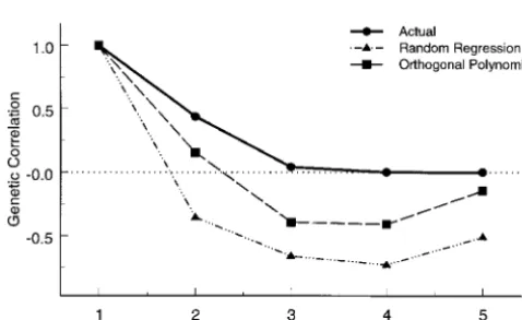
RESULTS correlation patterns that decrease asymptotically to zero
within the range of the data, and the correlation obtained
Simulations:For the stationary CP data, the best
ran-by both models goes negative (Figure 2). dom regression model according to the BIC criterion
The aim of the second simulated data set was to investi-was characterized by quadratic and linear deviations
gate the behavior of these models in the case of a rather for the genetic and environmental parts, respectively.
simple nonstationary genetic correlation structure. The Higher-order polynomials did not converge to a
maxi-best RR and OP models were the same as for the stationary mum and could not be considered. The best OP model
CP data detailed in the previous paragraph. The RR model contained a cubic polynomial for the genetic covariance
dealt very poorly with the nonstationary pattern of the and a quadratic for the environmental part. As expected,
genetic correlation (rc ⫽ 0.10); the correlation was esti-the simulated structure was accurately recovered by esti-the
mated to be very high over all ages. Again, the greater stationary character process model. Concordance
co-number of parameters in the best-fitting OP model over efficientsrcdescribing the goodness of fit for the
vari-the regression model provided a better fit to vari-the correla-ance and correlation functions are given in Table 1. For
tion structure (rc ⫽ 0.70). Surprisingly, the CP model the RR and OP models, the environmental covariance
failed to accurately estimate the nonstationary correlation structure (including both the variance and correlation)
pattern (Table 1). Our nonstationary extension did not was very well fitted (rc≈ 1). The genetic variance was
significantly improve the goodness of fit (BIC⫽ ⫺4454 also well modeled, but both models had trouble dealing
and⫺4456 for stationary and nonstationary models, re-with the rapidly decreasing genetic correlation function.
spectively;P⫽0.052 for a likelihood-ratio test of ⫽1.0). Although the OP model could better estimate the genetic
However, the goodness of fit of the fitted nonstationary correlation (rc⫽0.61 for OP compared to 0.36 for RR),
correlation (rc ⫽ 0.55) is substantially better than that it contains significantly more parameters than the
regres-of the stationary model (rc ⫽ 0.03), which provides an sion model (17vs.10), and both models exhibit similar
TABLE 1
Goodness-of-fit values for covariance functions estimated from three different methods on simulated data
Simulated covariance
structure Model VarG CorrG VarE CorrE BIC
Stationary CP CP 0.98 1.0 1.0 1.0 ⫺4591
RR 0.96 0.36 0.93 0.87 ⫺7414
OP 0.98 0.61 0.98 0.98 ⫺6605
Nonstationary CP CP 0.91 0.03 0.99 1.0 ⫺4454
RR 0.95 0.10 0.94 0.81 ⫺7397
OP 0.84 0.70 0.98 0.97 ⫺6628
Random regression CPa 1.0 0.93 0.96 0.93 ⫺3817
RR 1.0 0.94 0.99 1.0 ⫺3803
OP 1.0 0.94 0.99 1.0 ⫺3803
Orthogonal polynomial CPa 0.86 0.10 0.69 0.94 ⫺14334
RR 0.30 0.15 0.94 0.90 ⫺14371
OP 0.99 0.83 0.99 1.0 ⫺14272
Concordance values (seeappendix) for covariance functions estimated by three different methods on four representative covariance structures. The methods are CP, the character process model; RR, the random regression model; and OP, the orthogonal polynomial model. VarG represents the fit to age-specific genetic variances; CorrG refers to the fit to genetic correlations between ages; VarE represents the fit to environmental variances; and CorrE shows the fit to environmental correlations between ages. See text for details of the simulated covariance structures and details of the best-fitting models for each approach.
aThe best-fitting correlation function was a nonstationary CP model.
retrospect, the nonstationarity in this data set was predomi- netic and environmental) remained quite high over time. Our nonstationary extension of the CP model was success-nantly between extreme ages (ages 1 and 5). It is possible
that more observations per individual are needed to detect ful in providing a good fit to the data. The genetic covari-ance structure was described by a quadratic varicovari-ance and small to moderate levels of nonstationarity (see fly
repro-duction data). The genetic variance function and environ- nonstationary correlation given by the characteristic func-tion of the Uniform distribufunc-tion (PletcherandGeyer mental covariance structure were identical to that for the
1999), and the environmental variance function was linear stationary CP data and were well fit by all the methods
with a Cauchy correlation. The goodness of fit for the (Table 1).
genetic correlation structure was improved substantially All methods did a reasonable job of estimating the
over a stationary model (rc ⫽ 0.74, BIC ⫽ ⫺3819 and genetic and environmental covariance structures
gener-rc⫽0.93, BIC⫽ ⫺3817 for the stationary and nonstation-ated according to a random regression model with linear
ary CP models, respectively). deviations. Under this model the correlations (both
ge-Although we have essentially no idea what a typical age-dependent genetic covariance function might look like, the data set simulated with an OP structure might be considered pathological in that the genetic covariance structure is highly irregular. In fact, the genetic correlation is negative between early ages but highly positive between late ages (Figure 1D). Such a structure is, however, typical for OP models (Kirkpatrick et al. 1994). Convergence problems hindered our ability to obtain estimates of high dimensional random regression models, and the best RR model was not able to accommodate either the simulated genetic variance or correlation (rc⫽0.30 andrc⫽0.15, respectively). Both the genetic and environmental covari-ance structures were described by a quadratic varicovari-ance and nonstationary correlation given by the characteristic
Figure2.—Genetic correlations between age 1 and other function of the Uniform distribution. When compared for the simulated stationary character process data and fitted
to random regression, the CP model is much better at
genetic correlations obtained from the random regression
estimating the genetic variance function but is slightly
model with linear deviations and orthogonal polynomial of
TABLE 2
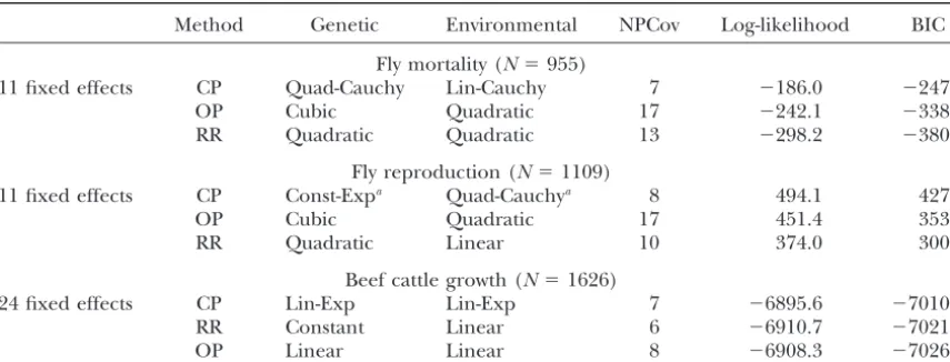
Results of covariance function estimation on empirical data
Method Genetic Environmental NPCov Log-likelihood BIC
Fly mortality (N⫽955)
11 fixed effects CP Quad-Cauchy Lin-Cauchy 7 ⫺186.0 ⫺247.7
OP Cubic Quadratic 17 ⫺242.1 ⫺338.0
RR Quadratic Quadratic 13 ⫺298.2 ⫺380.4
Fly reproduction (N⫽1109)
11 fixed effects CP Const-Expa Quad-Cauchya 8 494.1 427.5
OP Cubic Quadratic 17 451.4 353.4
RR Quadratic Linear 10 374.0 300.5
Beef cattle growth (N⫽1626)
24 fixed effects CP Lin-Exp Lin-Exp 7 ⫺6895.6 ⫺7010.0
RR Constant Linear 6 ⫺6910.7 ⫺7021.4
OP Linear Linear 8 ⫺6908.3 ⫺7026.4
The best-fitting genetic and environmental covariance functions for three different methods using empirical data on fruit fly mortality and reproduction and growth in beef cattle. Also presented is the log-likelihood of the models at their maximum and the BIC model selection criterion. NPCov represents the number of estimated parameters in the covariance structure for each model. The number of fixed effects reflects the number of different ages at which observations were obtained, andNis the total number of observations. Quad, quadratic; Const, constant; Exp, exponential; Lin, linear.
aThe best-fitting correlation function was a nonstationary CP model.
1). The environmental covariance is better behaved and This is true for reproductive output as well, and the sig-nificant nonstationary parameter in the genetic correla-much less of a problem. As seen with the random
regres-tion provides evidence for an increase in the correlaregres-tion sion simulations, the strong positive correlations across all
between two equidistant ages with increasing age. ages are well fit by all the methods.
Beef cattle:Although differences in fit among the
meth-Empirical:Drosophila reproduction and mortality:For
age-ods are less dramatic for beef cattle than for Drosophila, specific mortality and reproduction in Drosophila, the
the character process model again provides a significantly character process model provided a significantly better fit,
better fit (as determined by the BIC criterion) than either according to the BIC criterion, than either the orthogonal
random regression or orthogonal polynomial methods polynomial or random regression methods (Table 2). In
(Table 2). The best-fitting model for the genetic part was fact, the CP models achieved higher likelihoods despite
a linear variance (increasing with age) and an absolute containing significantly less parameters than the OP or
exponential correlation (G(ti, tj) ⫽ |ti⫺tj|)). There was
RR models. For age-specific mortality, the best-fitting
no evidence for nonstationarity in the data. Parameter model for the genetic covariance was a quadratic variance
estimates and their standard errors for the CP model are with a Cauchy correlation function (G(ti, tj)⫽ 1/(1 ⫹
presented in Table 3, and the fitted genetic covariance (ti⫺tj)2)). For fly reproduction the best character process
structure is shown in Figure 3C. model was a constant variance at all ages coupled with a
nonstationary correlation function described by the abso-lute exponential, G(ti, tj)⫽ |f(ti)⫺f(tj)|(see text following
DISCUSSION
Equation 5). Parameter estimates and their standard
er-rors for the CP model are presented in Table 3, and the The quantitative genetic analysis of repeated measures fitted genetic covariance structures are presented in Figure and other function-valued traits requires the estimation
3, A and B. of continuous covariance functions for each source of
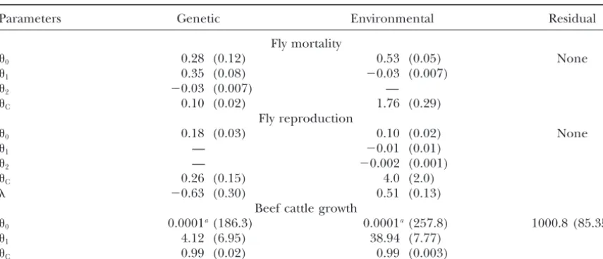
TABLE 3
Character process model estimates of genetic and environmental covariance functions for empirical data
Parameters Genetic Environmental Residual
Fly mortality
0 0.28 (0.12) 0.53 (0.05) None
1 0.35 (0.08) ⫺0.03 (0.007)
2 ⫺0.03 (0.007) —
C 0.10 (0.02) 1.76 (0.29)
Fly reproduction
0 0.18 (0.03) 0.10 (0.02) None
1 — ⫺0.01 (0.01)
2 — ⫺0.002 (0.001)
C 0.26 (0.15) 4.0 (2.0)
⫺0.63 (0.30) 0.51 (0.13)
Beef cattle growth
0 0.0001a(186.3) 0.0001a(257.8) 1000.8 (85.35)
1 4.12 (6.95) 38.94 (7.77)
C 0.99 (0.02) 0.99 (0.003)
Parameter estimates (and standard errors) for the best-fitting character process models for empirical data on fruit fly mortality and reproduction and growth in beef cattle.0,1, and2represent parameters of the variance function such that a quadratic variance is represented asv2(t)⫽
0⫹ 1t⫹ 2t2. In cases where the best-fitting model was constant or linear, the appropriate i are omitted. C and are parameters of the correlation function. A residual term is not always added in the model.
aParameter estimate is at the lower boundary and asymptotic standard errors may not be reliable.
process theory (i.e., the character process model) have mentioned previously, for random regression models the entire covariance structure is implicitly determined by the provided important alternatives. Other types of random
regression models (e.g., nonlinear models as suggested by shapes of the regression polynomials, and covariance sur-faces described by orthogonal polynomials have a fixed LindstromandBates1990 andDavidianandGiltinan
1995) may prove useful, but they are currently difficult to relationship between variance and correlation. This limita-tion is exemplified in the analysis of growth in beef cattle. implement.
Through extensive investigation of a variety of simulated For the genetic deviation, the best-fitting RR model in-cluded only a random intercept. This implies not only covariance structures and empirical data, we find that
under most conditions the CP models provide the best that the variance is considered constant over time but also that the correlation is constant and equal to 1 across all description of the underlying covariance structure. It is
clear from the simulation results that the CP model is the ages, which is probably not appropriate (Figure 3C). Applying the same argument to the fertility data in Dro-only method that adequately captures a correlation that
declines rapidly to zero as character values become further sophila, the best-fitting CP model for the genetic part was a constant variance with a rather rapid decline in separated in time. Both random regression models and
orthogonal polynomials have noticeable problems approx- correlation between increasingly separated ages (Table 3). Such a combination is simply not possible under the RR imating such a structure (Table 1, stationary CP data;
Figure 2). Polynomials do not have asymptotes, and the or OP methods. It is also likely that the separation of variance and correlation was a major factor contributing rapid decline in correlation tends to force both methods
to estimate correlations that are strongly negative within to the ability of the CP model to reasonably estimate the genetic variation with a much smaller number of parame-the range of parame-the data. Although parame-the characteristics of
covariance functions for natural organisms remain gener- ters (4 parameters) than random regression (10 parame-ters) or orthogonal polynomial (17 parameparame-ters) models ally unknown, this is a serious limitation as asymptotic
behavior in covariances/correlations are to be expected (Table 2).
The data sets we examined were small in comparison (PletcherandGeyer1999). Other parameterizations of
the RR models (e.g., using orthogonal polynomials in the to those commonly analyzed in agricultural and breed-ing contexts. Usbreed-ing extremely large data sets, compli-regression) may prove more useful in this regard. On the
other hand, RR and OP models work quite well when cated covariance and correlation models may be of greater use, and the random regression and orthogonal the correlation structure remains high over time (see
Ta-ble 1, environmental correlation in CP simulated data). polynomial methods may begin to show an advantage. Large data sets would also relieve the convergence prob-A further advantage of the CP models appears to be the
regres-several important limitations of the process models that suggest avenues for further development. First, addi-tional ways of relaxing the stationarity assumption (PletcherandGeyer1999) without greatly increasing the number of parameters are needed. Although not appropriate in all situations, a promising direction pro-posed by Nunez-Anton and Zimmerman (2000) has been studied here and seems to offer reasonable flexi-bility in practice. Second, CP models require the manip-ulation (inversion, factorization, etc.) of matrices whose dimensions are proportional to the number of ages in the data set, regardless of the size of the model itself (Meyer1998). A method of reparameterization, similar to that used for RR and OP models (Meyer 1998), would be useful. Third, a method for estimating the eigenfunctions of covariance functions used by the pro-cess models would provide insight into patterns of ge-netic constraints across ages (Kirkpatricket al. 1990; KirkpatrickandLofsvold1992).
Last, the genetic analysis of two or more function-valued traits is an important goal. Generalization of regression models to multitrait analyses is straightfor-ward and has already been used, for instance, to analyze age-dependent milk production, fat, and protein con-tent in dairy cattle (Jamrozik et al. 1997a). Bivariate character process models might be implemented by de-fining a parametric cross-covariance function between the two traits, but appropriate forms for this function are yet to be discovered.
W. Hill, N. Barton, and two anonymous reviewers provided valuable comments on the manuscript. Thanks to J. Curtsinger and A. Khazaeli for generously providing published and unpublished data. F.J. thanks the INRA for support during this project.
LITERATURE CITED
Davidian, M.,andD. M. Giltinan,1995 Nonlinear Models for Repeated Measurement Data.Chapman and Hall, London.
Diggle, P. J., K. Y. LiangandS. L. Zeger,1994 Analysis of Longitudi-nal Data.Oxford University Press, Oxford.
Gilmour, A. R., R. Thompson, B. R. CullisandS. J. Welham,1997
ASREML Manual.New South Wales Department of Agriculture, Orange, 2800, Australia.
Jamrozik, J., L. Schaeffer, Z. LiuandG. Jansen,1997a Multiple trait random regression test day model for production traits. Proceedings of 1997 Interbull Meeting, Vol. 16, pp. 43–47.
Figure3.—Contour plots of genetic covariance functions Jamrozik, J., L. R. SchaefferandJ.-C. M. Dekkers,1997b Genetic
fitted by the character process model. (A) Age-specific mortal- evaluation of dairy cattle using test day yields and random
regres-ity in the fruit fly,Drosophila melanogaster; (B) age-specific re- sion model. J. Dairy Sci.80:1217–1226.
Kirkpatrick, M.,andN. Heckman,1989 A quantitative genetic
production inD. melanogaster, (C) age-specific growth in beef
model for growth, shape, reaction norms, and other
infinite-cattle.
dimensional characters. J. Math. Biol.27:429–450.
Kirkpatrick, M.,andD. Lofsvold,1992 Measuring selection and constraint in the evolution of growth. Evolution46:954–971.
Kirkpatrick, M., D. LofsvoldandM. Bulmer,1990 Analysis of
sion and orthogonal polynomial models. Unfortunately, the inheritance, selection and evolution of growth trajectories. most quantitative genetic studies of natural and experi- Genetics124:979–993.
Kirkpatrick, M., W. G. HillandR. Thompson,1994 Estimating
mental populations are extremely labor intensive, and
the covariance structure of traits during growth and ageing,
illus-sample sizes will often be similar to those reported here. trated with lactation in dairy cattle. Genet. Res.64:57–69. For these situations, the properties of the character pro- Lindstrom, M. J.,andD. M. Bates,1990 Non-linear mixed effects
models for repeated measures data. Biometrics46:673–687.
cess models (e.g., easy hypothesis testing, few and
inter-Lynch, M.,andB. Walsh,1998 Genetics and Analysis of Quantitative
pretable parameters) make it a useful option. Traits.Sinauer Associates, Sunderland, MA.
Meyer, K,1998 Estimating covariance functions for longitudinal
data using a random regression model. Genet. Sel. Evol.30:
rc⫽1⫺ R
T⫺1
i⫽1 RTj⫽i⫹1(yij⫺yˆij)2
Ri,j(yij⫺y)2⫹Ri,j(yˆij⫺yˆ)2⫹T(T⫺1)(y⫺yˆ)2/2
,
221–240.
Meyer, K.,andW. G. Hill,1997 Estimation of genetic and
pheno-(A1)
typic covariance functions for longitudinal or ‘repeated’ records by Restricted Maximum Likelihood. Livest. Prod. Sci.47:185– 200.
where yˆij represents the estimated correlation between
Nunez-Anton, V.,1998 Longitudinal data analysis: non-stationary
error structures and antedependent models. Appl. Stochastic timestiandtjgiven by the model andyijis the correlation Models Data Anal.13:279–287.
between timestiandtjin the simulated data.Trepresents
Nunez-Anton, V.,andD. L. Zimmerman,2000 Modeling
non-sta-the total number of times at which measurements were
tionary logitudinal data. Biometrics56(in press).
Pletcher, S. D.,andC. J. Geyer,1999 The genetic analysis of age- taken.yandyˆare the means of the correlation values dependent traits: modeling a character process. Genetics153:
for the simulated data and for the model, respectively.
825–833.
The concordance coefficient for the variance estimate
Schwarz, G.,1978 Estimating the dimension of a model. Ann. Stat.
6:461–464. is much simpler and given by
Stram, D. O.,andJ. W. Lee,1994 Variance components testing in the longitudinal and mixed effects model. Biometrics50:1171– 1177.
rc⫽1⫺
RT
i⫽1(yi⫺ yˆi)2
Ri(yi⫺y)2⫹Ri(yˆi⫺yˆ)2 ⫹T(y⫺yˆ)2
, (A2)
Vonesh, E., V. ChinchilliandK. Pu,1996 Goodness-of-fit in gener-alized nonlinear mixed-effects models. Biometrics52:572–587.
Communicating editor:C. Haley
where the y’s now refer to the actual and estimated variances rather than correlations.
APPENDIX: GOODNESS OF FIT OF THE The coefficientrcis directly interpretable as a concor-COVARIANCE STRUCTURE
dance coefficient between observed and predicted val-ues. It directly measures the level of agreement (concor-The concordance correlation coefficientrcdescribed
dance) between yij andyˆij, and its value is reflected in
byVoneshet al.(1996) was used in the simulation study
how well a scatter plotyijvs. yˆijfalls about the line identity.
to evaluate the goodness of fit for both the variance
The possible values ofrcare in the range⫺1ⱕrcⱕ1, and correlation functions estimated by the models when
with a perfect fit corresponding to a value of 1 and a compared to the simulated structure. For the