Super-Diffusive Behavior in Human Mobility and Finding Relevant Models in Mobile Opportunistic Networks.

(1)

ABSTRACT

KIM, SUNGWON. Super-Diﬀusive Behavior in Human Mobility and Finding Relevant Models in Mobile Opportunistic Networks. (Under the direction of Professor Do Young Eun.)

Mobility is the most important factor in mobile ad-hoc networks (MANETs) and delay-tolerant networks (DTNs), and has posed a serious challenge to the analysis and design of protocols on such networks. The mobility pattern directly impacts time-varying contact/inter-contact dynamics among mobile nodes, which in turn aﬀects the perfor-mance of any protocol built over these mobility patterns. Mobility models that fail to capture key characteristics in the movement patterns of mobile nodes will result in mis-leading guidelines on the design of new protocols and evaluations of their performance and thus prevent us from making a right decision on our choice.

(2)

when diﬀusive properties are not properly captured. These results collectively suggest that the diﬀusive behavior of mobile nodes should be correctly captured and taken into account for the design and comparison study of network protocols.

(3)

Super-Diﬀusive Behavior in Human Mobility and Finding Relevant Models in Mobile Opportunistic Networks

by Sungwon Kim

A dissertation submitted to the Graduate Faculty of North Carolina State University

in partial fulﬁllment of the requirements for the Degree of

Doctor of Philosophy

Computer Engineering

Raleigh, North Carolina

2011

APPROVED BY:

Dr. Arne Nilsson Dr. Wenye Wang

Dr. Alun Lloyd Dr. Do Young Eun

(4)

DEDICATION

To my parents

(5)

BIOGRAPHY

(6)

ACKNOWLEDGEMENTS

Firstly, I would like to thank my advisor Dr. Do Young Eun. It was truly my honor and privilege to receive his guidance on research during my M.S. and Ph.D study at North Carolina State University. Dr. Eun has consistently encouraged and inspired me by recommending the best research directions and showing me the big pictures on research topics. He has motivated me to make the best eﬀort to pursue the high quality research, but he has been always forgiving. Thanks to his support and dedication, I could become a much better and conﬁdent researcher.

I also thank Dr. Arne Nilsson, Dr. Wenye Wang and Dr. Alun Lloyd, for being my advisory committee members. They were always willing to spend time on giving me useful suggestions on my research.

I have been very fortunate to have worked in Dr. Eun’s group with Dr. Xinbing Wang, Dr. Yuh-Ming Chiu, Dr. Han Cai, Terrence van Valkenhoef, Chul-Ho Lee, Dae-hyun Ban, Boonyarith Saovapakhiran, Xin Xu and Jaewook Kwak. I would like to give my special thanks to Chul-Ho Lee who collaborated with me on several works and spent lots of time in heated discussions for research topics.

(7)

LIST OF TABLES

Table 3.1 Summary of GPS traces . . . 19

Table 3.2 Summary of AP-Based traces . . . 27

Table 3.3 Notations and deﬁnitions used in Chapter 3.3 . . . 34

Table 3.4 Estimated MSD exponents γ using GCTRW(µ, β, p) . . . 42

Table 3.5 Summary of model T parameters . . . 57

(10)

LIST OF FIGURES

Figure 1.1 Various scenarios in mobile network. (a) Traditional one source and destination pair case; (b) Service provider content update case; (c) Multi-source content update case. Each mobile node A, B, C updates diﬀerent type of contents (e.g., news, weather forecast and traﬃc info). . . 6

Figure 2.1 MSD computation and sample trajectories of two nodes with dif-ferent diﬀusive properties. Two nodes moving with the same con-stant speed (1.34 m/s) are simulated over the same duration (10000 sec). . . 11 Figure 3.1 MSD of human mobile nodes. In all cases, MSD increases faster

than linear (super-diﬀusive behavior). . . 20 Figure 3.2 Mean Square Displacement (MSD) of the existing synthetic

mo-bility models (a)–(c) and the L´evy walk models on a log-log scale. . . . 23 Figure 3.3 Isotropic random walk with step-length Li and turning angle θi.

{Li} are i.i.d. with probability density fL(l), and {θi} are i.i.d. with unif[0,2π]. . . 25 Figure 3.4 Illustration of properties/limitations of AP-based traces. Location

of mobile nodes are mapped to AP-coordinates whenever they are associated with APs and unknown otherwise. A is the location where a mobile node pauses. . . 28 Figure 3.5 UCSD Traces: (a) CCDF of session time (P{Tsession > t}); (b)

MSD (from 9AM) on a log-log scale. The inset is for the trace that started from 11AM. Power-law density of Tsession implies that

Tpause also follows a power-law with the same exponent, making the

MSD grow very slowly; (c) MSD after randomization of location of mobile nodes inside APs. The MSD exponents remain untouched after randomization when compared with Figure 3.5(b). . . 29 Figure 3.6 Dartmouth Traces: (a) CCDF of session time; (b) MSD on a

(11)

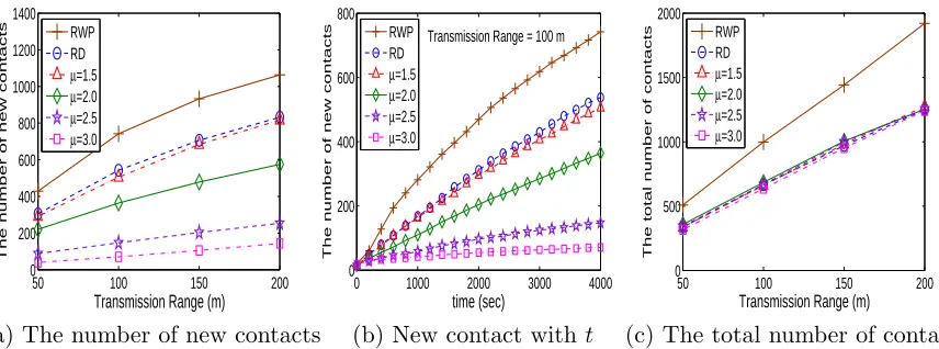
Figure 3.8 Impact of diﬀusive properties on contact-based metrics: (a) total number of new contacts among all nodes after simulation timet = 4000 seconds; (b) total number of new contacts during time interval t; (c) total number of contacts (including those among the same pair of nodes) after t = 4000 seconds. When µ is smaller (more frequent long steps), nodes tend to spread out further from the starting points, thus creating larger number of new contacts with other nodes. . . 47 Figure 3.9 Impact of diﬀusive properties on message delivery ratio for

differ-ent routing protocols. As the nodes tend to diffuse faster (smaller µ), the message delivery ratio becomes larger. This tendency holds for the performance of all six routing protocols. . . 49 Figure 3.10 Impact of diffusive properties on the performance of routing

proto-col with pause time considered. GCTRW(µ, β, p) model in Chapter 3.3, along with RWP and RD are used. While pause time induces longer message delivery, the ordering of performance is preserved as before. . . 50 Figure 3.11 Impact of diﬀusive properties on the performance of epidemic

rout-ing with different message TTL. The buffer size is set to 500 mes-sages. The ordering of performance results in Figure 3.9 is preserved. 51 Figure 3.12 Impact of diffusive properties on the performance of epidemic

rout-ing with different Buffer size B. The message TTL is set to 4000 seconds. The ordering of performance results in Figure 3.9 is pre-served. . . 52 Figure 3.13 Impact of diffusive properties on message delivery ratio for real

trace. Faster diffusive (µ = 0.80) nodes lead to higher message delivery ratio than slower diffusive (µ = 0.61). Note that pause time is included for the MSD slope in real trace. . . 53 Figure 3.14 Impact of diffusive properties on the number of new contacts and

delivery ratio in epidemic routing under a heterogenous mix of mobility models. Mobile nodes following Lévy walk model with µ = 1.5 and that with µ = 2.5 coexist. We vary the fraction of nodes following Lévy walk model with µ= 1.5 from 0 to 50, while keeping the total number of nodes the same (50 total). For exam-ple, legend “µ(1.5), µ(2.5)(40,10)” means that there are 40 nodes following Lévy walk with µ= 1.5 and 10 nodes withµ= 2.5. . . . 54 Figure 3.15 MSD measurement under Model T [34]. The AP locations at

(12)

Figure 4.1 Average age of contents with Poisson content update rate µ and contact rateλin service provider update case. Since service provider can directly distribute contents to every node, content update rate µplays a major role, and opportunistic contacts hardly contribute to freshness of contents whenµ is large. . . 64 Figure 4.2 Publish/subscribe case. Unlike the service provider update case,

the age of content at the publisher is not zero when one of the subscribers meets this publisher. . . 65 Figure 4.3 Average age of contents with Poisson update rate µ and contact

rate λ in publish/subscribe case. N is set to 50. For large λ/µ (µ ≤0.3 or λ ≥ 20 in Figures above), additional contacts (larger λ) hardly impact the average age. . . 67 Figure 4.4 A sample trajectory of Pearson walk (L=100m) and Random

di-rection model during 1000 sec. In Pearson walk, a mobile node moves straight with constant step lengthL m before it chooses the direction uniformly (and repeat), and in RD, a mobile node changes the direction at the boundary. . . 68 Figure 4.5 Average age of contents under Pearson walk with diﬀerentL. We

vary contact rate λ (0.0025 ∼ 0.017) by adjusting the number of nodes N from 10 to 70. . . 69 Figure 4.6 Average age of contents under L´evy walk model with diﬀerent µ.

We can observe the same trend as in Figure 4.5. . . 71 Figure 4.7 Age distribution forN = 50 in Pearson walk. Whenλ/µis larger,

the age distribution is almost identical to RD model. Note that for µ= 1 (×10−4), the age distribution is almost matched. The trend is almost identical to that of Figure 4.5. . . 72 Figure 4.8 Age distribution for N = 70 in Pearson walk. Comparing with

Figure 4.7, the difference of age distribution among different model is a lot more decreased sinceλ/µ is larger in this case. . . 73 Figure 4.9 Age distribution in Lévy walks for N = 50. . . 73 Figure 4.10 Age distribution in Lévy walks for N = 70. . . 73 Figure 4.11 Average age comparison between numerical results and theory. . 76 Figure 4.12 Rule of thumb on validity of ODE-based description. For largeλ/µ

regime, mobility models do not play a role on freshness of contents. Note that diﬀusive property of mobility model decides the slopea. 77

(13)

(14)

Chapter 1 Introduction

Mobility is the most important factor in mobile ad-hoc networks (MANETs) and delay-tolerant networks (DTNs), and has posed a serious challenge to the analysis and de-sign of protocols on such networks. The mobility pattern directly impacts time-varying contact/inter-contact dynamics among mobile nodes, which in turn aﬀect the perfor-mance of any protocol built over these mobility patterns [12]. Mobility models that fail to capture key characteristics in the movement patterns of mobile nodes will result in misleading guidelines on the design of new protocols and evaluations of their performance and thus prevent us from making a right decision on our choice.

(15)

approach is to rely on real mobility traces [1] and use them as inputs to a simulator for the study and comparison of protocols [44, 76]. This approach, however, suffers from lack of the amount of available traces on a fine time/space scale; most existing traces show only partial or ‘filtered’ information about the real trajectories of mobile nodes such as access point (AP) association information or just contact duration with others, not the actual spatial-temporal information of the mobile users on a fine scale. While [44, 76] have tried to extract meaningful metrics and reconstruct detailed mobility patterns out of those filtered traces using some heuristic algorithms, such reconstructed traces are applicable only for the particular setting under consideration (e.g., the same campus) and are highly sensitive on the choice of the reconstruction algorithm.

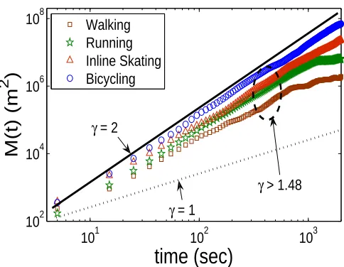
In this dissertation, we observe ‘super-diffusive’ movement pattern in mobility traces as a key property in human mobility, and study its impact on network performance extensively. By investigating the location of mobile nodes, and how it changes over time, we find that there is a common and distinctive characteristic observed in all mobility traces, super-diffusive movement pattern, which is characterized by a ‘faster-than-linear’ growth curve of the mean square displacement (MSD). The mean square displacement (MSD) – average square distance traveled by a mobile node over time durationt– can be used easily to quantify the diffusive property both in synthetic models and mobility traces, and does not require the accurate location coordinates of mobile nodes to find diffusive property. We use all the available GPS traces as well as AP-based traces to investigate the diffusive property in human mobility, and super-diffusive property is observed in all cases. Our findings are also in line with recent results in other scientific disciplines where almost all other living organisms invariably display super-diffusive property.

(16)

step-length exponent and the MSD slope in this model, and thus we can control the diﬀusive property easily by adjusting the step-length exponent.

Then, we provide the results that show how varying degrees of diffusive properties affect the characteristics of several contact-based metrics and simulation results for net-work performance evaluation via various routing protocols by using a set of Lévy walk models. We consider various scenarios by adding pause time, limiting resources (e.g., buffer size and TTL), and observe the huge impact of diffusive property consistently in all different scenarios.

(17)

models under single message scenarios.

1.1 Super-diﬀusive Behavior of Mobile Nodes and

its Impact on Routing Protocols

To find out key characteristics in movement patterns of mobile nodes, we first investi-gate numerous GPS-based mobility traces as well as AP-based traces. Unlike previous approaches using mobility traces, we specifically focus on the location of mobile nodes and how it changes over time. We then find that there is a common and distinctive characteristic observed in all mobility traces, super-diffusive movement pattern, which is characterized by a ‘faster-than-linear’ growth curve of the mean square displacement (MSD), i.e., E{∥Zt−Z0∥2} ∼ O(tγ) with γ > 1, where Zt ∈ R2 is the position of the mobile node at time t. The mean square displacement (MSD) – average square distance traveled by a mobile node over time durationt – is non-parametric and does not require any a priori specific mobility model for test, and is robust against the noise/error in the coordinates of mobile devices and the granularity of measurement time.

(18)

one-to-one relation between the exponent of the step-length distribution and the MSD slope, we can easily control the diﬀusive property through L´evy walk model in performance evaluation.

In particular, for AP-based traces, we show that there is a way to extract the diffusive property of mobile nodes in AP-based traces where location information Zt of a mobile node is spatially quantized (to coordinates of APs) and sporadically time-sampled only when mobile nodes get inside the range of an AP. By capturing the tail behavior of the pause time of mobile nodes and with the help of the continuous time random walk (CTRW) formalism, we set out to extract key characteristics of the mobility patterns again from MSD measurements. Specifically, we analytically show that under the class of CTRW models, a class of Lévy walk models interspersed with power-law distributed pause time can easily capture diffusive behavior observed in various AP-based traces.

(19)

1.2 Age Invariant Regime for Multi-Source Content

Update in Mobile Opportunistic Networks

Source

Destination

Service Provider

(a)

(b)

(c)

Pair wise contact rate

P

λ

update rate

µA

A

C

B

µB

µC Traffic

Weather

Breaking News

Figure 1.1: Various scenarios in mobile network. (a) Traditional one source and destina-tion pair case; (b) Service provider content update case; (c) Multi-source content update case. Each mobile node A, B, C updates diﬀerent type of contents (e.g., news, weather forecast and traﬃc info).

(20)

other subscribers. In this publish/subscribe paradigm, it is more reasonable to assume that subscribers would receive messages frequently from the publisher, so we would be in-terested in how fresh the contents are, or the ‘age’ of the contents. Also, in this scenario, all the mobile nodes in the network can be subscribers of contents.

There are several recent literatures that have focused on the age of contents, but in a different context. In [22], it is assumed that mobile nodes belong to one class depending on the spatial location, and move between classes in content update scenario. However, in this work, the specific mobility models that are used in many literatures have not been studied. In our work, by using several key mobility models, we investigate the age dynamics and the degree of impact depending on mobility models. [32] has studied the optimal allocation and scalability in mobile network where the freshness of contents matters. In this work, a single service provider, which can communicate directly with all the mobile nodes in the network, updates contents, and opportunistic contacts among mobile nodes are used to share more recent contents as briefly illustrated in Figure 1.1(b). In contrast, in our publish/subscribe scenario as shown in Figure 1.1(c), each and every mobile node updates its own content. Thus, a mobile nodeiacts like an individual service provider that generates a sequence of contents of type i with different time stamps and wants to get updated by all other types of contents via opportunistic contacts only. This scenario would be more realistic and useful in the future due to the fast growing users with portable communication devices and the development of social community that shares various information.

(21)

obtained via a simple ordinary diﬀerential equation (ODE) in terms of the average content update rate µ and contact rate λ among mobile nodes, by modiﬁcation of the results in [22]. We compare the age dynamics in our publish/subscribe case with that under the single service provider update case, and observe that there exists an age-invariant regime in which more frequent content updates or contacts among mobile nodes hardly contribute to the average age of the contents in both cases and specify this regime in terms of the ratio of content update rate µto contact rate λ. Interestingly, we observe a sharp contrast of age-invariant regimes in two cases.

(22)

ODE-based description can be conveniently used to predict the average age and discuss any deviation from ODE solution in some mobility models.

We also compare the publish/subscribe scenario with single message scenario in depth. We first enumerate the differences of these two scenarios and characterize each scenario in various aspects (e.g., metric, relevant scenario, viable applications). Then, by using the same simulation setup, we show that the impact of mobility models can be minimal in publish/subscribe scenario, which is not the case in the single message scenario. This finding is a sharp contrast to many previous works that have mainly focused on the impact of mobility models.

1.3 Organization

(23)

Chapter 2 Preliminaries

In this chapter, we ﬁrst present background on the mean square displacement – a metric to capture the rate at which mobile nodes spread out, and the super-diﬀusion. We then give notations, assumptions and the metric of interest in content update scenario. Finally, we summarize the related works.

2.1 Super-Diﬀusive Property

2.1.1 Mean Square Displacement (MSD)

One way to characterize the movement of a mobile node is to measure how far it is away from its current position after time t. This ‘diffusive’ behavior or the rate at which the mobile node spreads out can be described and quantified by so-called the mean square displacement (MSD) [15, 68, 69]. Specifically, if we define Zt ∈ R2 to be the position of the mobile node at time t, then the MSD becomes M(t), E{∥Zt−Z0∥2}, (i.e., the

second moment of the displacement ∥Zt−Z0∥ between the current position at time t

(24)

X Y

t₃ t₂

t₁

Z3

Z1

Z2

(0,0)

−1000 −500 0 500 1000 −1000

−500 0 500 1000

X(m)

Y(m)

Normal diffusive (γ=1.0) Super diffusive (γ=1.5)

(a) MSD computation (b) Super-diﬀusive node

Figure 2.1: MSD computation and sample trajectories of two nodes with diﬀerent diﬀu-sive properties. Two nodes moving with the same constant speed (1.34 m/s) are simulated over the same duration (10000 sec).

mobile node after time t. For example, for a class of isotropic random walks with ﬁnite step-length1 _{variance, the MSD will grow linearly with} _t_{, i.e.,} _M₍_t₎ _∼ _t_{, provided that}

the speed of the mobile node is O(1) (or constant).2 _{In general, we have} _M₍_t₎_∼ _O₍_tγ₎ for some γ > 0. The slope of M(t) in a log-log scale (γ) characterizes how fast a node spreads out in a simple way. Figure 2.1(a) shows how MSD can be measured. In this ﬁgure, as the mobile node starting from the origin follows the trajectory shown in dashed line, we can collect the displacement at each time instant ti and investigate how MSD grows with time t to uncover the diﬀusive property of mobile nodes.

2.1.2 Super-Diﬀusion

When the step-lengthLhas inﬁnite variance (σ2_L=∞), the mobile node tends to quickly spread out since longer step-lengths are generated more often. This behavior is called

(25)

super-diﬀusion [48, 69, 70, 81, 82], while for σ2

L < ∞ it is called normal diffusion. The varying degrees of diffusive properties of mobile nodes can be conveniently captured by the slope (γ) of M(t) in a log-log scale (i.e., M(t) ∼ tγ_{). For example, we have} γ = 1 for a normal diffusive case, while γ > 1 for super-diffusive case (faster-than-linear growth of the MSD). Figure 2.1(b) shows typical sample trajectories of two mobile nodes with different diffusive properties (different γ). While both nodes have the same constant speed (1.34 m/s) and run over the same duration (10000 sec), the super-diffusive node (γ = 1.5) spreads out from the origin much farther than the normal-diffusive node (γ = 1.0). As Figure 2.1(b) illustrates, the occasional long jumps are key characteristics of super-diffusive movement patterns.

2.2 Content Update Scenario

2.2.1 System description

(26)

2.2.2 Content update

User i (publisher) updates its content (type i) with rate µ. We denote by tsij(t) the time-stamp of typeicontent (originally generated from useri) that is currently stored in userj’s buﬀer at timet. In our publish/subscribe scenario, opportunistic contacts among mobile nodes are the only way to share contents with other nodes and keep them updated. Contact rate between useriandj is set toλp (here subscript indicates pairwise contact), while we use λ to denote the ‘aggregate’ contact rate per user, i.e.,λ= (N−1)λp when there are N mobile nodes in the network. When there is a contact between users i, j at time t, both of which having type k content (generated by user k) with time stamp tski(t) andtskj(t), respectively, they both update this content by sharing more fresh one with time stamp given by max{tski(t), tskj(t)} (and delete the old one from the buﬀer).

2.2.3 Age metric

To measure the freshness of contents, we need a proper metric. In this dissertation, we adapt the freshness metric defined in [32, 33]. For the type i content that is currently stored at node j with time stamp tsij(t), we define the age of the content as Aij(t) = t−tsij(t) for i, j ∈ S. Thus, the age of each content increases linearly with time and jumps down if the user contacts other users having fresher content (larger time stamp) of the same type. We then define the average age over all nodes and all content types as

A(N, t) = 1 N

N

∑

i=1

N

∑

k=1

Aki(t). (2.1)

(27)

2.3 Related Work

(28)

The mobility model has also been a central topic in other scientific disciplines and various attempts to explain the movement of living organisms in nature have been made [24, 47, 65]. In particular, the so-called Lévy walk model, whose defining char-acteristic is its super-diffusive property, has been adopted for modeling the movement patterns of living organisms such as Microzooplankton [14], seabirds (albatross) [78], reindeer [55], jackals [10], and monkeys [16, 58], as well as capturing their foraging pat-terns [67, 78, 79]. Anthropologists also have started to pay attention to Lévy walk pattern to analyze the mobility phenomenon in their field [17]. Quite recently, the super-diffusive behavior of mobile nodes has also received attention in representing human mobility pat-tern via a limited number of GPS-based traces [45, 61]. In contrast, in this dissertation, we investigate the vast amount of AP-based traces [1, 7, 56] (for which GPS-coordinate information is unavailable) through the CTRW formalism with heavy-tailed nodes’ pause time [76], and find that the super-diffusive behavior of nodes’ movement is a universal property in all the mobility traces under our study.

(29)

(30)

Chapter 3 Super-Diﬀusive Behavior of Mobile

Nodes and its Impact on Routing

Protocol Performance

There have been numerous approaches to find key characteristics in human mobility using mobility traces. Statistical information such as speed, pause time and inter-contact time of mobile nodes has been investigated in previous works [23, 27, 40, 44, 76] based on mobility traces and its impact on network performance is studied. In this chapter, we find super-diffusive property as key characteristic in human mobility. The mean square displacement (MSD) – average square distance traveled by a mobile node over time duration t – is used to measure diffusive property, and this metric is easy to use and robust against the noise/error in the coordinates of mobile devices and the granularity of measurement time.

(31)

models in the context of their diffusive properties, and introduce Lévy walk models as good candidates for producing various degrees of diffusive behavior. In Chapter 3.2, we investigate AP-based traces, and characterize the diffusive properties when pause time is included. In Chapter 3.3, we introduce CTRW and generalized MSD for a class of isotropic random walks with heavy-tailed pause time. In Chapter 3.4, we provide simu-lation and numerical results to show the impact of diffusive properties on contact-based metrics and network performance. We consider various scenarios with and without pause time, and change the resource constraints by adjusting the message TTL and buffer size. We also consider the different sets of diffusive mobility traces. In Chapter 3.5, we discuss the issue of other factors toward the super-diffusive property and how to incorporate the observed property in traces into the set of Lévy walk models. In addition, we show that even trace-based models can generate super-diffusive property.

3.1 Diﬀusive Behavior in GPS-based Traces and

Syn-thetic Models

In this chapter, we examine various GPS traces with different movement patterns and show all of them display the super-diffusive behavior. We then study whether the existing synthetic models can effectively capture the observed diffusive properties.

3.1.1 GPS Traces Validation

(32)

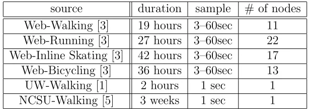
Table 3.1: Summary of GPS traces

source duration sample # of nodes Web-Walking [3] 19 hours 3–60sec 11 Web-Running [3] 27 hours 3–60sec 22 Web-Inline Skating [3] 42 hours 3–60sec 17 Web-Bicycling [3] 36 hours 3–60sec 13 UW-Walking [1] 2 hours 1 sec 1 NCSU-Walking [5] 3 weeks 1 sec 1

Available GPS Traces

Table 3.1 is the summary of GPS traces of human beings under our consideration for their diﬀusive properties. Below is the detail about the GPS traces sources.

www.gps-tour.info: [3] is a GPS device users’ community website where users

share GPS traces. This website has an extensive amount of data from about 50 countries for various activities. We use this as our main source of GPS traces.

University of Washington: The GPS trace of University of Washington (UW)

was collected by one of the authors in [39] for about two hours. This trace provides the x, y co-ordinates of the mobile node every second even inside of buildings by using Place Lab [6].

NCSU:NCSU GPS traces [5] were collected from the present authors’ school campus,

where one student carried a GPS device (Garmin eTrex [2]) to collect GPS traces.

Extracting MSD from GPS traces

(33)

we ﬁrst removed all the pause time in the GPS traces, and then computed MSD from the resulting traces.

101 102 103

102 104 106 108

M(t) (m

2 )

time (sec)

Walking

Running Inline Skating Bicycling

γ = 2

γ = 1

γ > 1.48

Figure 3.1: MSD of human mobile nodes. In all cases, MSD increases faster than linear (super-diﬀusive behavior).

(34)

3.1.2 Diﬀusive Behavior in Synthetic Models

In this part, we first study diffusive behavior in current synthetic mobility models via their MSD and show that most of them are not suitable for capturing varying degrees of super-diffusive pattern. We then propose to use a set of Lévy walk models as a simple alternative to current synthetic models.

Correlated Random Walks

Among existing synthetic mobility models, we first consider several correlated random walk models to see if they can capture super-diffusive behavior. Since a mobile node in a correlated random walk tends to move along the same (or similar) direction for a while before changing its direction, these models might be good candidates for capturing super-diffusive behavior. Here, we consider the following set of correlated random walk models currently used in MANET simulations.

Correlated Random Walk on Grid (CRWG): A two-dimensional correlated

random walk model on grid is proposed in [13] as a generalization of Manhattan mobility model [12]. In this model, a mobile node takes a step to the same direction as the previous one with probabilitypand opposite direction (moving backward) with probabilityq, while the probability of turning right or left isr satisfying p+q+2r= 1. By assigning diﬀerent values ofp, q, we can control the degree of tendency for a mobile node to follow the same direction.

Gauss-Markov Mobility Model: A Gauss-Markov mobility model [21] ﬁrst

(35)

follow Gaussian distributions. Speciﬁcally, the direction (turning angle) of the nth _step θn is updated as

θn =ρθn−1+ (1−ρ)¯θ+

√

(1−ρ2₎_θ

xn−1, (3.1)

where θxn

d

=N(0, σ2_{) are} _i.i.d. _{zero mean Gaussian with variance} _σ2_, _ρ _∈ _[0_,_{1] is the}

correlation coeﬃcient, and ¯θ is the preferred direction (angle). Step-lengthlnalso follows a similar recursion. We here consider a modiﬁed version of this Gauss-Markov model for fair comparison with other models in a way that after every t second, we update its step-length (instead of its speed) with its speed (1.34 m/s) and the preferred step-length (10m) kept the same all the time.

This Gauss-Markov model in (3.1) oﬀers a great deal of ﬂexibility by controlling the shape of distribution (σ) and correlation structure (ρ). For instance, whenρ≈1 andσ2

is small, the turning angles (θi in Figure 3.3) remain almost the same, thus the mobile node will follow a straight line for a very long time, while for ρ ≈ 0 and large σ the angle distribution approaches to a Gaussian with mean ¯θ and a large variance σ, but independent over time, thus is close to that of an isotropic random walk.

MSD of Correlated Random Walks

(36)

101 102 103 103 104 105 106 107 time (sec) M(t) (m 2)

( p=0.9, r=0.05 ) ( p=0.5, r=0.25 )

γ = 0.97

γ = 0.95

101 102 103

102 104 106 108 time (sec) M(t) (m 2)

σ=1, ρ=1

σ=1, ρ=0

σ=1, ρ=0.95

σ=2, ρ=0.95

σ=4, ρ=0.95

Slope: 2

Slope: 1

γ = 1.04

γ = 1.78

γ = 1.19

γ = 1.94 ~ 2

(a) CRWG (b) Guass-Markov

101 102 103

103 104 105 106 107 time (sec) M(t) (m 2 ) RWP RD

γ = 1.96 (RWP) 1.87 (RD)

101 102 103

102 104 106 108 time (sec) M(t) (m 2 ) µ=1.5 µ=2.0 µ=2.5 µ=3.0

γ = 1.04

γ = 1.46

γ = 1.78

γ = 1.95

(c) RWP, RD (d) L´evy walk

(37)

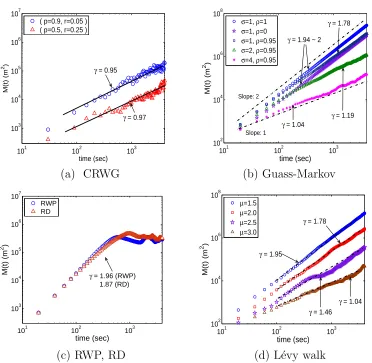
Figure 3.2(b) shows the MSD of Gauss-Markov mobility models with diﬀerent degrees of correlations (ρ) and variance σ2 _{of turning angle} _θ

n. For σ = 2,4, a mobile node tends to deviate from its preferred angle with varying degree of step-lengths, which all contribute to the linear growth rate of the MSD even when there exists considerable amount of correlationsρ= 0.95. On the other hand, as can be seen for the case ofσ = 1, Gauss-Markov model is likely to generate ‘ballistic’ trajectory (γ = 2) where the marginal angle distribution is ‘pointed’ with small σ (the mobile node has favorite direction and remembers this forever), and the MSD now grows much faster than linear. In all cases we see that σ plays a dominant role in shaping the angle distribution than the amount of correlation ρ, since the eﬀect of small σ persists in the turning angle (the mobile node remembers its preferred angle forever) while the eﬀect of correlations will be smoothed out over longer period as already seen in Figure 3.2(a).

To sum up, in order to capture the super-diffusive behavior with correlated walk models, one would have to tweak the distribution and correlations of the angles very carefully. As Figures 3.2(a) and 3.2(b) show, however, this approach would typically result in either γ ≈ 1 or γ ≈ 2, thereby making it unwieldy or practically infeasible to generate various mobility patterns with different degrees of diffusive behavior.

MSD of mobility models with boundary (RWP and RD)

(38)

back. Note that the timescale over which the node diﬀuses is much shorter than other models in Figure 3.2.

L´evy Walk model

L1

L2

L3

1

θ

2

θ

3

θ

0 0

( ,x y ) _X

Y

1 1

( ,x y)

2 2 ( ,x y)

Figure 3.3: Isotropic random walk with step-length Li and turning angle θi. {Li} are i.i.d. with probability density fL(l), and {θi} are i.i.d. with unif[0,2π].

A Lévy walk model is defined as follows. Suppose that a mobile node first chooses a step-length L and then moves that distance with some constant speed at an angle θ drawn uniformly and randomly from [0,2π] as illustrated in Figure 3.3. When it finishes that step-length, it repeats the process, independently of the past. When the first or the second moment of the step-length L becomes infinite, the model is called a Lévy walk [49, 68, 80]. For a Lévy walk model, the step-length density is characterized by

fL(l)∼l−µ, 1< µ <3,

(39)

mobility model, a mobile node occasionally moves along a very long straight line with non-negligible probability, interspersed with successive short steps with random orientation. Unlike other mobility models that would require subtle choice of several parameters to control diffusive properties, Lévy walk models can directly control the degree of super-diffusive properties by adjusting the exponent of step-lengths µ (single parameter) as shown in Figure 3.2(d).

3.2 Diﬀusive Behavior in AP-Based Traces

(40)

3.2.1 Available AP-Based Traces

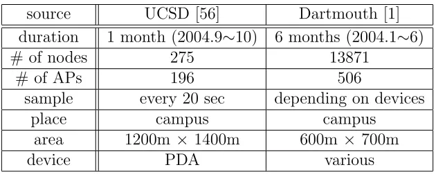
To verify diﬀusive properties in AP-based traces, we use two sets of data, University of California at San Diego (UCSD) traces [56] and Dartmouth College traces [1], for which AP-coordinates are available and they are most widely used in literatures. The summary of AP-based traces is given in Table 3.2.

Table 3.2: Summary of AP-Based traces

source UCSD [56] Dartmouth [1]

duration 1 month (2004.9∼10) 6 months (2004.1∼6)

# of nodes 275 13871

# of APs 196 506

sample every 20 sec depending on devices

place campus campus

area 1200m ×1400m 600m × 700m

device PDA various

To extract the data set that can well represent the mobility of nodes from the huge amount of traces in Table 3.2, we preprocessed the raw data. First, we used only weekday traces as the quantity of weekday traces is guaranteed to be large. Then, we considered the traces only after 9AM each day, as most mobile nodes start doing activities over this period. In order to rule out short-lived nodes leaving the network quickly, we only considered mobile nodes whose traces are at least 3 hours long.

3.2.2 MSD with Pause Time in AP-Based Traces

(41)

AP2

AP1

t1

t4

t3

t2

(path2)

(path1)

·

(x2, y2)

(x1, y

·

1)

t5

t6

A

Figure 3.4: Illustration of properties/limitations of AP-based traces. Location of mo-bile nodes are mapped to AP-coordinates whenever they are associated with APs and unknown otherwise. A is the location where a mobile node pauses.

node and for each AP with known coordinates (xi, yi), we know when the mobile node enters this AP (say, tj). By tracking this information of time instants and coordinates in an increasing order of tj, we can compute the distance a mobile node has traveled from its starting point for certain time duration. In other words, we can obtain sample values of the MSD and consequently its slope (γ) on a log-log scale.

In addition to the MSD samples, AP-based traces also contain some information about the pause time of each mobile node. As shown in Figure 3.4, a collection of intervals during which a node is associated with some AP (e.g., [t1, t2],[t3, t4], . . .), tells us how long

the node stays inside the range of an AP. This interval is often called a session time [76]. Note that one session time interval consists of actual amount of pause time (point A in AP2 in Figure 3.4) and the amount of time during which the mobile node keeps moving within the range of AP, i.e., Tsession = Tpause +Tmove. AP-based trace data reveal that

(42)

102 103 104 10−4 10−3 10−2 10−1 100 time (sec) CC DF

Slope = −0.38

103 104

104 105 time (sec) M( t) (m 2 )

γ = 0.65

103 104 104

105

γ = 0.61

103 104

104 105 time (sec) M( t ) (m 2)

γ = 0.64

103 104 104

105

γ = 0.61

(a) Session-Time (b) MSD from 9AM, 11AM (c) After randomization

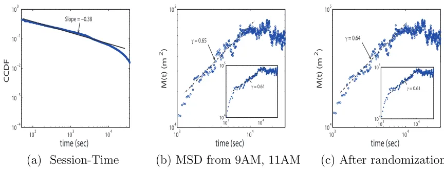
Figure 3.5: UCSD Traces: (a) CCDF of session time (P{Tsession > t}); (b) MSD (from

9AM) on a log-log scale. The inset is for the trace that started from 11AM. Power-law density of Tsession implies that Tpause also follows a power-law with the same exponent,

making the MSD grow very slowly; (c) MSD after randomization of location of mobile nodes inside APs. The MSD exponents remain untouched after randomization when compared with Figure 3.5(b).

large.1

Figure 3.5(a) shows that the CCDF of the session time in UCSD trace data follows a power-law with exponent around −0.38. The session time in Figure 3.5(a) is collected during the same period as in Figure 3.5(b). In these ﬁgures, we only consider session time samples up to 10 hours long, since the session time longer than 10 hours would be from devices that remain on but are not used for a long time. Note that the amount of sojourn time inside an AP due to movement (Tmove) has the same order as the ﬁrst

hitting time of a 2-D random walker to the perimeter of AP-disk starting from inside, whose distribution is known to be at most exponential [59]. This implies that the tail of the pause time probability density functionϕ(t) also follows a power-law ϕ(t)∼t−β _with

1_{A survey in [28] shows that the ratio between total moving time and total pause time (stationary}

(43)

103 104 10−4

10−3 10−2 10−1 100

time (sec)

C

CD

F

Slope=−0.23

103 104

time (sec)

M

(t) (m

2 )

γ = 0.69

103 104

103

104

γ = 0.60

(a) Session-Time (b) MSD from 9AM, 11AM

Figure 3.6: Dartmouth Traces: (a) CCDF of session time; (b) MSD on a log-log scale. Session time and diﬀusive behaviors are similar to those of UCSD traces in Figure 3.5.

β ≈1.38.

Figure 3.5(b) shows the sample values of the MSD M(t) over time t in a log-log scale using traces from 9AM. (All the inset ﬁgures are from 11AM.) During the time duration from 2000 to 10000 seconds (for about 2.5 hours), MSD of mobile nodes increases with γ ≈ 0.65. As expected, the existence of heavy-tailed pause time makes the MSD grow much slower compared with the case of GPS traces in Chapter 3.1.1.2 _{Unlike the GPS}

traces, however, it is impossible to extract the pause time component from the AP-based traces as mobile nodes do move around inside APs, whose component is subsumed into the session time as a whole. Nevertheless, later in Chapter 3.3, we will show that there is a way to infer the true diﬀusive behavior of mobile nodes from their movement components only and that it is again super-diﬀusive as is the case for GPS traces in Chapter 3.1.1.

Here we point out that the super-diﬀusive behavior captured by the super-linear growth ofM(t) should be addressed only on a relevant time scale, not necessarily over all

(44)

time t. For example, mobile nodes in school (students) spread out for a while and even-tually tend to come back to their starting points (e.g., dormitory, library or classroom). Indeed, Figure 3.1 shows that the typical timescale for the super-diﬀusive behavior is up to O(103_{) seconds, beyond which the mobile nodes display no further diﬀusive behavior}

or strong tendency to come back. Note that this timescale of several thousands of seconds is without the pause time, so with possibly very long pause time (e.g., several hours), the timescale for the diffusive behavior with pause time would have been prolonged. In both UCSD and Dartmouth traces, similar diffusive properties are observed in almost identical time scale 2000≤ t <10000 as shown in Figures 3.5(b) and 3.6(b). Note that the time scale 2000 ≤ t < 10000 can represent the overall diffusive property well since both movement diffusive property and pause time are fairly considered in this time scale regardless of the type of mobile devices. We also point out that the diffusive property over time scalet <2000 and t≥10000 is sensitive to the types of devices and user char-acteristics of traces. For example, PDA users are likely to start to move after they turn on the device, while laptop users3 tend to stay where they are right after they turn on the devices, which explains the different diffusive property for t < 2000. Beyond 10000 seconds, MSD tends to decrease or fluctuate around some value in both traces, which is due to the geographical constraints and/or the tendency of coming back to the starting point. However, note that the tendency of coming back to the same location that they have left in the morning for UCSD trace is stronger than Dartmouth trace, (All the users in UCSD traces are freshmen and most of them live in a dormitory.) which corresponds to different diffusive property over t≥10000.

In AP-based traces, since the exact coordinates of mobile nodes at each time t is

3_{Many diﬀerent types of mobile devices contribute to Dartmouth trace. Even though laptop is not the}

(45)

unavailable inside APs, we have simply assumed that the coordinate of an AP represents that of all mobile nodes within the communication range of APs. To justify this assump-tion, we did a simple experiment. First, we set the communication range r of one AP to 25m, which is reasonable considering the real wireless network. Then, we newly set the coordinate of each mobile nodes inside an AP to another randomly (and uniformly) chosen location inside the AP-circle of radius r. Figure 3.5(c) shows the MSDM(t) over time t after we randomize the locations of mobile nodes inside APs. Observe that the MSD exponents are largely unaﬀected by this randomization when compared with the original (non-randomized) version in Figure 3.5(b). To explain this behavior, let Zt be the original coordinate of a mobile node at time t and Nt be a stationary zero-mean random process in 2-D (independent of Zt) with E{∥Nt∥2} =σN2 <∞, representing the ‘noise’ in the coordinates of mobile nodes in our randomization procedure. Then, the ‘estimated’ location at time t becomes ˜Zt,Zt+Nt, whose MSD is in the form of

˜

M(t) = E{∥Zt+Nt∥2}=E{∥Zt∥2}+σ2N =M(t) +σ

2

N.

(46)

3.3 Continuous Time Random Walk (CTRW)

In Chapter 3.2, we showed diffusive properties of AP-based traces as is, with the pause time added. In this chapter, we introduce and utilize the general framework of CTRW [30, 49, 84] in order to uncover the true diffusive behavior of mobile nodes in AP-based traces without pause time. Specifically, we consider a class of isotropic random walks as depicted in Figure 3.3, but now we allow a mobile node to pause for a random amount of time with some probability p, independently of all others, at each turning point. Then, we present a set of equations to compute the MSD for this generalized CTRW (with heavy-tailed pause time) and identify under what conditions we can recover the observed the MSD growth rate of AP-based traces (as seen in Figures 3.5 and 3.6). Lastly, we confirm through theoretical and numerical results that a class of Lévy walk models interspersed with power-law pause time can effectively capture the diffusive behavior observed in the ‘filtered’ AP-based traces.

To set the stage, let P(⃗r, t) be the joint probability density for a node to be located at⃗r ∈ R2 if started from the origin at t = 0. We deﬁne by h(⃗r, t) the joint probability density that a node makes a displacement of ⃗r in a single step and this takes exactly t seconds. We further deﬁne by ϕ(t) the probability density of a pause time between successive steps. In particular, h(⃗r, t) can be written as h(⃗r, t) = f(⃗r|t)ψ(t), where ψ(t) is the probability density for the time duration of a single step and f(⃗r|t) is the conditional probability density that a node makes a displacement of⃗r in a single step for a given time duration t. For example, if the node moves around with constant speed v all the time, then f(⃗r|t) is in the form ofδ(∥⃗r∥ −vt) since the node can travel exactly vt meters during t seconds, where δ(·) is the Dirac delta function.

(47)

Table 3.3: Notations and deﬁnitions used in Chapter 3.3 Notation Deﬁnition

M(t) mean square displacement (MSD)

P(⃗r, t) joint probability density for a node to be located at⃗r∈R2 if started from the origin att = 0

fL(l) probability density of a step-length

ψ(t) probability density for the time duration of a single step f(⃗r|t) conditional probability density that a node makes a

displacement of⃗r in a single step for a given time duration t h(⃗r, t) joint probability density that a node makes a displacement

of⃗r in a single step and this takesexactly t seconds (h(⃗r, t) = f(⃗r|t)ψ(t))

H(⃗r, t) probability that a node makes a displacement of⃗r in time t within a single step and it takes at least t seconds to

complete a single step (H(⃗r, t) =f(⃗r|t)∫_t∞ψ(τ)dτ)

ϕ(t) probability density of a pause time between successive steps Φ(t) probability that a node has not moved until time t

(48)

denotes the probability that a node makes a displacement of ⃗r in time t within a single step and it takes at least t seconds to complete a single step (i.e., the probability that a node makes a displacement of ⃗r for time t and it does not necessarily stop to initiate a new step or to stay at time t). Thus, H(⃗r, t) can be written as f(⃗r|t)∫_t∞ψ(τ)dτ. In addition, Φ(t) denotes the probability that a node has not moved until time t, which is given ∫_t∞ϕ(τ)dτ. For reference, all the notations and deﬁnitions used in this chapter are summarized in Table 3.3.

We are interested in computingP(⃗r, t) as this provides complete information on where the node will be located at any given time t. The desired P(⃗r, t) can be obtained by summing over all the possible events. Note that a displacement of ⃗r in time t can be made by either a single step or multiple steps. Thus, by conditioning upon ﬁrst step taken, P(⃗r, t) can be decomposed into the following four (disjoint) cases:

(i) The node reaches⃗r in timet within its ﬁrst step without pause during [0, t].

(ii) The node reaches⃗r at some earlier time τ ∈ (0, t) in its ﬁrst step and stays there for a remaining timet−τ with probability p.

(iii) The node reaches ⃗ρ ̸= ⃗r at some earlier time τ ∈ (0, t) in its ﬁrst step, takes no pause time with probability 1−p, and then continues to move from ⃗ρ to reach ⃗r for a remaining timet−τ.

(iv) The node reaches ⃗ρ̸=⃗r at some earlier time τ′ ∈(0, t) in its ﬁrst step, takes pause time of τ −τ′ >0 with probabilityp, and then continues to move from ⃗ρ to reach ⃗r for a remaining time t−τ.

(49)

above, we arrive to the following recursive equation analogous to the backward equation of Chapman-Kolmogorov equation in the theory of Markov processes:

P(⃗r, t) =H(⃗r, t) +

∫ t

0

dτ h(⃗r, τ)p Φ(t−τ)

+

∫∫

R2

d2⃗ρ

∫ t

0

dτ h(⃗ρ, τ)(1−p)P(⃗r−⃗ρ, t−τ)

+

∫∫

R2

d2⃗ρ

∫ t

0

dτ

∫ τ

0

dτ′h(ρ, τ⃗ ′)pϕ(τ−τ′)P(⃗r−⃗ρ, t−τ), (3.2)

where H(⃗r, t) = f(⃗r|t)∫_t∞ψ(τ)dτ and Φ(t) =∫_t∞ϕ(τ)dτ.

Note that as we are interested in the location ⃗r of the node at any given time t, the node would be located at⃗r at timet during the movement of a single step or pause time, not necessarily to be the end of a single step or pause time. Thus, for the ﬁrst and second terms, H(⃗r, t) and Φ(t) are used instead ofh(⃗r, t) and ϕ(t), respectively.

As MSD is the second moment of the displacement ∥Zt−Z0∥ between the current

position at time t and the position at time 0 as deﬁned before, Fourier transform (i.e., characteristic function) could be a convenient way to derive MSD. We deﬁne by P(⃗ω,·) the Fourier transform (⃗r → ⃗ω) of P(⃗r,·), i.e., P(⃗ω,·) = ∫∫_R2P(⃗r,·)ei⃗ω⃗rd2⃗r. Thus, MSD

can be easily computed by taking the second derivative of P(⃗ω, t) and by evaluating it at⃗ω =⃗0, i.e.,

M(t) = −∂

2_P₍_⃗_{ω, t}₎

∂⃗ω2

⃗

ω=⃗0. (3.3)

Similarly, we take Laplace transform with respect to t (t → s) and deﬁne Pb(·, s) =

∫_∞

0 P(·, t)e−

(50)

and Laplace transforms exhibit the following convolution property:

∫∫

R2

[∫∫

R2

f(⃗ρ,·)g(⃗r−⃗ρ,·)d2⃗ρ

]

ei⃗ω⃗rd2⃗r =f(⃗ω,·)g(⃗ω,·),

and

∫ _∞

0

[∫ t

0

f(·, τ)g(·, t−τ)dτ

]

e−stdt =fb(·, s)bg(·, s),

where f and g are well-deﬁned functions.

Therefore, by taking Fourier-Laplace transform of (3.2) and exploiting the eﬃciency of the convolutional property, we obtain

b

P(⃗ω, s) =

∫ _∞

0

[∫∫

R2

P(⃗r, t)ei⃗ω⃗rd2⃗r

]

e−stdt

=Hb(⃗ω, s) +pbh(⃗ω, s)Φ(b s) + (1−p)bh(⃗ω, s)Pb(⃗ω, s)

+pbh(⃗ω, s)ϕb(s)Pb(⃗ω, s). (3.4)

Then, Pb(⃗ω, s) becomes

b

P(⃗ω, s) =

b

H(⃗ω, s) +pbh(⃗ω, s)Φ(b s) 1−bh(⃗ω, s)[pϕb(s) + 1−p]

. (3.5)

(51)

Theorem 1 [Tauberian theorem in [26, 30]] If f(t) ≥ 0, f(t) is ultimately monotonic as t → ∞, L is slowly-varying at inﬁnity and 0< ρ <∞, then each of the relations

b

f(s) =

∫ _∞

0

f(t)e−stdt ∼L

(

1 s

)

s−ρ as s→0

and

f(t)∼ t

ρ−1_L₍_t₎

Γ(ρ) as t→ ∞

implies the other.

In this way, we can obtain the following:

Theorem 2 Let fL(l) ∼ l−µ and ϕ(t) ∼ t−β (µ, β > 1) be the probability density of the step-length and pause time, respectively 4_{. Then, under the aforementioned CTRW}

formalism, for p= 0 we have

M(t)∼tγ, γ =

              

1 if µ > 3,

4−µ if 2< µ <3, 2 if 1< µ <2,

and for 0< p≤1 we have

4_{In the aforementioned CTRW formalism,}_ψ₍_t_{) is used instead of}_f

L(l). Thus, note that ψ(t)∼t−µ

(1< µ) becausefL(l)∼l−µ and the time durationtof a single step is equal to the lengthl of the single

(52)

γ =

β µ

1< µ <2 2< µ <3 µ >3

1< β <2, β < µ 2+β−µ 2+β−µ β−1

1< β <2, β ≥µ 2 N/A N/A

2< β <3 2 4−µ 1

3< β 2 4−µ 1

Proof: Since we are only interested in the asymptotic behavior of the MSD M(t), without loss of generality, we can work with 1-D projection (ontox-axis) of the original 2-D CTRW. To see this, note ﬁrst thatM(t) =E{∥Zt∥2}, whereZt = (∥Zt∥cosθt,∥Zt∥sinθt)∈

R2 _{is the position of a mobile node at time}_t _and _Z

0 = (0,0). Since each step length and

angle in the 2-D random walk are i.i.d., its projection onto x-axis is alsoi.i.d. with zero mean (θtis uniform over [0,2π]) and the 1-D projection∥Zt∥cosθtalso becomes a CTRW with the same pause time as in 2-D case. In particular, each step of this 1-D CTRW is symmetric and its MSD is given by E{∥Zt∥2cos2θt} = M(t)E{cos2θt} = Const.M(t), thus the MSD behavior of 1-D version is essentially the same as that of 2-D version. Therefore, it suﬃces to show the MSD behavior of 1-D version. We refer to [49, 84] for the proof of 1-D version with either p= 0 or p= 1.

For 0 < p < 1, we extend the proof of 1-D version with p = 1. We here provide the sketch of the proof. (See Appendix for its complete proof.) As we deal with the 1-D symmetric CTRW, 2-D location term (⃗r ∈ R2_{) is simply changed by 1-D location}

(53)

P(⃗r, t) (3.2) with respect to the node location) and its Fourier-Laplace transform Pb(k, s) determine the slope of MSD (γ) in the aforementioned CTRW formalism. Given that ψ(t) ∼ t−µ _and _ϕ₍_t₎ _∼ _t−β ₍_{µ, β >} _{1), the conditional probability density that a node} makes a displacement ofr ∈Rin a single step for a given time duration t, f(r|t), is still unknown to derive P(r, t) and Pb(k, s). However, due to the 1-D symmetry of CTRW, f(r|t) can be written as f(r|t) = ₂1[δ(r−vt) +δ(r+vt)] [49, 84].

We can now completely derive P(r, t) and Pb(k, s). Then, as discussed earlier, by taking the second derivative of Pb(k, s), we obtain the following equation of MSD in Laplace transform domain.

c

M(s) =−∂

2_Pb₍_{k, s}₎

∂k2

k=0

=− ∂

2

∂k2

( b_H₍_{k, s}_{) +}_pb_h₍_{k, s}₎_Φ(_b _s₎

1−bh(k, s)[pϕb(s) + 1−p]

)

k=0

= −s

∂2_Hb₍_k,s₎

∂k2 _k₌₀−

∂2b_h₍_k,s₎

∂k2 _k₌₀

s

[

1−ψb(s) +pψb(s)(1−ϕb(s))

]. (3.6)

(54)

Remark 1 Although this framework of CTRW is based on a constant speed v, it is

pos-sible to generalize into random speed V with a well-deﬁned probability distribution by

rewriting corresponding equations for h(⃗r, t) =f(⃗r|t)ψ(t).

Theorem 2 provides a convenient relationship among exponents in the tail distribution of involved quantities. Specifically, ifp= 0 (no pause time), the exponent in MSD satisfies γ ≥ 1 in any case. Since β = 1.23 ∼ 1.38 and γ ≈ 0.65 ∼ 0.69 in both sets of UCSD and Dartmouth traces (see Figures 3.5 and 3.6), Theorem 2 readily shows that the step-length distribution should follow a power-law (2 < µ < 3) under a class of isotropic random walks. Specifically, Theorem 2 gives us an estimate of the step-length exponent µ= 2 +β−γ = 2.54∼2.73.

We also provide the estimate of the step-length exponent µ, numerically. First, in accordance with the power-law tail in the pause time from UCSD and Dartmouth traces, we choose the ccdf of the pause time asP{Tpause> t}= (t/10)−β+1 (deﬁned overt ≥10)

with β = 1.23∼1.38 as observed in Figures 3.5(a) and 3.6(a). As to the unknown step-length distributions, we choose a family of power-law distributions P{L > l} = l−µ+1

(defined over l ≥1) with different µ to see their effect on γ. As before, after each step, the node may pause with probabilitypor proceed to next step with probability 1−p. We denote this generalized CTRW as GCTRW(µ, β, p) (or a.k.a. Lévy walk with power-law pause time in case of 1< µ <3).

(55)

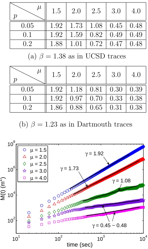
Table 3.4: Estimated MSD exponents γ using GCTRW(µ, β, p)

p

µ

1.5 2.0 2.5 3.0 4.0 0.05 1.92 1.73 1.08 0.45 0.48

0.1 1.92 1.59 0.82 0.49 0.49 0.2 1.88 1.01 0.72 0.47 0.48

(a) β = 1.38 as in UCSD traces

p

µ

1.5 2.0 2.5 3.0 4.0 0.05 1.92 1.18 0.81 0.30 0.39

0.1 1.92 0.97 0.70 0.33 0.38 0.2 1.86 0.88 0.65 0.31 0.38

(b) β = 1.23 as in Dartmouth traces

101 102 103 104

102 104 106 108

time (sec)

M(t) (m

2 )

µ = 1.5

µ = 2.0

µ = 2.5

µ = 3.0

µ = 4.0

γ = 1.92

γ = 1.73

γ = 0.45 ~ 0.48

γ = 1.08

Figure 3.7: MSD of GCTRW(µ,1.38,0.05) with µ= 1.5∼4.0

(56)

any noticeable change in the growth rate. When the step-length has infinite variance but finite mean (2 < µ < 3), γ lies between the case of finite step-length variance (µ > 3) and infinite mean step-length (µ <2). Throughout, different values ofphave little effect on γ, since the power law structure of the ‘effective’ pause time T′ (T with probability p and zero with probability 1−p) is mostly preserved. All numerical results show good match with Theorem 2.

Remark 2 While GCTRW(µ, β, p) entails power-law step-length distribution a priori, we admit the possibility that other factors such as strong correlations in angle and any

other geometrical constraints may also lead to the observed diﬀusive behavior with desired

value of γ. However, it is intractable to analytically show any relationship among those

factors and the diﬀusive behavior. In contrast, we point out that our simple model based

on generalized CTRW provides a clear-cut relationship as shown in Theorem 2 and oﬀers

an easy way to synthetically generate mobility traces with required diﬀusive behavior,

which is an essential attribute for the design and performance study of network protocols.

3.4 Numerical Results

(57)

Contact [36], Epidemic [77], Spray and Wait [73], PROPHET [54] and MaxProp [18]) by using the Opportunistic Networking Environment (ONE) simulator [41].

3.4.1 Metrics

Contact-based metrics

In the performance evaluation of DTN routing protocols, ‘contact’ is the most important factor as nodes have an opportunity of sending and receiving packets only when they are within the transmission range of other nodes. We deﬁne that there is a ‘contact’ or they ‘meet’ when two nodes are within their common transmission range r. Among many contact-related metrics [42], we distinguish between the number of new contacts and total contacts among nodes. Below are the description of contact-based metrics used in this chapter.

• The total number of new contacts: Whenever a pair of nodes meet for the ﬁrst time, this metric is incremented by one. Future contacts after the ﬁrst meeting between this pair of nodes are not counted.

• The total number of contacts: Whenever any pair of nodes meet, this metric is incremented by one.

Metric for the performance of routing protocol

Super-Diffusive Behavior in Human Mobility and Finding Relevant Models in Mobile Opportunistic Networks.

ABSTRACT

DEDICATION

To my parents

BIOGRAPHY

ACKNOWLEDGEMENTS

TABLE OF CONTENTS

LIST OF TABLES

LIST OF FIGURES

Chapter 1

Introduction

1.1

Super-diﬀusive Behavior of Mobile Nodes and

its Impact on Routing Protocols

1.2

Age Invariant Regime for Multi-Source Content

Update in Mobile Opportunistic Networks

1.3

Organization

Chapter 2

Preliminaries

2.1

Super-Diﬀusive Property

2.1.1

Mean Square Displacement (MSD)

2.1.2

Super-Diﬀusion

2.2

Content Update Scenario

2.2.1

System description

2.2.2

Content update

2.2.3

Age metric

2.3

Related Work

Chapter 3

Super-Diﬀusive Behavior of Mobile

Nodes and its Impact on Routing

Protocol Performance

3.1

Diﬀusive Behavior in GPS-based Traces and

Syn-thetic Models

3.1.1

GPS Traces Validation

time (sec)

3.1.2

Diﬀusive Behavior in Synthetic Models

3.2

Diﬀusive Behavior in AP-Based Traces

3.2.1

Available AP-Based Traces

3.2.2

MSD with Pause Time in AP-Based Traces

·

·

time (sec)

time (sec)

3.3

Continuous Time Random Walk (CTRW)

3.4

Numerical Results

3.4.1

Metrics