ABSTRACT
SAHOO, INDRANIL. Spatiotemporal Models for Physical Processes. (Under the direction of Joseph Guinness and Brian J. Reich).
With the advancement in modern technology, large-scale spatiotemporal data over regions spanning from counties to the entire globe are observed in atmospheric sciences. In this dissertation, we present a collection of models for analyzing high-dimensional spatiotemporal data on Euclidean spaces and spheres.
method of determining how well the models capture the anisotropy in the fields.
In the second part of the dissertation, we study motion winds based on space-time data collected from continual monitoring of a region or from roving monitors. These data comprise a series of images which can be used to estimate wind speed and direction at particular altitudes. In particular, the Derived Motion Winds (DMW) Algorithm esti-mates atmospheric winds by tracking features in images taken by the GOES-R series of the NOAA geostationary meteorological satellites. However, the DMW algorithm is de-terministic, and there is no way to quantify the uncertainty associated with the process. This motivates us to statistically model wind motions using a spatial process drifting in time. We consider a covariance function depending on spatial and temporal lags as well as the drift parameter, which captures the wind speed and wind direction. We estimate the parameters by maximizing the profile likelihood and smooth the estimated fields using a Gaussian kernel, weighted by the inverses of estimated variances of the estimates. Since profile likelihoods at some locations turn out to be quite flat, we consider likelihoods at neighboring locations in order to borrow strength and propose a spatially smoothed pro-file likelihood, which upon maximization should give more accurate estimates of the wind field. We conduct simulation studies to determine situations where our method should perform well. Our method has been applied to the GOES-15 brightness temperature data over Colorado and its performance has been compared to the DMW Algorithm in terms of prediction error while predicting brightness temperature fields. We also provide maps of winds over Northeast Colorado estimated using our method.
© Copyright 2018 by Indranil Sahoo
Spatiotemporal Models for Physical Processes
by Indranil Sahoo
A dissertation submitted to the Graduate Faculty of North Carolina State University
in partial fulfillment of the requirements for the Degree of
Doctor of Philosophy
Statistics
Raleigh, North Carolina
2018
APPROVED BY:
Soumendra Nath Lahiri Jacqueline Hughes-Oliver
Joseph Guinness
Co-chair of Advisory Committee
Brian J. Reich
DEDICATION
BIOGRAPHY
Indranil Sahoo was born on June 09, 1991 in Kolkata, India. He completed his secondary education (till 10th standard) in 2007 and his higher secondary education in 2009 from South Point High School, Kolkata. Having discovered an interest in Statistics during his higher secondary days, Indranil joined St. Xavier’s College, Kolkata (Autonomous) in 2009 for a Bachelor of Sciences (B.Sc.) degree in Statistics. He graduated from St. Xavier’s College in 2012 with a 1st class 1st position in B.Sc. (Statistics honors). He
ACKNOWLEDGEMENTS
This dissertation has been four years in the making; four long years rigged with hurdles and pitfalls. In these four years I have fallen down more times than I now remember. However, I have been fortunate enough to have a bunch of lovely people in my life who have always encouraged me and pushed me forward. In this section, I acknowledge their support and their contributions to my accomplishments.
First and foremost, I would like to thank my family for their constant love and support. In particular, I would like to thank my mother for her constant encouragement and my elder brother for always believing in me. When it comes to support and encouragement, the next person that comes to my mind is Shreyan. I have known him for a long time now, and I could not be more lucky to have him as my friend. He has always stood by me even through the most difficult times, and for that I thank him immensely. I would also like to thank Rahul (Saha) without whose influence I literally would not have been the person I am today.
Over the years I have had great teachers in Statistics and I am immensely grateful to each and every one of them. In particular, I would like to thank Kalyan Dey, whose enthusiasm in teaching the subject got me excited about it in the first place. I would also like to thank Professor Amit Kr. Ghosh from St. Xavier’s College, Kolkata for motivating us to go beyond the curriculum and explore the “chancy and dicey” world of Statistics.
friends like Arnab Hazra, Arkaprava, Sohini, Moumita and Arunava, and would like to thank them for being my support as I made this transition across the globe. As the years went by, Raleigh became more fun, courtesy of Pulama, Arnab Chak, Suman, Rahul, Rahul Chak, Sayak, Abhishek, Piyush, Nazmul da, Indrabati, Salil and Dhrubajyoti. I would specially like to thank Arnab Hazra and Arnab Chak for being the best roommates ever; their positivity and their willingness to help out in every situation got me through some tight situations over the past few years. A special token of love and gratitude also goes to Jim & Michele and John & Yunhee for making this city, 8664 miles away from home, home.
Even though I have been away from home for the past four years, I have remained connected to my friends back home and they too have supported me in my endeavors. I would like to thank Debanjan & Debasmita, Dipayan, Budhaditya, Abhinandan da, Chandradeep, and Shayan amongst others for their continued support and friendship.
TABLE OF CONTENTS
List of Tables . . . viii
List of Figures . . . x
Chapter 1 Introduction . . . 1
Chapter 2 A Test for Isotropy on a Sphere using Spherical Harmonic Functions . . . 5
2.1 Introduction . . . 5
2.2 Motivating Dataset . . . 9
2.3 Methodology . . . 10
2.3.1 Spherical Harmonic Representation . . . 10
2.3.2 Test Procedure . . . 13
2.4 Simulation Study . . . 15
2.4.1 Stability of the SH estimates . . . 15
2.4.2 Assessing the performance of the test . . . 19
2.5 Application to HadCM3 Model Output data . . . 25
2.6 Discussions and Conclusions . . . 31
Chapter 3 Estimating Atmospheric Wind Motions using Space-time Drift Models . . . 34
3.1 Introduction . . . 34
3.2 Derived Motion Winds Algorithm . . . 38
3.3 Space-time drift models . . . 40
3.3.1 Estimation of drift parameter . . . 42
3.3.2 Spatially-smoothed drift models . . . 44
3.4 Simulation results . . . 45
3.5 Application to GOES-15 data . . . 53
3.5.1 GOES-15 data description . . . 53
3.5.2 Estimation using GOES-15 data . . . 54
3.5.3 Comparison based on Mean Squared Prediction Error . . . 61
3.6 Discussions and Conclusions . . . 63
Chapter 4 A Graphical Model to Detect Global Teleconnections using Spherical Needlets. . . 67
4.1 Introduction . . . 67
4.2 Motivating Dataset . . . 71
4.3 Methodology . . . 71
4.3.2 Defining Teleconnections . . . 75
4.3.3 Precision Matrix Estimation . . . 77
4.4 Simulation Study . . . 79
4.5 Application to HadCM3 Model Output data . . . 81
4.6 Discussions and Conclusions . . . 87
LIST OF TABLES
Table 2.1 The maximum degree of SH that ensures computational stability during regression,lreg, and the maximum degree of SH used to
guar-antee accurate estimation of the coefficients, lcorr, for the three
dif-ferent grid sizes and the two spectra.nreg andncorr give the number
of SH functions used in each setting. lsim is chosen to be 150. . . . 18
Table 2.2 Type I error (in %) of the test for the three grid sizes, 20× 50, 73×96 and 100×200 and the two spectraCl2 and Cl3. We perform the test at 5% significance level. Here l represents the SH degrees for which we perform the test. Note that for a particular setting, we only consider l’s which are less than or equal to the corresponding
lcorr. . . 20
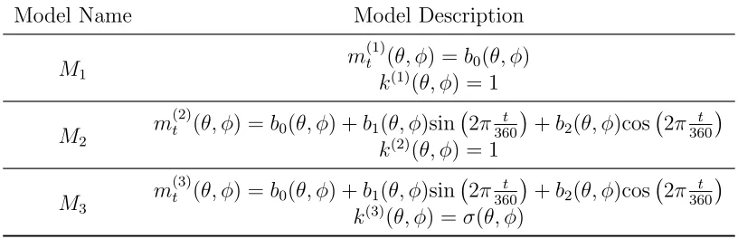
Table 2.3 Type I error (in %) of the test for the three grid sizes 20× 50, 73×96 and 100×200 and the two different spectra, Cl2 and Cl3 after accounting for temporal correlation. We perform the test at 5% significance level. . . 22 Table 2.4 Description of the three models considered. Here, b0, b1, b2 ∈R and
σ2(θ, φ) denotes the spatially varying variance. . . . 26
Table 3.1 Comparing Mean Vector Difference (SD) for Space-time Drift Model (STDM) and Derived Motion Winds algorithm (DMWA) for refer-ence wind vector (1,2)T based on data buffers of size 11×11; α2 1 and α22 denote the spatial and temporal range respectively. . . 47 Table 3.2 Comparing Mean Vector Difference (SD) for Space-time Drift Model
(STDM) and Derived Motion Winds algorithm (DMWA) for refer-ence wind vector (3,5)T based on data buffers of size 11×11; α21
and α2
2 denote the spatial and temporal range respectively. . . 47 Table 3.3 Comparing Mean Vector Difference (SD) for Space-time Drift Model
(STDM) and Derived Motion Winds algorithm (DMWA) for refer-ence wind vector (1,2)T based on data buffers of size 7×7; α2
1 and
α2
2 denote the spatial and temporal range respectively. . . 49 Table 3.4 Comparing Mean Vector Difference (SD) for Space-time Drift Model
(STDM) and Derived Motion Winds algorithm (DMWA) for refer-ence wind vector (3,5)T based on data buffers of size 7×7; α2
1 and
α22 denote the spatial and temporal range respectively. . . 49 Table 3.5 Comparing Mean Vector Difference (SD) for Space-time Drift Model
(STDM) and Derived Motion Winds algorithm (DMWA) for refer-ence wind vector (1,2)T based on data buffers of size 15×15; α21
and α2
Table 3.6 Comparing Mean Vector Difference (SD) for Space-time Drift Model (STDM) and Derived Motion Winds algorithm (DMWA) for refer-ence wind vector (3,5)T based on data buffers of size 15×15; α21
and α2
2 denote the spatial and temporal range respectively. . . 50 Table 3.7 95% coverage probabilities (in percentage) for u- and v- wind
com-ponents based on buffer size of 7× 7 and reference wind vectors (ur, vr)T = (1,2)T and (3,5)T, based on the Space-Time Drift Model
(STDM). α2
1 and α22 denote the spatial and temporal range respec-tively. . . 51 Table 3.8 95% coverage probabilities (in percentage) for u- and v- wind
com-ponents based on buffer size of 11×11 and reference wind vectors (ur, vr)T = (1,2)T and (3,5)T, based on the Space-Time Drift Model
(STDM). α12 and α22 denote the spatial and temporal range respec-tively. . . 51 Table 3.9 95% coverage probabilities (in percentages) for u- and v- wind
com-ponents based on buffer size of 15×15 and reference wind vectors (ur, vr)T = (1,2)T and (3,5)T, based on the Space-Time Drift Model
(STDM). α12 and α22 denote the spatial and temporal range respec-tively. . . 52 Table 3.10 Comparing Mean Squared Prediction Error based on prediction
us-ing the raw and smoothed wind estimates from the Space-Time Drift Model (STDM), the Spatially Smoothed Drift Model (SSDM) and the Derived Motion Winds Algorithm (DMWA) at different time points. λ in each case denotes the optimal smoothing parameter chosen using cross validation. All the methods have been compared against the baseline. . . 63
Table 4.1 Simulation results showing average numbers of estimated and non-estimated teleconnections for spatial grids of sizes 20×50 and 73×96. Herejmax has been chosen to be 2 which gives a total of 252 nodes
LIST OF FIGURES
Figure 2.1 Correlation between true and estimated coefficients for the three different grid sizes 20×50 (blue), 73×96 (red) and 100×200 (green) and for two different spectra (left versus right), as a function of the SH degreel. We consider the SH degree up to lreg in the weighted
regression. For each grid size-spectra combination, we take lcorr as
that value ofl where the corresponding correlation curve intersects the 0.999 reference line, which gives us ncorr = (lcorr + 1)2 unique
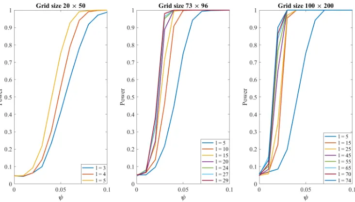
coefficients. . . 18 Figure 2.2 Empirical power functions of our test (as a function of ψ)
corre-sponding to the induced anisotropic setup for the three grid sizes and different degrees of SH,l. . . 23 Figure 2.3 Empirical power functions of our test (as a function of )
corre-sponding to the simple anisotropic scenario of different covariance structure across land and water, for the three grid sizes and differ-ent degrees of SH, l. . . 24 Figure 2.4 Pixel-wise mean air temperature (in Kelvin) based on the entire
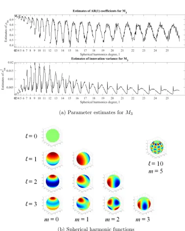
five years worth of model-output data . . . 27 Figure 2.5 (a) Estimates ofρlmandσ2lmcorresponding tom=−l, . . . ,−1,0,1, . . . , l
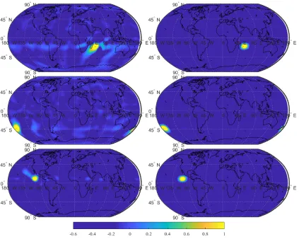
under each l for M3. (b) Spherical harmonic functions for m = 0, . . . , lforl = 0, . . . ,3. The spherical harmonics for negativemcan be depicted by rotating the positive order ones along the z-axis by 90°/m. The checkerboard pattern has been shown for l = 10, m= 5. 28 Figure 2.6 Estimates of the anisotropic (left panel) and (hypothetical) isotropic
(right panel) correlation functions at three locations around the globe, namely northeast of Mauritius (first row), around the 45°S latitude and the International Date line (second row) and North Pacific Ocean, off the coast of Mexico (third row). . . 30 Figure 3.1 Schematic of the nested tracking approach. The white vectors show
the local motion vectors successfully derived for each possible 5×5 box within a larger 15× 15 target scene. The red vector on the right is the resulting motion vector if one were to take an average of all the successfully derived local motion vectors. (Source: Daniels et al. (2010)) . . . 40 Figure 3.2 Brightness temperature maps over Colorado at 15 minutes time
Figure 3.3 Estimated standard deviations obtained using the Space-Time Drift Model (STDM), corresponding to estimated u- (left panel) and v-(right panel) components at three consecutive time points. . . 57 Figure 3.4 Raw (left panel) and smoothed (right panel) wind field estimates at
three consecutive time points obtained using the Space-Time Drift Model (STDM). . . 59 Figure 3.5 Raw (left panel) and smoothed (right panel) wind field estimates at
three consecutive time points, obtained from the Derived Motion Winds Algorithm (DMWA). . . 60 Figure 3.6 Profile loglikelihood for a particular data buffer, plotted as a
func-tion of the two components of u. . . 61 Figure 3.7 The top panel shows predicted brightness temperature fields for
three consecutive time points, obtained using smoothed wind es-timates from the Space-Time Drift Model (STDM). The second and third panels show respectively, the corresponding lower and upper prediction regions.The fourth panel shows predicted bright-ness temperature fields obtained using smoothed versions of the Derived Motion Winds Algorithm (DMWA) wind estimates. The bottom panel shows the observed temperature fields at those time points. . . 64
Figure 4.1 The average and standard deviation of critical parameters . . . . 73 Figure 4.2 Illustration of HEALPix discretization of a sphere (Gorski et al.,
2005) for j = 1. Here Nside,j = 2, which gives Nj = 48 pixels
indexed from 0 to 47. . . 75 Figure 4.3 Teleconnections observed in the North-west Pacific (top panel) and
North Atlantic-Eurasia (bottom panel) connected across frequen-cies j = 0 and j = 1 (blue: positive connection, red: negative connection). . . 83 Figure 4.4 Teleconnections observed in the Gulf of Mexico (top panel) and off
the coast of Madagascar (bottom panel) at frequency j = 2 (blue: positive connection, red: negative connection). . . 84 Figure 4.5 Teleconnection observed in the North Pacific, off the coast of
Chapter 1
Introduction
Physical processes can be defined as phenomena occurring in the Earth’s atmosphere which create constant change in features on the Earth. Studying the dynamics of physical processes and their broad environmental applications including climate, weather, and air quality have always been of interest in atmospheric sciences. It encompasses meteorology, the major focus of which is weather forecasting. Weather forecasting involves predicting the conditions of the atmosphere at a location in the future based on conditions in the past. These scenarios nicely bring into the fold statistical models and techniques, which form the basis of methodologies used to learn about uncertainties in physical processes. Nowadays, large scale climate data are collected over different regions of the globe, as well as over the entire globe. Thus is it imperative to develop statistical models to analyze space-time data over Euclidean spaces,Rd, d >1 and spheresSd−1 ={x∈Rd :kxk=r},
which is indeed the broad focus of this dissertation.
Geostatistical spatiotemporal data is often modeled using a Gaussian process model. Let {Yt(x),x ∈ D, t ∈ T } denote the physical process under consideration. Yt is said
(Yt(x1), . . . , Yt(xk)) is multivariate normal. A Gaussian process is often characterized
by its covariance function K :D × D →(0,∞) given by
K(x1,x2) = Cov (Yt(x1), Yt(x2))
The covariance function, K captures the spatial dependence among the observation and plays an important role in spatiotemporal modeling. Now, K is said to be stationary when for two locationsxi andxj,K(xi,xj) is a function of h=xi−xj, the lag between
them. Furthermore, K is said to be isotropic if it depends only onkhk.
In Chapter 3, we shift our attention to studying local winds. Winds are important for monitoring and predicting weather patterns and global climate. Winds can also affect vegetation in a region as they affect factors influencing plant growth such as seed dis-persal rates, air transportation of pollen and metabolism rates in plants. Study of local winds can give insight on power output from wind turbines, thereby helping government authorities plan and utilize winds to produce energy efficiently. It can also help gauge the intensity of calamities such as oil spills and forest fires, thereby facilitating preven-tive measures. Data on wind speed and direction are collected at ground-level weather stations on land and by buoys and ships over the ocean. Wind data can also be derived from high resolution weather data collected by geostationary satellites. These data are essentially a sequence of high resolution images collected over time. Wind speed and di-rection obtained from such satellite data play a major role in improving performance of climate models and weather forecasting. The Derived Motion Winds (DMW) Algorithm estimates atmospheric winds by tracking features in images taken by the GOES-R se-ries of the NOAA geostationary meteorological satellites. In this chapter, we discuss the shortcomings of the DMW algorithm. We propose a spatiotemporal model using a spatial process that drifts over time to analyze satellite data and obtain wind estimates. The proposed model is applied on the GOES-15 brightness temperature data over Colorado and is compared to the DMW Algorithm in terms of mean squared prediction error while predicting brightness temperature fields.
several weeks to several months, thereby adding to the variability of atmospheric pro-cesses. An example of an established teleconnection is the Southern Oscillation, which reflects periodic fluctuations in sea surface temperature and atmospheric pressure across the equatorial Pacific Ocean. Since teleconnections can influence the global climate sys-tem, it is important that we understand the abnormal behavior and interactions of these phenomena and identify them accurately. In this chapter, we propose a method for de-tecting teleconnections based on modeling spatiotemporal data using spherical needlet functions. We provide a statistical definition of a teleconnection in terms of the ‘signifi-cant’ edges in the precision matrix of the needlet coefficients. If we observe a significant edge between locations xi and xj in the same resolution, we define it to be a
telecon-nection if xi and xj do not belong to bordering needlet domain. On the other hand, if xi and xj are in different resolutions, we define the edge to be a teleconnection if the
Chapter 2
A Test for Isotropy on a Sphere
using Spherical Harmonic Functions
2.1
Introduction
Modeling spatial dependence is a major challenge when analyzing geostatistical data. It is common to assume that the spatial covariance function is isotropic, meaning that the correlation between observations at any two locations depends only on the distance between those locations and not on their relative orientation (Guan et al., 2004). With large-scale high resolution data available over the entire globe, it is important to develop methods for analyzing spatial data observed on spheres. In order to do so, it is necessary to understand the inherent correlation structure of the process on the sphere. Assuming that the process is isotropic will lead to simpler interpretation of the correlation structure and reduce computational complexity. However, in many applications, isotropy may not be a reasonable assumption and will lead to erroneous model fitting and predictions.
different directions (Cressie, 1985; Cressie and Hawkins, 1980; Cressie and Noel, 1993). Many approaches consider a stationary alternative and use directional variograms to construct test statistics (Matheron, 1962; Diggle, 1981; Caba˜na, 1987; Baczkowski and Mardia, 1990; Isaaks and Srivastava, 1989). Some nonparametric methods for checking isotropy are based on estimates of the variogram or covariogram (Lu and Zimmerman, 2001; Guan et al., 2004; Maity and Sherman, 2012). The notion of testing for second-order properties using the asymptotic joint normality of sample variogram evaluated at different spatial lags was established by Lu and Zimmerman (2001). The subsequent works of Guan et al. (2004) and Maity and Sherman (2012) are based on these ideas. Li et al. (2007, 2008); Jun and Genton (2012) consider spatiotemporal data and use approaches similar to the methods from Lu and Zimmerman (2001), Guan et al. (2004) and Maity and Sherman (2012). Bowman and Crujeiras (2013) give a more computational approach for testing isotropy in spatial data using a robust form of the empirical variogram based on a fourth-root transformation.
Haskard et al. (2007) extends the Mat´ern correlation to include anisotropy, which facilitates a test of isotropy. Fuentes (2007) describes a method in the spectral domain which is based on the estimation of parameters governing the directionality in the spatial dependence (anisotropy) using approximate likelihoods. Matsuda and Yajima (2009) once again consider a generalized Mat´ern class which allows for anisotropy and constructs a likelihood ratio test for isotropy.
All the methods discussed above are for random fields on the Euclidean space,Rd, d >
the above-mentioned tests for checking if the covariance function of the process is indeed isotropic. This necessitates the development of a test which allows us to test for isotropy on the sphere.
temporal correlation in the data while testing for spatial isotropy. We also show that the approximations employed in the test improve as the resolution of the data in space increases.
We apply the test on the near-surface air temperature projections for 2031-2035 ob-tained from the HadCM3 model. We do not expect the near-surface temperature data to be well-modeled by an isotropic model. However since we can build anisotropic models out of isotropic ones, we can apply the test on the isotropic component of anisotropic models to check anisotropic model assumptions. In this chapter, we propose a sequence of anisotropic models for our temperature data, each more complex than the previous one and each having an isotropic process as model component. We apply the proposed test on the isotropic components of the models and consider the values of the test statistic to determine how well the models capture the anisotropy in the near-surface temperature fields.
2.2
Motivating Dataset
The data set which motivated our idea is a part of the Coupled Model Intercomparison Project Phase 5 (CMIP5) archive. The CMIP 5 is a large multi-model ensemble project which has been used for the Intergovernmental Panel on Climate Change (IPCC) reports. The Hadley Centre Coupled Climate Model Version 3 (HadCM3) of the Met Office Hadley Centre (MOHC) is a coupled climate model that has been used considerably for various climate studies including climate prediction and climate modeling. HadCM3 was one of the significant models utilized as a part of the IPCC Third and Fourth Assessments, and furthermore adds to the Fifth Assessment. These models have a resolution of 2.5 degrees in latitude by 3.75 degrees in longitude, thereby producing a global grid of 73×96 grid cells. This is equivalent to a surface resolution of about 417 km ×278 km at the Equator, reducing to 295 km ×278 km at 45 degrees of latitude. These model simulations also consider a 360-day calender, where each month has 30 days.
2.3
Methodology
2.3.1
Spherical Harmonic Representation
Let Yt(θ, φ), t ∈ 1,2, . . . , T denote a Gaussian process (GP) on a sphere indexed by
latitude θ ∈ [0, π] and longitude φ ∈ [0,2π). The GP can be expressed in terms of spherical harmonic basis functions as suggested by Jones (1963). Let Sl,m(θ, φ) denote
the Schmidt semi-normalized harmonics of degree l and order m on the surface of the sphere. Analytically, Sl,m(θ, φ) can be defined as
Sl,m(θ, φ) =
q (l−m)!
(l+m)!Pl,m(cosθ)e
imφ m≥0
(−1)mS∗
l,−m(θ, φ) m <0
where * denotes complex conjugation and Pl,m(cosθ) denotes the associated Legendre
polynomial of degreel = 0,1,2, . . . and order m= 0,1, . . . , l, that is,
Pl,m(x) = (−1)m(1−x2)m/2
dm
dxmPl(x),
Pl(x) =
1 2ll!
dl
dxl(x
2−1)l.
The spherical harmonics form a complete set of orthogonal basis functions on the sphere; in particular,
Z π
θ=0 Z 2π
φ=0
Sl,m(θ, φ)Sl0,m0(θ, φ)∗sinθdφdθ =
4π
(2l+ 1)δll0δmm0
can be expressed in terms of expansions of spherical harmonic functions. Here we consider
Yt(θ, φ) = ∞
X
l=0
l
X
m=−l
almtSl,m(θ, φ) (2.1)
where {almt} is a triangular array (for each t), representing the set of complex-valued
random spherical harmonic coefficients for which the sum in (2.1) converges in mean square.
The random variables (almt)l,m are uncorrelated and form a Gaussian family if and
only if in addition to being Gaussian, Yt(θ, φ) is also isotropic (Baldi and Marinucci,
2007); also
E[Re(almt)] = 0 =E[Im (almt)], m= 0, . . . , l
and Re (almt) and Im(almt) are uncorrelated with variance
ERe(almt)2
=EIm (almt)2
=Cl/2
where Cl is the power spectrum for degree l. Thus we have Var(almt) = E
|almt|2 =
E[Re(almt)2] +E[Im(almt)2] =Cl. Since the coefficients are uncorrelated across l and
Var(Yt(θ, φ)) = ∞ X l=0 l X
m=−l
Sl,m(θ, φ)Sl,m∗ (θ, φ)Var(almt)
= ∞ X l=0 l X
m=−l
Sl,m(θ, φ)Sl,m∗ (θ, φ)Cl
= ∞ X l=0 Cl l X
m=−l
Sl,m(θ, φ)Sl,m∗ (θ, φ)
=
∞
X
l=0
Cl, by Uns¨old’s Theorem (Uns¨old, 1927).
Our testing procedure relies on a transformation from the observations Yt(θ, φ) to
the SH coefficients almt. If Yt(θ, φ) were observed continuously over the sphere, then the
spherical harmonic transform, given by
almt=
Z π
θ=0 Z 2π
φ=0
Yt(θ, φ)Sl,m(θ, φ)sinθdφdθ
can be used to recover the coefficients almt. However if we have data on a grid of size
s1×s2, we cannot recover the coefficients exactly and so we estimatealmtas the minimizer
of
s1s2
X
i=1 (
Yt(θi, φi)− lreg
X
l=0
l
X
m=−l
almtSl,m(θi, φi)
)2
4Wi (2.2)
where 4Wi is the surface area of the ith quadrangle, relative to the surface area of the
LetYtdenote the data vector for time tat all spatial locations and Y be the s1s2×T matrix [Y1, . . . ,YT]. Also let S = (Sl,m)l,m denote the matrix of the semi-normalized
harmonics, truncated at degree lreg and W denote a diagonal matrix with the weights
4Wi on the diagonal. Then minimizing the sum with respect toalmt gives the coefficient
matrix asab = (S0W S)−1S0W Y. We apply this transformation at each time point, and
use ablm• = (balm1, . . .balmT) to denote the SH coefficient corresponding to degree l and order m, replicated over time, whereas we use ab•t to denote all the coefficients at time
point t.
2.3.2
Test Procedure
Since we truncate the sum in (2.1) to represent the process, we work with a total of
nreg = (lreg + 1)2 spherical harmonics. We explore the selection of the truncation degree
lreg in Section 4 based on the stability of the regression that convertsY toab. Depending on the accuracy of the regression, we only use spherical harmonics up to degreelcorr ≤lreg
and use p = ncorr = (lcorr + 1)2 coefficients in the test. The selection of lcorr is also
described in Section 4. Since the true coefficients a are uncorrelated under isotropy, our hypotheses about isotropy are equivalent to
H0 :R=Ip versus H1 :R6=Ip
where R= Corr(a•t).
eigenvalue. Johnstone (2001) provides the distribution of the largest eigenvalue of the sample correlation matrix when sampling from a multivariate normal distribution. For this purpose, let wlm• denote the standardized SH coefficient corresponding to degree l
and order m. Notationally,
wlm• = b alm•
kbalm•k
.
Under H0, the vectors wlm• are i.i.d. Now we multiply each standardized SH coefficient
by an independent chi random variable in order to generate a standard Gaussian data matrix, denoted by ˜a(p) = (˜alm•)l,m where
˜
alm• =rlmwlm•, r2lm indep
∼ χ2T.
The test statistic is
˜
l1 =
l1( ˜C)−µT p
σT p
wherel1( ˜C) is the largest sample eigenvalue of ˜C = ˜a(p)
0
˜
a(p),µ
T p = (
√
T −1 +√p)2 and
σT p = (
√
T −1 +√p)√1 T−1 +
1
√ p
1/3
. Under the null hypothesis, when T and p both increases such that T /p→γ ≥1,
˜
l1
d
→W1 ∼F1
where F1 is the Tracy-Widom law of order 1 which is given by
F1(s) =exp
1 2
Z ∞
s
q(x) + (x−s)q2(x)dx
where q solves the nonlinear Painlev´e II differential equation
q00(x) = xq(x) + 2q3(x),
q(x)∼Ai(x) as x →+∞
and Ai(x) = 1
π
R∞ 0 cos
t3
3 +xt
dt denotes the Airy function.
The test is designed for T ≥ p but it applies equally well if T < p are both large, simply by reversing the roles of T and p in the expressions forµnp and σnp (Johnstone,
2001). The p-value for the test can be computed using the cumulative distribution table of the T W1 distribution (Bejan, 2005). Since the largest eigenvalue increases as we move away from isotropy, we have a right-tailed test.
2.4
Simulation Study
2.4.1
Stability of the SH estimates
In this section we first justify that the weighted regression technique in (2.2) gives ac-curate coefficient estimates ab when we truncate the sum in (2.1). For this purpose, we choose lsim > lreg and simulate nsim = (lsim + 1)2 Gaussian complex-valued coefficients a(nsim×T) with variance Cl, independent over T = 360 time replicates and then apply
(2.1) to get the spatial data, Yt(θ, φ) (forward transform). We evaluate how well we
re-cover a when we regress the data Y onto S, the spherical harmonics truncated at lreg
(back transform).
consider the variances
Cl =
σ2
(α2+l2)ν+1/2,
which gives rise to the Legendre-Mat´ern covariance function (Guinness and Fuentes, 2016) given by
ψ(θ) =
∞
X
l=0
σ2
(α2+l2)ν+1/2Pl(cosθ).
Hereσ2, α, ν >0 are the three parameters of the covariance function withσ2 denoting the variance, 1/αdenoting the spatial range, andν, the smoothness. The form of the Legendre Mat´ern is motivated by the Mat´ern spectral density on Rd, which is (α2+ω2)−ν−1/d. In particular, we take ν = 0.5 and ν = 1 for our simulation studies. This gives usCl of the
order of 1/l2 and 1/l3 respectively. For our convenience we refer to the two spectra as
Cl2 and Cl3 respectively. Note that the process obtained with Cl2(ν = 0.5) is not mean square differentiable. According to Hitczenko and Stein (2012) this is similar to a process with exponential covariance.
In order to ensure computational stability during regression (back transform), we choose the truncation degree of the SH, lreg, based on the condition number of S0W S,
i.e., the ratio of its smallest eigenvalue to its largest. We choose the largestlsuch that the condition number ofS0W S >0.001. The regenerated coefficients can then be expressed as
b
a•t= (S0W S)−1S0W Yt
= (S0W S)−1S0W Sa•t
since lsim > lreg.
The accuracy of the regression is summarized by the correlation between the unique real and imaginary parts of the true coefficients for each l and the corresponding esti-mates,
rl=
1 2l+ 1
l
X
m=−l
Corr(alm•,balm•)
where
Corr(alm•,almb •) =
PT
t=1(almt−¯alm)(balmt−ba
b lm)
q PT
i=1(almt−¯alm)2 q
PT
i=1(balmt−ba
b lm)2
,
¯
alm = T1
PT
t=1almtandba
b lm =
1
T
PT
t=1balmtdenote the means ofalm• andbalm• respectively. Figure 2.1 shows that the correlation between the true and estimated SH coefficients is a decreasing function of lreg. This motivates us to choose lcorr as the maximum degree of
SH for whichrl >0.999. This ensures that the weighted regression in (2.2) gives accurate
SH coefficients as long as the degree of SH considered is less than or equal to lcorr. We
also wish to study the effect of grid size on the performance of the weighted regression. With this in mind, we use three different grid sizes, namely 20×50,73×96 and 100×200 for our study. In all our numerical studies,lsim is chosen to be 150. In our data analysis,
we have a grid of size 73×96. Our numerical study indicates that under spectrumCl2 we can uselcorr up to 30, which corresponds to constructing a test on (30 + 1)2 = 961 unique
coefficients. Figure 2.1 also shows that the regression performs better with increasing grid size and also with decreasing spectra. Table 2.1 illustrates how both the number of SH used for meaningful regression and accurate estimation of the coefficients grow with l2.
(a) SpectrumCl2 (b) SpectrumCl3
Figure 2.1: Correlation between true and estimated coefficients for the three different grid sizes 20×50 (blue), 73×96 (red) and 100×200 (green) and for two different spectra (left versus right), as a function of the SH degree l. We consider the SH degree up to lreg
in the weighted regression. For each grid size-spectra combination, we take lcorr as that
value of l where the corresponding correlation curve intersects the 0.999 reference line, which gives us ncorr = (lcorr+ 1)2 unique coefficients.
Table 2.1: The maximum degree of SH that ensures computational stability during re-gression, lreg, and the maximum degree of SH used to guarantee accurate estimation of
the coefficients,lcorr, for the three different grid sizes and the two spectra. nreg and ncorr
give the number of SH functions used in each setting. lsim is chosen to be 150.
Spectrum Grid Size lreg nreg lcorr ncorr
Cl2
20×50 18 361 6 49
73×96 47 2304 30 961 100×200 85 7396 74 5625
Cl3
of the test under anisotropic models.
2.4.2
Assessing the performance of the test
Type I error under no temporal correlation
We simulate the coefficients as time-independent complex Gaussian, that is,
Re almt, Im almt ∼N(0, Cl/2), l = 1, . . . , lsim, t= 1, . . . , T = 360,
a00 ∼N(0,1.5)
withlsim = 150 and forCl2 andCl3. We follow the test procedure as described in Section 3 for the three grid sizes 20×50, 73×96 and 100×200 with appropriate choices of lreg
and lcorr as described in Table 1. We perform the test at 5% significance level. The Type
I error of the test is given by
p=P rH0(T W(T, p)> Tobs)
=P rH0
T W(T, p)−µT p
σT p
> Tobs−µT p σT p
=P rH0
T W1 >
Tobs−µT p
σT p
Table 2.2 shows the Type I error of the test for the three grid sizes and two different spectra based on 1000 simulation replications. The Type I error varies between 3% and 7% depending on the choice of l. For the recommended choice of lcorr (the final entry in
Table 2.2: Type I error (in %) of the test for the three grid sizes, 20×50, 73×96 and 100×200 and the two spectraCl2 andCl3. We perform the test at 5% significance level. Herel represents the SH degrees for which we perform the test. Note that for a particular setting, we only consider l’s which are less than or equal to the corresponding lcorr.
20×50 73×96 100×200
l Cl2 Cl3 l Cl2 Cl3 l Cl2 Cl3 3 4.3 3.4 5 4.7 5.6 5 5.3 5.3 4 5.2 3.6 10 4.8 3.7 10 5.4 5.4 5 5.0 5.3 15 5.2 3.6 15 4.9 4.9
8 4.3 20 4.7 3.7 25 3.6 3.6
10 5.2 24 4.9 5.4 35 5.0 4.8 15 5.8 27 4.8 5.6 45 4.9 4.9 29 4.7 3.7 55 5.8 5.5
35 4.5 65 4.9 4.7
40 4.3 70 4.7 4.8
45 4.4 74 5.6 5.5
47 5.2 80 4.2
Type I error under temporal correlation
Our test requires replications of the spatial process and for most applications the replications will be correlated in time. Based on our analysis of the climate temperature data in Section 2.5 and previous studies of space-time covariances (Stein, 2005) we expect the lower degree coefficients to have stronger temporal correlation than the higher degree coefficients. For our simulation study, we assume a simple AR(1) structure among the coefficients. For t = 1, . . . , T = 360,
almt =ρlalm(t−1)+elmt
where the innovations elmt are uncorrelated across l, m, and t, elmt ∼ CN(0, Cl) and
ρl = 0.9/
√
l, l= 1,2, . . . , lsim with ρ0 = 0.99, is the temporal correlation function which decays with the degree of the SH. The simulated data are transformed to real space using the forward-transform (2.1). To illustrate the importance of addressing temporal dependence in spatio-temporal data, we perform the test directly on the coefficients obtained from back-transforming the data. In such a scenario, the Type I error of the test is more than 99% for each of the grid sizes and spectra, even when the underlying spatial covariance structure is isotropic. To account for temporal dependence in our test, we treatbalm•, obtained from the back transform as a time series and estimateρl for every
(l, m) combination by regressing balm2, . . . ,balmT on balm1, . . . ,balm(T−1). We then perform the test on the innovations at 5% significance level. Table 2.3 shows the Type I error of our test once we have accounted for temporal dependence. Once again we see that the test has the right size.
Power computations
Table 2.3: Type I error (in %) of the test for the three grid sizes 20× 50, 73 ×96 and 100×200 and the two different spectra, Cl2 and Cl3 after accounting for temporal correlation. We perform the test at 5% significance level.
20×50 73×96 100×200
l Cl2 Cl3 l Cl2 Cl3 l Cl2 Cl3 3 4.7 3.7 5 4.7 4.3 5 4.7 5.3 4 4.3 4.1 10 4.6 4.5 10 4.4 5.1 5 4.4 6.0 15 4.8 4.4 15 4.8 5.1
8 5.0 20 4.9 4.8 25 4.6 5.1
10 5.2 24 5.0 5.1 35 5.2 4.9 15 5.9 27 5.3 5.0 45 4.9 5.4 29 4.5 5.4 55 4.4 5.0
35 5.7 65 4.2 4.5
40 4.3 70 4.1 4.8
45 5.7 74 4.9 5.0
47 5.3 80 4.3
85 4.3
two simple anisotropic scenarios. In the first scenario we introduce anisotropy by incorpo-rating correlation among the coefficients. In particular, we generate thealmt’s as complex
Gaussian with variance Cl2 and
Corr(almt, alm0t) =
1, m=m0
ψ, m6=m0,0≤ψ ≤1
.
Figure 2.2 plots the power by ψ for the three grid sizes 20×50, 73×96 and 100×200. All results are based on 1000 simulation replications and T = 360 independent time replications for each simulation replication. For each of the 1000 datasets we conduct the test with suitable lreg as mentioned in Table 2.2 and a few suitable l’s as listed in Table
Figure 2.2: Empirical power functions of our test (as a function of ψ) corresponding to the induced anisotropic setup for the three grid sizes and different degrees of SH, l.
Figure 2.2 shows that the test is very powerful in detecting even the slightest departures from isotropy. Even if the true correlation between two SH coefficients in the same degree is as small as 0.05, the test can almost always detect that the process has deviated from isotropy for a reasonable grid size and with a relatively small degree of the spherical harmonics. We see that the power increases with the degree of SH functions used in our analysis. The power also increases as the data points on the sphere becomes more dense. Another way to introduce anisotropy directly in the fields is to assume that the covariance structures over different parts of the globe are different. A simple way to do this is to consider different covariances over land and water. In particular, we define
gl(θ, φ) =
1, if (θ, φ)∈land
where ≥0;= 0 gives back the case of isotropy. The fields are then generated as
Yaniso;t(θ, φ) =
lsim
X
l=0
l
X
m=−l
gl(θ, φ)almtSl,m(θ, φ).
where almt, t = 1, . . . , T = 360 are simulated as complex Gaussian with variance Cl2 and independent over time. Since >0, gl(s) has the effect of reducing variance of high
frequency coefficients, resulting in smoothing processes over the ocean. Figure 2.3 plots the empirical power functions of our test as a function of with other settings the same as for Figure 2.2. Once again we consider 1000 simulations replications for estimating the power function. Once again, the test is very powerful even for very minor departures from isotropy with < 0.1. We also see that the power of the test increases with the degree of the SH used in our analysis and the grid size.
2.5
Application to HadCM3 Model Output data
We apply our method to the near-surface air temperature data obtained as an output of the HadCM3 climate model. We work with daily air temperature data from 2031 - 2035 projected on a 73×96 grid in latitude and longitude. Each month in the data has 30 days. We have 5 years worth of data with 360 time points corresponding to each year, resulting in T = 1800 time points. While we do not believe that the temperature fields are isotropic, we use the test to estimate the goodness of fit of models which seek to remove the anisotropies in the fields. We consider a few anisotropic models based on isotropic processes and we perform the test on the isotropic component of each model. In each of the models, Yt(θ, φ), t = 1, . . . , T denote the near-surface air temperature at
location (θ, φ), θ∈[0, π], φ ∈[0,2π). We consider three models of increasing complexity, and each model Mi can be written in the form
Yt(θ, φ) =m(ti)(θ, φ) +e
(i)
t (θ, φ)
1
k(i)(θ, φ)e (i)
t (θ, φ) =
X
l
X
m
almtSl,m(θ, φ)
almt =ρlmalm(t−1)+lmt
where lmt ∼N(0, σlm2 ). Table 2.4 describes the form of m
(i)
t (θ, φ) and k(i)(θ, φ) for each
of the models considered.
Table 2.4: Description of the three models considered. Here, b0, b1, b2 ∈ R and σ2(θ, φ) denotes the spatially varying variance.
Model Name Model Description
M1
m(1)t (θ, φ) =b0(θ, φ)
k(1)(θ, φ) = 1
M2
m(2)t (θ, φ) =b0(θ, φ) +b1(θ, φ)sin 2π360t +b2(θ, φ)cos 2π360t
k(2)(θ, φ) = 1
M3
m(3)t (θ, φ) =b0(θ, φ) +b1(θ, φ)sin 2π360t
+b2(θ, φ)cos 2π360t
k(3)(θ, φ) =σ(θ, φ)
results when it comes to checking if a process is indeed isotropic. Thus in each one of our models, we model the temporal dependencies in the SH coefficients as AR(1), assuming that the AR coefficients and the innovation variance vary with each (l, m) combination. For each of the models, the spatially varying mean, b0 is estimated by the pixel-wise mean temperature,
¯
Y(θ, φ) = 1 1800
1800 X
t=1
Yt(θ, φ)
which is illustrated in Figure 2.4. The other parameters inM2 and M3, namelyb1, b2, ρlm
and σ2
lm have been estimated at each pixel by regressing the lastT−1 SH coefficients on
the first T −1. We use the SH degree of l = 25 and work with (l+ 1)2 = 262 = 676 SH coefficients which means that the sample correlation matrix of the coefficients is 676×676
since the value of the test statistic for model M3 is much larger compared to a TW(1) distribution whose 99th percentile point is 2.02. The AR(1) coefficient estimates and the
estimated innovation variance corresponding to the different degrees of SH for M3 are shown in Figure 2.5.
Figure 2.4: Pixel-wise mean air temperature (in Kelvin) based on the entire five years worth of model-output data
(a) Parameter estimates for M3
(b) Spherical harmonic functions
Figure 2.5: (a) Estimates of ρlm and σlm2 corresponding to m = −l, . . . ,−1,0,1, . . . , l
pattern on the sphere untill =|m|has all the harmonics along the longitude. Figure 2.5a shows that for each degree, the m= 0 coefficient is the most correlated in time and the dependence goes down with the increase in |m|. One can say that the spectral represen-tation is analogous to the two-dimensional Fourier transform where each combination of the pair (m, n) corresponds to a two-dimensional frequency. Thus, based on Figure 2.5a we can say that the low frequency coefficients are very highly correlated compared to the high frequency ones. Figure 2.5a also shows that within each l, the temporal correlation is maximum for m = 0 and it decreases as |m| increases. Since the spherical harmonics are aligned along the latitudinal direction for m = 0 and start to get aligned along the longitudes as |m| increases, we can say that the temperature process is more correlated along the direction of the latitudes as compared to the direction of the longitudes. Figure 2.5a also shows the power spectrum of the spectral representation for ModelM3. It shows the strength of each frequency signal and tells us that lower frequencies are, in general, more important than the higher ones. In particular, the spherical harmonics between degrees 7 to 12 seem to be most meaningful in explaining the temperature process. The spectral densities for modelsM1 andM2 have dominant peaks at low frequencies, thereby overshadowing all other peaks. This is due to low frequency variation not captured by the spatially varying variance.
The innovations from M3 are still anisotropic and we point out a few locations at-tributable to the anisotropy in the process. In order to get an estimate of the anisotropic covariance of the innovation process, we use the covariance of the innovation coefficients. If ainnov denote the innovation coefficients, then the estimate of the covariance in the data illustrating the remaining anisotropy is given by Covani=SCov(ainnov)S0. On the
isotropic covariance, we shrink all the off-diagonal elements of Cov(ainnov) to zero. The
locations with large deviation between the absolute values of the estimated covariances can be thought to be the top sites contributing to the anisotropy of the near-surface air temperature fields on the Earth. Figure 2.6 shows these locations along with the anisotropic and isotropic spatial covariances.
The first location chosen is just to the north-east of the islands of R´eunion and Mauri-tius located to the east of Madagascar in the western Indian Ocean, the covariance struc-tures of which are shown in Figure 2.6, row 1. The near-surface air temperature anomalies in this region can be associated with outgoing longwave radiation (OLR) anomalies over the west Pacific Ocean (Misra, 2004). This can also be combined with the possibility that rainfall anomalies over eastern South Africa can potentially affect temperatures in the western and south-western Indian Ocean (Reason and Mulenga, 1999). Row 2 of Figure 2.6 corresponds to our second location which is in the south Pacific Ocean just above the 45°S latitude and slightly to the right of the International Date line. This can be linked to low-frequency variation in the atmospheric circulation over the Southern Hemi-sphere extratropics (Carleton, 2003). This coincides with the Southern Oscillation, which is characterized by the barometric difference between Darwin and Tahiti. Fluctuations in this difference cause temperature anomalies in parts of western Pacific and hence might lead to large anisotropies in the temperature covariance. The third location (Figure 2.6, row 3) is in the North Pacific Ocean, off the coast of Mexico. This location is at the junction of the Pacific/North American (PNA) teleconnection pattern prevalent over the central North Pacific and the equatorial Pacific Ocean which is the El Ni˜no zone. This should account for the temperature anomalies in this area which throws the covariance structure in the temperature fields away from isotropy.
2.6
Discussions and Conclusions
structure on the globe is isotropic. However in most real-life applications, this assumption does not hold. In this chapter, we have proposed a method to determine the aptness of this simplifying assumption.
We assume that a particular meteorological variable is distributed as a GP on a sphere and we express the process as a linear combination of the spherical harmonic functions which form a complete set of orthogonal basis functions on the sphere. Under the further assumption of isotropy, the spherical harmonic coefficients are uncorrelated, Gaussian (Baldi and Marinucci, 2007). We use this characterization to set up a test for isotropy based on the sample correlation among the coefficients. The test statistic, based on Johnstone (2001) is given in Section 2.3.2. We provide conditions to ensure computational stability and accuracy during regression in Section 2.4.1.
We show how the test is sensitive to temporal correlation, and we have provided a modeling framework for addressing temporal correlation that gives accurate Type I error rates. This has been demonstrated in Section 2.4.2 where we consider a decaying temporal correlation among the coefficients and perform the test before and after modeling the temporal dependencies. It must be very evident that most spatio-temporal processes are not isotropic and our method provides a way to objectively perform a test to help arrive at that conclusion. Also one can easily arrive at possible locations in the data attributing to anisotropy using our method. As seen in our data analysis, even for the most complex model considered, the test for isotropy gets rejected. This highlights the need for developing better anisotropic models which will better capture the global anisotropic covariance structures of spatiotemporal processes.
Acknowledgements
Chapter 3
Estimating Atmospheric Wind
Motions using Space-time Drift
Models
3.1
Introduction
prediction of propagation of oil-spills (Kim et al., 2014) and the study of coastal ero-sion (Ahmad et al., 2015). Local winds are also capable of moving pollutants into an area (for example, Calima, which blows dust into the Canary Islands; source: https:
//www.weatheronline.co.uk/reports/wind/The-Calima.htm) and may impact large-scale devastations such as forest fires (for example, the Santa Ana winds, which blows into California after the scorching summers; source:https://www.washingtonpost.com/
graphics/2017/national/santa-ana-fires/). Thus it is important to build spatio-temporal models to get ideas about the strength and direction of local winds to help us prepare for natural calamities and facilitate preventive measures.
approach to describe the space-time dependencies of the data.
On the other hand, geostationary weather satellites provide data from the surface and the atmosphere with a very high temporal resolution. The resulting data comprise a series of images which essentially make them a ‘movie’. These satellite image sequences can be used to derive wind estimates over a certain region by tracking movements of atmospheric tracers such as clouds or moisture features over time. Wind data thus ob-tained by satellites play a major role in data assimilation. Numerical climate models perform better with an increased wind data, especially over the oceans. In this way satel-lite derived winds improve weather forecasts and warnings. The European Centre for Medium-Range Weather Forecasts (ECMWF) has been implementing atmospheric mo-tion winds into their forecast models operamo-tionally since the 1980s. This has dramatically improved the model’s ability to forecast the track of tropical cyclones and has also in-creased the model’s ability to predict wave heights and storm surges (Tomassini et al., 1999).
Note that the DMW algorithm is completely deterministic; it does not take into account the issues that might lead to uncertainty in the measurements reported by the satellites. In particular, quantifying uncertainties using the SSD criterion is hard because each es-timated vector uses a different subset of the data and so likelihood ratio tests are not applicable. Also the vector estimates generated can at most be half-integers.
To overcome these shortcomings, appropriate statistical methods are necessary to es-timate wind motion over time. This motivates us to model satellite image data using a spatial process drifting in time. At the heart of this statistical model lies the idea of incorporating the motion vector parameters in the process covariance. We borrow the idea of Nested Tracking from Daniels et al. (2010) by considering data buffers and us-ing a slidus-ing window over space and estimate the local wind speed and direction usus-ing maximum likelihood estimates. Local estimation of covariance parameters using moving windows has been studied in Haas (1990, 1995). One major advantage of our approach over the DMW algorithm is that it allows us to quantify uncertainties associated with the estimates in terms of their estimated variances. The estimated wind fields are smoothed using weighted Gaussian kernels, the weights being equal to the estimated inverse vari-ances of the estimates. This ensures that our estimated drift vectors can be any real vector. This not only enables us to make smooth maps of wind over specific regions but also permits us to quantify the uncertainty associated with the estimated wind fields.
algorithm based on prediction accuracy. We also include maps of estimated motion winds over Northeast Colorado. Some concluding remarks are given in Section 3.6.
3.2
Derived Motion Winds Algorithm
The Derived Motion Winds (DMW) Algorithm is an algorithm for estimating atmospheric motion winds from images taken by the Advanced Baseline Imager (ABI) flown on the Geostationary Operational Environmental Satellite Series R (GOES-R) series of the Na-tional Oceanic and Atmospheric Administration (NOAA) geostationary meteorological satellites. If the satellite is tracking a cloudy region, the imager records the brightness temperature, which measures the radiance of the microwave radiation traveling upward from the top of the atmosphere to the satellite (expressed in Kelvin scale). For clear sky portions, the satellite records images of suitable indicators of atmospheric moisture content, such as specific humidity. Here, a ‘target scene’ is represented by a square array of pixels defining a suitable feature whose movement can be tracked in time. The size of this array depends on the spatial and temporal resolution of the imagery and the scale of the intended feature to be tracked. Daniels et al. (2010) provides a description of and the physical basis for the estimation of atmospheric winds from the images taken by the GOES-R satellite.
computed. The mean displacement vector is computed from the two displacements and is assigned to time t0 as the final DMW. Here ∆tdenotes the temporal resolution of the images. It has been suggested that the temporal resolution of the images should at most be 15 minutes in order to account for the short lifespan and rapid disintegration of clouds over land. Daniels et al. (2010) also gives a description of the Nested Tracking Algorithm which can capture the local wind motions and addresses the fact that averaging conflicting motions within the target scene can result in erroneous estimates. This algorithm involves nesting smaller target scenes (usually of size 5×5) within a larger target scene of size 15×15 and getting every possible local motion vectors derived from each possible smaller
box within a larger target scene. This is done by tracking the smaller target scene back and forward in time within a larger search region around it. The corresponding displacement vectors are computed by minimizing the Sum of Squared Differences (SSD) criteria
SSD(dx1, dx2) =
X
x1
X
x2
{I1(x1, x2)−I2(x1+dx1, x2+dx2)}
2
with respect to (dx1, dx2), whereI1 denotes the response within the smaller box, centered
at pixel locationx= (x1, x2)T,I2denotes the response within the displaced box, centered at pixel location (x1+dx1, x2+dx2) of the search window and the sum is considered over
two dimensions. In practice, the region over which the search is conducted is substantially larger than the size of the smaller target scene, so the above summation is carried out for all target box positions within the search region. The mean displacement vector is com-puted from the two displacements and is assigned as the final DMW estimate at location
displace-Figure 3.1: Schematic of the nested tracking approach. The white vectors show the local motion vectors successfully derived for each possible 5×5 box within a larger 15×15 target scene. The red vector on the right is the resulting motion vector if one were to take an average of all the successfully derived local motion vectors. (Source: Daniels et al. (2010))
ments belonging to the largest cluster. Figure 3.1 illustrates the schematics of the Nested Tracking Algorithm.
3.3
Space-time drift models
LetY(x, t) denote the brightness temperature at locationxand timet. We modelY(x, t) as
Y(x, t) = µ(x, t) +Z(x, t) (3.1)
in terms of the spatial and temporal lags. However, the concept of space-time isotropy is not so relevant because it does not make sense to treat time as another spatial dimension as time has different units. So it is logical to assign a different range parameter to time. Another common feature in space-time processes is the lack of full symmetry in the covariance structure. By this we mean
K{(x, t1),(y, t2)} 6=K{(x, t2),(y, t1)} (3.2)
for all x,y, t1 and t2, where K{(x, t1),(y, t2)} denotes the covariance function of the process Z(x, t) at (x, t1) and (y, t2). In most regions, winds tend to flow in a consistent direction, and so changes in temperature or precipitation rate at one location tend to pre-cede similar changes at another location in the direction of the flow. For instance, ift2 > t1 and winds flow consistently from xto y, then K{(x, t1),(y, t2)}> K{(x, t2),(y, t1)}.
Here we modelZ(x, t) from (3.1) using a process that drifts over time. SupposeZ0 is a stationary, space-time symmetric process with covariance function C0. ThenZ(x, t) is defined as
Z(x, t) =Z0(x−u(x, t)t, t)
where the drift parameter u(x, t) is a two-dimensional vector denoting the orthogonal components of the wind vector at location x and time point t. The covariance function of Z(x, t) is given by
K{(x, t1),(y, t2)}= Cov{Z(x, t1), Z(y, t2)}
= Cov{Z0(x−u(x, t1)t1, t1), Z0(y−u(y, t2)t2, t2)}
=σ2C0{x−y− {u(x, t1)t1−u(y, t2)t2}, t1−t2}
Let us assume that the winds are constant and move linearly in space and time. Then, the covariance function of Z(x, t) is
K{(x, t1),(y, t2)}=σ2C0{x−y−u(x, t)(t1−t2), t1−t2}
=σ2C0
s
kd−u(x, t)hk2
α2 1
+ |h| 2
α2 2
(3.4)
where d = x− y denotes the spatial lag, h = t2 − t1 denotes the temporal lag and
C0 is taken to be the standard exponential covariance function. Also, α21 and α22 denote respectively the spatial and temporal range parameters and σ2 is the variance. Note that, the process covariance has been expressed through deformations of the geographic coordinates. According to Sampson and Guttorp (1992),K is a valid covariance function of a spatiotemporal process if and only if K is a function of the Euclidean distances between site locations, which are bijection to the geographic coordinate system. That is, for K to be a valid covariance function, x−u(x, t)t needs to be bijection tox. Fuentes et al. (2008) model a drift process using a Bayesian analysis of a global model as described above. In particular, the drift parameter is modeled using splines. However this approach will be very slow for our problem and hence our proposed model should be favored.
3.3.1
Estimation of drift parameter
We first standardize the data to remove the spatially varying mean and variance. Let
Z(x, t) = Y(x, t)−bµ(x) b
σ(x)
re-maining correlation parameters to be estimated. In order to estimate the wind motions locally, we define a data buffer as
D(x, t) = {(s, t0) such that kx−sk< &|t−t0| ≤1}.
We assume that the process Y(x, t) is stationary in D(x, t). Within the data buffer considered, we use maximum likelihood estimation to estimate θ(x, t)≡θD. That is, for
a fixed data buffer D at location x and time t, if ZD(n×1) denotes the standardized
data vector in the buffer and ΣθD(n×n) denote the corresponding space-time covariance
matrix, then the log-likelihood for (σ2
D,θD) given ZD is given by
l θD, σD2|ZD
=−n
2log(2π)− 1 2log |σ
2
DΣθD|
− 1 2σ2
D
[ZD −1βD]T Σ−θD1[ZD −1βD] (3.5)
whereµD =1βD andσD2 are the local mean and variance of the data in D. For fixedθD,
the maximum likelihoods of βD and σ2D are given by
b
βD,θD = 1
TΣ−1 θD1
−1
1TΣ−θ1
DZD
b
σ2
b βD,θD =
1
n
ZD−1βbD,θD T
Σ−θ1
D
ZD−1βbD,θD
Plugging in the above estimates of βD and σD2 in 3.5, we get the profile log-likelihood for θD,
pl(θD|ZD) =−
1 2
nlogbσ2
b βD,θD
+ log(|ΣθD|)
We now maximize this profile log-likelihood to get the maximum likelihood estimate of
θD. We also estimate the variances associated with the estimated wind fields by
comput-ing the observed inverse hessian matrix at the maximum likelihood estimate, θbD. The estimates obtained are associated with the location xand time pointt at which the data buffer D was centered. We imitate the Nested Tracking approach and slide the buffer window across space and time, and estimate the wind vectors locally.
3.3.2
Spatially-smoothed drift models
The profile log-likelihood in 3.6 for a particular data buffer over a grid ofu is often very flat (see Figure 3.6). We believe that flat profile log-likelihoods make the optimization in our method harder, which in turn lead to estimates with high variances.
Therefore, we propose the idea of spatially smoothing out the profile likelihood corre-sponding to bufferD(s, t), so that the likelihood forDborrows strength from neighboring data buffers. We use a scaled version of the Gaussian kernel
φ(s|xl, λ) =
1 2πλ2exp
−||s−xl|| 2
2λ2
,
where λ > 0 is the kernel bandwidth, s denotes the center of D and x1, . . . ,xk ∈ R2
denote the centers of k neighboring data buffers. The smoothing weights are defined as
wl(s) =
φ(s|xl, λ)
Pk
j=1φ(s|xj, λ)
. (3.7)
Herewl(s) ensures that the weights at each neighboring location sum to 1. IfZD denotes
given by
pl(s)(θD|ZD,Z(xi, t)) = k
X
i=0
pl (θD|Z(xi, t))wl(s) (3.8)
where x0 = s. We call this approach, the spatially smoothed drift model (SSDM). We maximize the SSDM profile log-likelihood to get estimates of the local wind fields,
b
θD;SSDM.
3.4
Simulation results
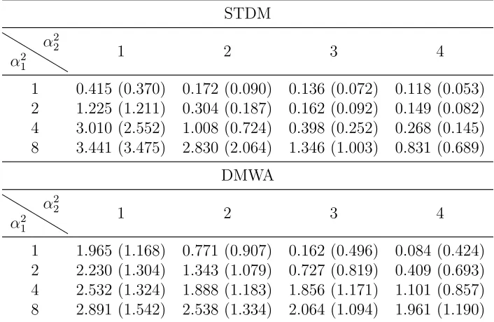
This section details some simulations performed in order to determine the conditions under which the space-time drift model (STDM) performs well while estimating wind motion vectors. We also implement a version of the DMW algorithm under similar con-ditions and compare its performance with the STDM. To compare the two methods, we compute the accuracy and precision estimates described in Daniels et al. (2010). Accuracy is measured by the Mean Vector Difference (MVD)
V Di =
q
(ubi−ur)2+ (bvi−vr) 2
, M V D= 1
N
N
X
i=1
V Di
where (ubi,bvi) denotes the estimated wind vector for the i
th simulated data buffer and
(ur, vr) denotes the reference (‘true’) wind. The standard deviation about the MVD,
SD = v u u t 1
N −1
N
X
i=1
(V Di−M V D)2
measures the precision.
to be either 1, 2, 4 or 8, and the true temporal range parameter α2
2 is chosen to be either 1, 2, 3 or 4. We also take two different values of the reference wind vector, namely (ur, vr)T = (1,2)T and (3,5)T which signify respectively slow and fast wind vectors.
All four parameters are updated simultaneously during optimization. Tables 3.1 and 3.2 compare the performance of the two methods for the two wind vectors based onN = 100 simulations.
Table 3.1: Comparing Mean Vector Difference (SD) for Space-time Drift Model (STDM) and Derived Motion Winds algorithm (DMWA) for reference wind vector (1,2)T based on
data buffers of size 11×11; α2
1 andα22 denote the spatial and temporal range respectively. STDM
α21 α22
1 2 3 4
1 0.415 (0.370) 0.172 (0.090) 0.136 (0.072) 0.118 (0.053) 2 1.225 (1.211) 0.304 (0.187) 0.162 (0.092) 0.149 (0.082) 4 3.010 (2.552) 1.008 (0.724) 0.398 (0.252) 0.268 (0.145) 8 3.441 (3.475) 2.830 (2.064) 1.346 (1.003) 0.831 (0.689)
DMWA
α2 1
α2
2 1 2 3 4
1 1.965 (1.168) 0.771 (0.907) 0.162 (0.496) 0.084 (0.424) 2 2.230 (1.304) 1.343 (1.079) 0.727 (0.819) 0.409 (0.693) 4 2.532 (1.324) 1.888 (1.183) 1.856 (1.171) 1.101 (0.857) 8 2.891 (1.542) 2.538 (1.334) 2.064 (1.094) 1.961 (1.190)
Table 3.2: Comparing Mean Vector Difference (SD) for Space-time Drift Model (STDM) and Derived Motion Winds algorithm (DMWA) for reference wind vector (3,5)T based on
data buffers of size 11×11; α2
1 andα22 denote the spatial and temporal range respectively. STDM
α21 α22
1 2 3 4
1 1.124 (1.089) 0.868 (1.503) 0.743 (1.573) 0.530 (1.062) 2 1.916 (1.685) 0.777 (1.236) 0.299 (0.415) 0.230 (0.409) 4 2.820 (1.981) 1.489 (1.358) 0.676 (0.699) 0.392 (0.365) 8 3.401 (2.842) 3.125 (1.959) 2.071 (1.803) 1.129 (1.027)
DMWA
α2 1
α2
2 1 2 3 4