ABSTRACT
MA, YANTING. Solving Large-Scale Inverse Problems via Approximate Message Passing and Optimization. (Under the direction of Dror Baron.)
This work studies the problem of reconstructing a signal from measurements obtained by a sensing system, where the measurement model that characterizes the sensing system may be linear or nonlinear.
We first consider linear measurement models. In particular, we study the popular low-complexity iterative linear inverse algorithm, approximate message passing (AMP), in a prob-abilistic setting, meaning that the signal is assumed to be generated from some probability distribution, though the distribution may be unknown to the algorithm. The existing rigorous performance analysis of AMP only allows using a separable orblock-wise separable estimation function at each iteration of AMP, and therefore cannot capture sophisticated dependency structures in the signal. This work studies the case when the signal has a Markov random field (MRF) prior, which is commonly used in image applications. We provide rigorous performance analysis of AMP with a class of non-separable sliding-window estimation functions, which is suitable to capture local dependencies in an MRF prior.
In addition, we design AMP-based algorithms with non-separable estimation functions for hyperspectral imaging and universal compressed sensing (imaging), and compare our algorithms to state-of-the-art algorithms with extensive numerical examples. For fast computation in large-scale problems, we study a multiprocessor implementation of AMP and provide its performance analysis. Additionally, we propose a two-part reconstruction scheme where Part 1 detects zero-valued entries in the signal using a simple and fast algorithm, and Part 2 solves for the remaining entries using a high-fidelity algorithm. Such two-part scheme naturally leads to a trade-off analysis of speed and reconstruction quality.
Solving Large-Scale Inverse Problems via Approximate Message Passing and Optimization
by Yanting Ma
A dissertation submitted to the Graduate Faculty of North Carolina State University
in partial fulfillment of the requirements for the Degree of
Doctor of Philosophy
Electrical Engineering
Raleigh, North Carolina 2017
APPROVED BY:
Jack Silverstein Minor Member
Brian Hughes
Cranos Williams Deanna Needell
External Member
Ahmad Beirami External Member
Dror Baron
BIOGRAPHY
Yanting Ma received the B.S. degree in communication engineering from Wuhan University, China and started the graduate program at the Department of Electrical and Computer En-gineering of North Carolina State University in 2012. She was a research intern at Mitsubishi Electric Research Laboratories (MERL), Cambridge, MA, in the summers of 2016 and 2017.
ACKNOWLEDGMENTS
I would like to first thank my advisor Prof. Dror Baron for providing me with the opportunity to pursue research topics that I am truly enthusiastic about. I especially thank him for helping me build connections to the great people whom I would like to thank in the following.
My deepest thanks go to Prof. Min Kang. From the two probability courses that I took with her, I started to appreciate the beauty of math. Building the good habit of learning rigorously and understanding materials thoroughly has been extremely helpful in my later studies. I also thank Prof. Kang for her kindness and encouragement during hard times.
Thanks to Prof. Jack Silverstein for being on my committee and for, together with Prof. Kang, helping me learn convex analysis in a completely rigorous way. Our study on convex optimization created the opportunity for my second internship at Mitsubishi Electric Research Laboratories (MERL). Without their help in improving my mathematical skills, I would not be confident in pursuing the interesting research topics in the later stage of my PhD journey.
Thanks also to my other primary collaborators: Prof. Cynthia Rush, Prof. Ulugbek Kamilov, Prof. Yue Lu, Prof. Deanna Needell, Dr. Ahmad Beirami, Dr. Jin Tan, and Dr. Junan Zhu. I would especially thank Cindy for working closely with me on state evolution analysis of approximate message passing, which is presented in Chapter 2 and Appendix A. (You may notice that this work occupies almost half of this dissertation.) Ulugbek opened the door to the fascinating field of computational imaging for me and our work is presented in Chapter 5 and Appendix D. I thank Ulugbek for hosting me at MERL and sharing his creative ideas. Thanks to Jin for her help with my research in the early stage of the program and being a considerate friend. What I gained from my collaborators is much more than just publications, of course. Their way of thinking and approaching problems would definitely influence me in the future.
I thank Prof. Cranos Williams and Prof. Brian Hughes for being on my committee and pro-viding valuable comments. Thanks to my other collaborators at MERL, Dr. Petros Boufounos, Dr. Dehong Liu, Dr. Hassan Mansour, Dr. Yuichi Taguchi, and Dr. Anthony Vetro. The two summer internships at MERL were invaluable experiences for me. There I found an open-minded research culture and exciting multidisciplinary research topics. Also from MERL, thanks to Dr. Teng-Yok Lee and Dr. Chungwei Lin for insightful discussions and for being good friends.
Thanks to Prof. Ramji Venkataramanan for his generous help with my application for the Newton International Fellowships, where he devoted a large amount of time discussing re-search directions with me and revising my rere-search proposal. Although the application was not awarded, I wish to collaborate with Ramji and pursue the proposed research in the future. Also for this application, I thank Prof. Daniel Stancil, Prof. Wei Dai, Prof. Yue Lu, and Prof. Dror Baron for writing reference letters for me.
TABLE OF CONTENTS
LIST OF FIGURES . . . vi
Chapter 1 Introduction . . . 1
1.1 Approximate Message Passing for Linear Inverse Problems . . . 2
1.2 Nonlinear Diffractive Imaging via Optimization . . . 3
1.3 Dissertation Organization . . . 3
1.4 Notation . . . 4
Chapter 2 State Evolution Analysis of Approximate Message Passing with Non-Separable Denoisers . . . 5
2.1 Definition of the Algorithm . . . 6
2.2 Performance Analysis . . . 10
2.2.1 Definitions and Assumptions . . . 10
2.2.2 Main Result . . . 12
2.2.3 Numerical Examples . . . 15
2.3 Proof of Theorem 2.2.1 . . . 18
2.3.1 Proof Notation . . . 19
2.3.2 Concentrating Constants . . . 21
2.3.3 Conditional Distribution Lemma . . . 23
2.3.4 Main Concentration Lemma . . . 26
2.3.5 Proof of Theorem 2.2.1 . . . 28
2.4 Proof of Lemma 2.3.4 . . . 29
2.4.1 Step 2: Showing thatH1 holds . . . 29
2.4.2 Step 4: Showing thatHt+1 holds . . . 34
2.5 Additional Result for 1D Signals with Markov Chain Priors . . . 39
2.5.1 Definitions and Assumptions . . . 39
2.5.2 Performance Guarantee . . . 40
2.5.3 Proof of Theorem 2.5.1 . . . 41
2.6 Conclusion . . . 46
Chapter 3 Application of Approximate Message Passing with Non-Separable Denoisers . . . 48
3.1 Approximate Message Passing with Universal Denoiser . . . 49
3.1.1 Related Work . . . 49
3.1.2 Proposed Method . . . 51
3.1.3 Numerical Results . . . 58
3.2 Approximate Message Passing with Adaptive Wiener Filter . . . 64
3.2.1 Problem Formulation . . . 64
3.2.2 Proposed Method . . . 65
3.2.3 Numerical Results . . . 66
3.3 Conclusion . . . 67
4.1 Multiprocessor Approximate Message Passing with Column-Wise Partitioning . . 70
4.1.1 Definition of the Algorithm . . . 71
4.1.2 Performance Analysis . . . 72
4.1.3 Proof of Theorem 4.1.1 . . . 74
4.1.4 Numerical Examples . . . 79
4.2 Two-Part Reconstruction Framework . . . 81
4.2.1 The Noisy-Sudocodes Algorithm . . . 81
4.2.2 Performance Analysis . . . 83
4.2.3 Trade-Off between Runtime and Reconstruction Quality . . . 89
4.2.4 Application to 1-Bit Compressed Sensing . . . 91
4.3 Conclusion . . . 95
Chapter 5 Nonlinear Diffractive Imaging via Optimization . . . 96
5.1 Related Work . . . 96
5.2 Problem Formulation . . . 97
5.2.1 Scalar Field Setting . . . 97
5.2.2 Vectorial Field Setting . . . 99
5.2.3 Nonconvex Optimization Formulation . . . 102
5.3 Proposed Method . . . 103
5.4 Experimental Results . . . 106
5.5 Conclusion . . . 108
Chapter 6 Discussion . . . .112
BIBLIOGRAPHY . . . .115
APPENDICES . . . .126
Appendix A Chapter 2 Appendix . . . 127
A.1 Concentration Lemmas . . . 127
A.2 Other Useful Lemmas . . . 128
A.3 Concentration with Dependencies for Theorem 2.2.1 . . . 129
A.4 Concentration with Dependencies for Theorem 2.5.1 . . . 136
Appendix B Chapter 3 Appendix . . . 151
B.1 Derivation of (3.4) . . . 151
Appendix C Chapter 4 Appendix . . . 154
C.1 Proof of Lemma 4.1.2 . . . 154
C.2 Proof of Lemma 4.2.1 . . . 156
C.3 Proof of Lemma 4.2.2 . . . 158
Appendix D Chapter 5 Appendix . . . 159
D.1 Proof of Proposition 5.3.1 . . . 159
D.2 Proof of Proposition 5.3.1 . . . 160
D.3 Convergence Analysis . . . 161
D.3.1 Definitions and Standard Results . . . 161
LIST OF FIGURES
Figure 2.1 For Λ of size 3×3, the denoiser ηt:RΛ→Rmay only process the pixels in gray (the center and the four adjacent pixels). . . 8 Figure 2.2 Illustration of the definition of “missing” entries in a sliding window inZ2.
The matrix v∈R4×4. The half-window size isk = 1, thus Λ = [3]×[3]. For the window Λ(1,1) centered at coordinate (1,1), the “existing” entries in the window are v1,1, v1,2, v2,1, v2,2 as shown in dark gray. Five entries, which are in light gray, are missing, hence we define their value to be the average of the existing ones, ¯v= 14(v1,1+v1,2+v2,1+v2,2). . . 9 Figure 2.3 Numerical example. From left to right: ground-truth image generated by
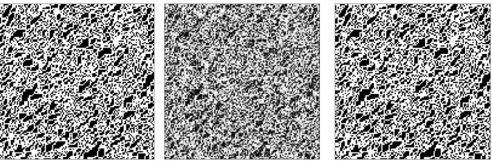
the MRF described in Section 2.2.3.1, image reconstructed by AMP with a separable Bayesian denoiser (computed from the incorrect assumption that the signal is generated from an i.i.d. Bernoulli distribution), and image reconstructed by AMP with a Bayesian sliding-window denoiser with k= 1, hence Λ = [3]×[3]. (Γ = [128]×[128], δ= 0.5, SNR = 17 dB.) 16 Figure 2.4 Numerical verification that the empirical MSE achieved by AMP with
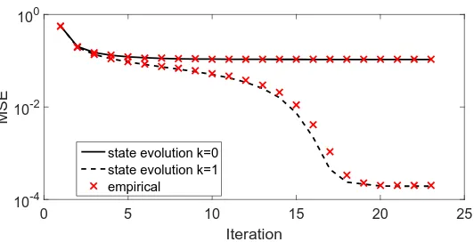
sliding-window denoisers is tracked by state evolution. The empirical MSE is averaged over 50 realizations of the MRF (as described in Section 2.2.3.1), measurement matrix, and measurement noise. (Γ = [128]×[128],
δ = 0.5, SNR = 17 dB.) . . . 17 Figure 2.5 Reconstruction of texture images using AMP with different denoisers.
From left to right: original gray level images, binary ground-truth images, images reconstructed by AMP with a total variation denoiser [8], non-separable Bayesian sliding-window denoiser (MRF prior, k = 1), and separable Bayesian denoiser (Bernoulli prior), respectively. From top to bottom: images of cloud, leaf, and wood, respectively. (Γ = [128]×[128],
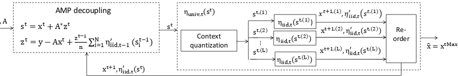
δ = 0.3, SNR = 20 dB.) . . . 18 Figure 3.1 Flow chart of AMP-UD. AMP decouples the linear inverse problem into
denoising problems. In the tth iteration, the universal denoiser ηuniv,t(·) converts stationary ergodic signal denoising into i.i.d. signal denoising. Each i.i.d. denoiser ηiid,t(st,(l)) generates the denoised signal xt+1,(l) and the derivative of the denoiser η0iid,t(st,(l)) forl∈[L]. The algorithm stops when the iteration index t reaches the predefined maximum tMax, and outputs bxtMax as the final result. . . 52 Figure 3.2 Comparison of the reconstruction results obtained by the two AMP-UD
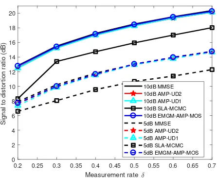
implementations to those by SLA-MCMC and EM-GM-AMP-MOS for simulated i.i.d. sparse Laplace signals. Note that the SDR curves for the two AMP-UD implementations and EM-GM-AMP-MOS overlap the MMSE. . . 60 Figure 3.3 Comparison of the reconstruction results obtained by the two AMP-UD
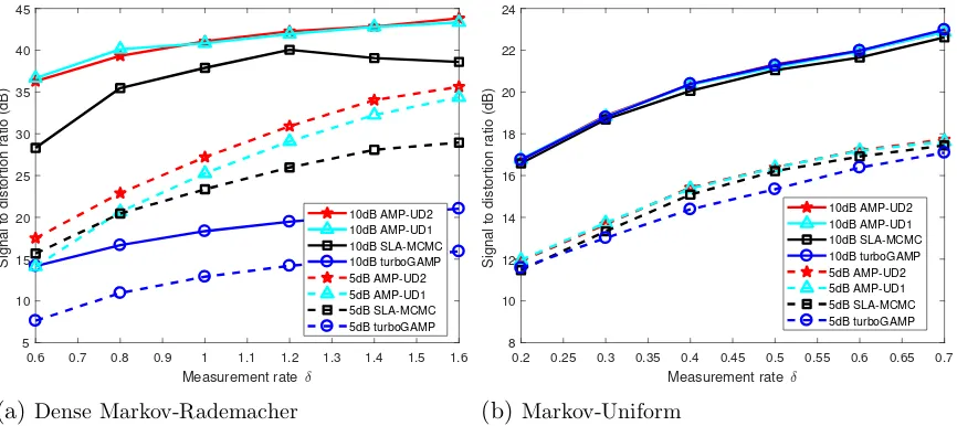
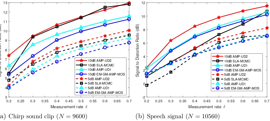
Figure 3.4 Comparison of the reconstruction results obtained by the two AMP-UD implementations to those by SLA-MCMC and EM-GM-AMP-MOS for real-world signals. . . 62 Figure 3.5 Comparison of the reconstruction results obtained by AMP-UD2 to those
by AMP-BM3D for images of size 128×128 from noiseless measurements. From top to bottom: ground-truth images, images reconstructed by AMP-UD2, and images reconstructed by AMP-BM3D. From left to right: the first four columns are natural images (δ = 0.3), and the last column is a realization of the MRF defined in Section 2.2.3.1 (δ = 0.5). . . 63 Figure 3.6 The matrix H is presented for K = 2, I = J = 8, and L = 4. The
circled diagonal patterns that repeat horizontally correspond to the coded aperture pattern used in the first FPA shot. The second coded aperture pattern determines the next set of diagonals. . . 65 Figure 3.7 The Lego scene. (The target object presented in the experimental results was
not endorsed by the trademark owners and it is used here as fair use to illus-trate the quality of reconstruction of compressive spectral image measurements. LEGO is a trademark of the LEGO Group, which does not sponsor, authorize or endorse the images in this work. The LEGO Group. All Rights Reserved. http://aboutus.lego.com/en-us/legal-notice/fair-play/.) . . . 67 Figure 3.8 Comparison of AMP-3D-Wiener, GPSR, and TwIST for the Lego image
cube. Cube size is I = J = 256, and L = 24. The measurements are captured withK = 2 shots using complementary random coded apertures, and the number of measurements isn= 143,872. Random Gaussian noise is added to the measurements such that the SNR is 20 dB. . . 68 Figure 4.1 C-MP-AMP for Gaussian matrices. . . 80 Figure 4.2 C-MP-AMP for non-Gaussian matrices. . . 81 Figure 4.3 Top: Relative error between the empirical and theoretical probability of
missed detection. Bottom: Relative error between the empirical and the-oretical probability of false alarm. (The thethe-oretical probabilities rely on the asymptotic independence result of Lemma 4.2.1.) . . . 86 Figure 4.4 Numerical verification of approximations made in the analysis of Part 2. . 89 Figure 4.5 Trade-offs between reconstruction quality, measurement rate δ, and
run-time of Noisy-Sudocodes with AMP in Part 2. . . 90 Figure 4.6 Numerical verification of the prediction for SDR (3.10) (top) and runtime
(bottom) of Noisy-Sudocodes with AMP in Part 2. . . 91 Figure 4.7 Numerical results of Noisy-Sudocodes with BIHT in Part 2 in a noisy
1-bit CS setting. In both figures, Top: SDR as a function of measurement rate δ. Bottom: SDR as a function of runtime. (n1/N = 0.1,n2=n−n1,
Figure 5.1 Visual representation of the measurement scenario considered in this work. An object with a real permittivity contrastχ(r) is illuminated with an input wave uin(r), which interacts with the object and results in the scattered wave usc at the sensor domain Γ⊂R2. The complex scattered wave is captured at the sensor and the algorithm proposed here is used for estimating the contrast χ. . . 98 Figure 5.2 The measurement scenario for the 3D case considered in this work. The
object is placed within a bounded image domain Ω. The transmitter an-tennas (Tx) are placed on a sphere and are linearly polarized. The arrows in the figure define the polarization direction. The receiver antennas (Rx) are placed in the sensor domain Γ within the x-y (azimuth) plane, and are linearly polarized along the z direction. . . 99 Figure 5.3 Empirical convergence speed for relaxed FISTA with various α values
tested on experimentally measured data. . . 105 Figure 5.4 Comparison of different reconstruction methods for various contrast levels
tested on simulated data. . . 107 Figure 5.5 From top to bottom: Reconstructed images obtained by FB, IL, and
CISOR. Each column represents one contrast value as indicated at the bottom of the images on the third row. CISOR is stable for all tested contrast values, whereas FB and IL fail for large contrast. . . 108 Figure 5.6 Images reconstructed by different algorithms from experimentally
mea-sured data for 2D objects. The first and second rows use theFoamDielExtTM and the FoamDielIntTM objects, respectively. From left to right: ground truth, images reconstructed by CISOR, SEAGLE, IL, CSI, and FB. The color-map for FB is different from the rest, because FB significantly un-derestimated the contrast value. The size of the reconstructed objects are 128×128 pixels. . . 109 Figure 5.7 Images reconstructed by CISOR, IL, and CSI from experimentally
mea-sured data for the TwoShperes object. From left to right: ground truth, image slices reconstructed by CISOR, IL, and CSI, the reconstructed con-trast distribution along the dashed lines showing in the image slices on the first column. From top to bottom: image slices parallel to the x-y plane with z = 0 mm, parallel to the x-z plane with y = 0 mm, and parallel to the y-zplane with x=−25 mm. The size of the reconstructed objects are 32×32×32 pixels for a 150×150×150 mm cube centered at (0,0,0).109 Figure 5.8 Images reconstructed by CISOR, IL, and CSI from experimentally
mea-sured data for the TwoCubes object. From left to right: ground truth, image slices reconstructed by CISOR, IL, and CSI, the reconstructed con-trast distribution along the dashed lines showing in the image slices on the first column. From top to bottom: image slices parallel to the x-y
Chapter 1
Introduction
Computational sensing aims to utilize advanced computational inverse methods to improve the signal reconstruction quality while enabling reduction in data acquisition time and cost. For re-liable reconstruction, it is important to use an accurate mathematical model for the relationship between the measurements acquired by the sensing system and the signal to be reconstructed. In many cases, linear formulations are adequate, whereas in other cases, nonlinear formulations need to be considered. In addition, incorporating prior information about the signal is also crucial to improve the reconstruction quality, especially when the number of measurements is limited, hence the problem is ill-posed. While many conventional algorithms and their analy-ses rely on the assumption of independence among signal entries, there is increased interest in exploiting local and global dependencies.
A mathematical model for inverse problems can be expressed as follows. Letx∈CΓ denote the unknown signal to be reconstructed, where the index set Γ∈Zp with p= 1,2,3 is a finite rectangular lattice. Moreover, lety∈Cnbe the measurements acquired by a sensing system and
A:CΓ→Cn be an operator modeling the relationship between measurements and unknowns. Then we have
y=A(x) +w, (1.1)
wherew∈Cnis noise. WhenAis a linear operator, we use a matrix representationA∈Cn×|Γ| forA, where|Γ|denotes the cardinality of Γ. LetV (scriptV stands for “vectorization”) be an invertible operator that rearranges elements of its argument into a vector, hence V(x) ∈C|Γ|.
The linear system is then
y=AV(x) +w. (1.2)
information about w. For the linear case, we study the algorithmic and theoretical aspects of the class of approximate message passing (AMP) algorithms [39]. For the nonlinear case, we study multiple scattering inversion for nonlinear diffractive imaging based on nonconvex optimization.
1.1
Approximate Message Passing for Linear Inverse Problems
Recently, a low-complexity iterative algorithm called approximate message passing (AMP) [39] has received considerable attention for large-scale linear inverse problems. The performance of AMP depends on a sequence of estimation functions {ηt}t≥0 used to generate a sequence of estimates{xt}t≥0 from auxiliary observations{st}t≥0 at every iterationtof the algorithm. The function ηt is said to be separable if it acts on st coordinate-wise. When separable functions are applied in AMP, for linear systems where the matrix A has independent and identically distributed (i.i.d.) Gaussian entries and the empirical distribution ofxconverges to some prob-ability measurepx onR, Bayati and Montanari [7] proved that for any fixedt, the performance of AMP such as the normalized `2 error |Γ1|kV(xt−x)k22 converges almost surely to a deter-ministic value predicted by a scalar recursion called state evolution as n,|Γ| → ∞ with the ratio |nΓ| →δ ∈(0,∞). In cases where x has i.i.d. sub-Gaussian entries, Rush and Venkatara-manan [104] proved a finite-sample result stating that the probability of-deviation of various performance measures from the state evolution prediction falls exponentially in |Γ|. The con-dition for ηt being separable has limited AMP to incorporate prior information about x that may have dependencies among entries. While block-separable functions have been considered in some specific cases [58, 103], more general estimation functions are needed to capture more sophisticated prior information. This work provides performance analysis of AMP when a class of non-separable sliding-window estimation functions is applied and x has a Markov random field prior. Markov random fields are widely used in many image processing problems, especially for texture images [30, 40].
su-perposition codes decoding [103]. This work proposes AMP-based algorithms in hyperspectral imaging, universal compressed sensing (imaging), and multiprocessor computing.
1.2
Nonlinear Diffractive Imaging via Optimization
In diffractive imaging, an object is illuminated by some incident wave (light), and the wave is scattered when it passes through the object. The goal is to reconstruct the object, more precisely, the electric permittivity of the object, from the scattered wave measurements. Con-ventional methods usually rely on linearizing the relationship between the permittivity and the measurements. For example, the first Born [16] and the Rytov [34] approximations are commonly adopted in diffraction tomography [21, 68, 112]. However, linear models are highly inaccurate when the physical size of the object is large or the permittivity contrast of the object compared to the background is high [25]. Therefore, in order to image strongly scattering ob-jects such as human tissue [92], nonlinear formulations that can model multiple scattering need to be considered. The challenge is then to develop fast, memory-efficient, and reliable inverse methods that can account for the nonlinearity. This work proposes an inverse algorithm for fast and memory-efficient nonlinear diffractive imaging with rigorous convergence analysis.
A standard way for solving inverse scattering problem is viaoptimization, where a sequence of estimates is generated by minimizing a cost function. For ill-posed problems with an additive measurement noise model, a cost function usually consists of a quadratic data-fidelity term and a regularization term, which incorporates prior information such as transform-domain sparsity. The challenge of such a formulation for nonlinear diffractive imaging is that the data-fidelity term is nonconvex due to the nonlinearity and that sparsity-promoting regularizers are usually nondifferentiable. For such nonsmooth and nonconvex problems, the proximal gradient method, also known as iterative shrinkage/thresholding algorithm (ISTA) [10, 32, 43], is a natural choice and enjoys convergence guarantees. However, it usually converges slowly. Fast iterative shrink-age/thresholding algorithm (FISTA) [8] is an accelerated variant of ISTA, which is proved to converge fast for convex problems. Unfortunately, its convergence analysis for nonconvex prob-lems has not been established. This work proposes a relaxed variant of FISTA for the nonsmooth and nonconvex problems and provides its convergence guarantee.
1.3
Dissertation Organization
i.i.d. Gaussian entries and the unknown signal xhas a Markov random field prior. Chapter 3 presents the application of AMP with non-separable denoisers to hyperspectral imaging and universal compressed sensing (imaging), where we study the empirical performance of the pro-posed AMP-based algorithms by comparing them to several state-of-the-art algorithms with extensive numerical examples. Chapter 4 introduces two methods for fast computing. The first method is a multiprocessor implementation of AMP with column-wise partitioning of the matrix A. We provide a state evolution analysis for our column-wise multiprocessor AMP algorithm. The second method is a two-part framework, where Part 1 uses a sparse sensing matrix for fast detection of zero-valued entries in x, and Part 2 uses a dense sensing matrix and applies standard linear inverse algorithms such as AMP to reconstruct the remaining entries. Chapter 5 proposes a nonlinear inverse method for diffractive imaging based on a nonconvex optimiza-tion formulaoptimiza-tion. The nonconvex solver used in the proposed method is our relaxed variant of FISTA. We provide a fast and memory-efficient implementation and rigorous convergence analysis of the proposed method. Finally, Chapter 6 concludes the dissertation and discusses future work.
1.4
Notation
For an array x∈RΓ for some Γ⊂Zp with p= 1,2,3,
kxk:= s
X
i∈Γ
x2 i.
Hence, if xis a matrix, kxk denotes the Frobenius norm; the operator norm of a matrix xis denoted bykxkop.
For a vectorx∈CN, diag(x)∈
CN×N is a diagonal matrix withx on the diagonal.
A set of successive integers{1, ..., N}is denoted by [N].
We use bothex and exp(x) to denote the nature exponential function.
Throughout the dissertation, we consider the probability space (Ω,F, P). For a random variableX defined on (Ω,F, P),E[X] denotes the expected value of X.
A Gaussian distribution with meanµand varianceσ2 is denoted byN(µ, σ2).
Chapter 2
State Evolution Analysis of
Approximate Message Passing
with Non-Separable Denoisers
1 The approximate message passing (AMP) algorithm is initially proposed [39] and analyzed [7, 104] in the context of compressed sensing [38] to estimate an unknown vectorx∈RN from linear measurements y ∈ Rn obtained from (1.2) using separable denoisers {ηt}t≥0 : R → R that act coordinate-wise when applied to a vector. Starting withx0 =0, an all-zero vector, for iteration index t≥0, AMP proceeds as follows:
zt=y−Axt+z t−1
n
N X
i=1
ηt0−1([A
∗
zt−1+xt−1]i), (2.1)
xt+1i =ηt([A∗zt+xt]i), ∀i∈[N], (2.2) whereηt0 denotes the derivative of ηt,A∗ denotes the transpose ofA, and quantities with neg-ative iteration indices are set to zero. Under the assumption thatA has i.i.d. Gaussian entries, x has i.i.d. sub-Gaussian entries according to a probability distribution px, and w has i.i.d. sub-Gaussian entries with zero-valued mean and varianceσ2w, Rush and Venkataramanan [104] established the following performance guarantee for the above AMP algorithm with separable denoisers, which implies an earlier asymptotic result proved by Bayati and Montanari [7]. For
1
any (order-2) pseudo-Lipschitz function2 φ:R2 →R,∈(0,1), andt≥0,
P
1
N
N X
i=1
φ(xt+1i , xi)−E[φ(ηt(X+τtZ), X)]
≥
!
≤Kte−κtN
2 ,
where δ = n/N, Kt, κt > 0 are constants that do not dependent on N, , but may depend on t, X ∼ px is independent of Z ∼ N(0,1), and τt is defined recursively as follows. Let
τ02 =σw2 +δ1E[X2], fort≥1, define
τt+12 =σw2 +1
δE
h
(ηt(X+τtZ)−X)2 i
. (2.3)
If the unknown signal x has a prior distribution assuming i.i.d. coordinates, restricting consideration to only separable denoisers causes no loss in performance. However, in many real-world applications, the unknown signal xcontains dependencies between entries and therefore a coordinate-wise independence structure is not a good approximation for the prior of x. For example, when the signals are images [88, 118],non-separable denoisers outperform reconstruc-tion techniques based on over-simplified i.i.d. models. In such cases, a more appropriate model might be a finite memory model, well-approximated with a Markov random field prior. In this work, we extend the previous performance guarantees for AMP to a class of non-separable sliding-window denoisers when the unknown signal has a Markov random field prior. Sliding-window schemes have been studied for denoising signals with dependencies among entries by, for example, Sivaramakrishnan and Weissman [107, 108].
2.1
Definition of the Algorithm
Notation: Before introducing the algorithm, we provide some notation that is used to define the sliding window in the sliding-window denoiser. Without loss of generality, we let the index set Γ⊂Zp, on which the input signalx in (1.2) is defined, be
Γ =
[N], ifp= 1
[N]×[N], ifp= 2 [N]×[N]×[N], ifp= 3
. (2.4)
2
Similarly, let Λ be a p-dimensional cube inZp with length (2k+ 1) in each dimension, namely,
Λ :=
[2k+ 1], ifp= 1
[2k+ 1]×[2k+ 1], ifp= 2 [2k+ 1]×[2k+ 1]×[2k+ 1], ifp= 3
, (2.5)
where 2k+ 1≤N. We call kthe half-window size.
AMP with sliding-window denoisers:The AMP algorithm for estimatingxfromyand A in (1.2) generates a sequence of estimates {xt}t≥0, where xt ∈ RΓ, t is the iteration index, and the initializationx0 := 0 is an all-zero array with the same dimension as the input signal x. Fort≥0, the algorithm proceeds as follows:
zt=y−AV(xt) +z t−1
n
X
i∈Γ
η0t−1
V−1(A∗zt−1) +xt−1Λi
, (2.6)
xt+1i =ηt [V−1(A∗zt) +xt]Λi
, for all i∈Γ, (2.7)
where the set of denoisers {ηt}t≥0 : RΛ → R, ηt0−1 is the partial derivative w.r.t. the center coordinate of the argument, and Λi for each i ∈ Γ is the p-dimensional cube Λ translated to be centered at location i. The translated p-dimensional cubes {Λi}i∈Γ are referred to as sliding windows, which will be used to subset a vector, a matrix, or an 3D array. The effective observation at iterationtisV−1(A∗zt)+xt∈
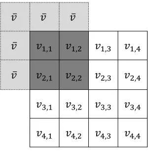
RΓ, which can be approximated as the true signalx plus i.i.d. Gaussian noise (in a sense that will be made clear in the statement of our main result, Theorem 2.2.1). Note that the sliding-windows {Λi}i∈Γ and the sliding-window denoiserηt are defined on multidimensional signals, hence we use the inverse of the vectorization operator,
V−1, to rearrange elements of vectors into arrays before applying the sliding-window denoiser
ηt. It should also be noted that the denoiser ηtmay only process part of the signal elements in Λ. For example, in the 2D case, if Λ is defined as a 3×3 window, thenηt may only process the center and the four adjacent pixel values in the window (see Figure 2.1) and ignore the four corners. To simplify notation, we will writeηt:RΛ→Rthroughout the chapter, and interpret this notation to mean that any processing of neighboring signal values is allowed, including the possibility of ignoring some of their values.
𝑖
Figure 2.1For Λ of size 3×3, the denoiserηt : RΛ → Rmay only process the pixels in gray (the center and the four adjacent pixels).
set Γ into two sets Γmid and Γedge defined as:
Γmid :={i∈Γ|Λi∩Γc=∅}, and Γedge :={i∈Γ|Λi∩Γc6=∅}. (2.8) That is, fori∈Γmid, all elements in Λiare inside Γ, whereas fori∈Γedge, some of the elements in Λi fall outside Γ.
For anyv∈RΓ, let v
Λi be a subset of the elements of v with indices in Λi. Notice that for
i∈ Γmid, all entries of vΛi are well-defined. For i∈ Γedge, vΛi has undefined entries, namely, for allj ∈Λi∩Γc,vj is not defined. We now define the value of those “missing” entries to be the average of the entries of vΛi with indices in Γ. Formally,
vj := 1
|Λi∩Γ|
X
`∈Λi∩Γ
v`, ∀j ∈Λi∩Γc. (2.9)
Notice thatvΛi for alli∈Γ are now defined by the entries in the originalv∈RΓ. To emphasize this point, which will be useful in the proof for our main result, we define a set of operators
{Ti}i∈Γ with Ti :RΛi∩Γ→RΛ defined as
Ti(vΛi∩Γ) :=vΛi, ∀i∈Γ, (2.10) wherevΛi follows our definition above for all i∈Γ. That is, Ti is identity fori∈Γmid, whereas for i ∈ Γedge, Ti extends a smaller array vΛi∩Γ to a larger one vΛi with the extended entries defined by (2.9).
ҧ
𝑣 𝑣ҧ 𝑣ҧ
ҧ
𝑣 𝑣1,1 𝑣1,2 𝑣1,3 𝑣1,4
ҧ
𝑣 𝑣2,1 𝑣2,2 𝑣2,3 𝑣2,4
𝑣3,1 𝑣3,2 𝑣3,3 𝑣3,4
𝑣4,1 𝑣4,2 𝑣4,3 𝑣4,4
Figure 2.2Illustration of the definition of “missing” entries in a sliding window inZ2. The matrix
v ∈ R4×4. The half-window size isk = 1, thus Λ = [3]×[3]. For the window Λ(1,1)centered at coordinate (1,1), the “existing” entries in the window arev1,1, v1,2, v2,1, v2,2 as shown in dark gray. Five entries, which are in light gray, are missing, hence we define their value to be the average of the existing ones, ¯v=14(v1,1+v1,2+v2,1+v2,2).
k+ 1, N −k+ 2, . . . , N} as defined in (2.8). Therefore, for alli∈Γmid, we have vΛi =Ti(vi−k, vi−k+1, . . . , vi+k) = (vi−k, vi−k+1, . . . , vi+k)∈R2k+1.
For i∈Γedge, the vectorvΛi is still length-(2k+ 1), and we set the values of the non-positive indices, i.e., 1−k,2−k, . . . ,−1,0, or indices aboveN, i.e., N+ 1, N + 2, . . . , N+k, to be the average value of the vectorvΛi with indices in Λi∩[N]. For example, leti= 3 andk= 5, then Λ3 = (−2,−1,0,1, . . . ,8). Following (2.9), define
¯
v= 1 8
8 X
j=1
vj, and set v−2 =v−1=v0 = ¯v,
hence,vΛ3 =T3(v1, . . . , v8) := (¯v,v,¯ v, v¯ 1, . . . , v8)∈R
11. An example for thep= 2 case (hence
2.2
Performance Analysis
2.2.1 Definitions and Assumptions
First we include some definitions relating to Markov random field (MRF) that will be used to state our assumptions on the unknown signal x. These definitions can be found in standard textbooks such as [46]; we include them here for convenience.
Definition 2.2.1. Let (Ω,F, P) be a probability space. A random field is a collection of random variables X = {Xi}i∈Γ defined on (Ω,F, P) having spatial dependencies, where Xi : Ω → E for some measurable state space (E,E) and Γ ⊂ Zp is a non-empty and finite subset of the infinite lattice Zp. We think of Γ as a collection of spatial locations. Denote the qth-order
neighborhood of location i∈Γ by Niq, that is, Niq ⊂Γ is a collection of location indices at a
distance less than or equal toq from ibut not including i. Formally,
Niq= n
j∈Γ\ {i} | ki−jk2 ≤q
o
.
Following these definitions, X is said to be a qth-order MRF if, for all i ∈ Γ, hence i = (i1, . . . , ip), and for all measurable subsetsB ∈ E, we have
P(Xi∈B|Xj, j∈Γ\ {i}) =P(Xi ∈B|Xj, j∈ Niq),
and for all B ∈ EΓ we have P(X ∈ B) > 0. The second positivity condition ensures that the joint distribution of a MRF is a Gibbs distribution by the Hammersley-Clifford theorem [50].
Let µ denote the distribution measure of X, namely for all B ∈ EΓ, we have P(X∈B) =
µ(B), and µΛ the distribution measure of XΛ:={Xi}i∈Λ for Λ⊂Γ. For any i∈Γ, define the seti+ Λ :={i+j|j ∈Λ}. Then the random field is said to bestationary if for alli∈Γ such thati+ Λ⊂Γ, it is true thatuΛ=ui+Λ.
Next we introduce the Dobrushin uniqueness condition, which ensures that the random field mixes sufficiently fast and leads to a unique stationary Gibbs distribution. Define the
Do-brushin interdependence matrix (Ci,j)i,j∈Γ for the distribution measure µ of the random
field X to be
Ci,j := sup
ξ,ξ0∈EΓ
ξjc=ξ0jc
kµi(·|ξ)−µi(·|ξ0)ktv. (2.11)
probability measures ρ1 and ρ2 on (E,E) is defined as
kρ1(·)−ρ2(·)ktv := max
A∈E |ρ1(A)−ρ2(A)|.
Note that if E is countable, then
kρ1(·)−ρ2(·)ktv = 1 2
X
x∈E
|ρ1(x)−ρ2(x)|. (2.12)
The measure µ is said to satisfy the Dobrushin uniqueness condition if
c:= sup i∈Γ
X
j∈Γ
Ci,j <1.
The Dobrushin contraction coefficient, c, is a quantity that estimates the magnitude of
change of the single site conditional expectations, as they appear in (2.11), when the field values at the other sites vary. Similarly, we define thetransposed Dobrushin contraction
condi-tion as
c∗:= sup j∈Γ
X
i∈Γ
Ci,j <1.
We can now state our assumptions on the signal x, the matrix A, and the noise w in the linear system (1.2), as well as the denoiser function ηt used in the algorithm (2.6) and (2.7).
Signal: Let E ⊂R be a bounded state space (countable or uncountable). Letx={xi}i∈Γ be a stationary MRF with Gibbs distribution measureµonEΓ, where Γ⊂Zpwithp= 1,2,3 is a finite and nonempty rectangular lattice. We assume thatµsatisfies the Dobrushin uniqueness condition and the transposed Dobrushin uniqueness condition as defined in 2.2.1. The class of finite state space stationary MRFs, which is widely used for image analysis [73], is one example that satisfies our assumption.
Denoisers:The denoisers ηt:RΛ→R used in (2.7) are assumed to be Lipschitz3 for each
t > 0 and are, therefore, weakly differentiable with bounded (weak) partial derivatives. We further assume that the partial derivative w.r.t. the center coordinate of Λ, which is denoted by ηt0 :RΛ→ R, is itself differentiable with bounded partial derivatives. Note that this implies
ηt0 is Lipschitz. (It is possible to weaken this condition to allow ηt0 to have a finite number of discontinuities, if needed, as in [104].)
Matrix: The entries of the matrixA are i.i.d. with distributionN(0,1/n).
3A function f :
Rm → R is Lipschitz if there exists a constant L > 0 such that for all x,y ∈ Rm,
Noise: The entries of the measurement noise vector w are i.i.d. according to some sub-Gaussian distribution pw with mean 0 and finite variance σw2. The sub-Gaussian assumption implies [17] that for all >0, there exist some constantsK, κ >0 such that
P
1
nkwk
2−σ2 w
≥
≤Ke−κn2. (2.13)
2.2.2 Main Result
As noted in Section 1.1, the behavior of the AMP algorithm is predicted by a deterministic scalar recursion referred to as state evolution, which is now formally introduced here. More specifically, the state evolution sequences {τt2}t≥0 and {σt2}t≥0 defined below in (2.14) will be used in Theorem 2.2.1 to characterize the estimation error of the estimates produced by AMP. Let the probability measureµdefine the (stationary) prior distribution for the unknown signal xin (1.2). Then by our assumption of stationarity, we havexi∼µ1 for all i∈Γ and xΛi ∼µΛ for alli∈Γmid with Γmid defined in (2.8), whereµ1andµΛdenote the one-dimensional marginal and Λ-dimensional marginal ofµ, respectively. Defineσx2 =E[x21]>0, andσ02=σx2/δ. Iteratively define{τ2
t}t≥0 and {σt2}t≥1 as follows,
τt2 =σ2w+σt2 and σt2= 1
δ|Γ|
X
i∈Γ E
h
(ηt−1(xΛi+τt−1ZΛi)−xi)2 i
, (2.14)
where ηt : RΛ → R is the sliding-window denoiser and Z= {Zi}i∈Γ has i.i.d. N(0,1) entries and is independent of x. We notice that for all i∈Γmid, x
Λi d
=x0, where x0 ={x0i}i∈Λ ∼µΛ, and [Z]Λi
d
= Z0, where Z0 ={Zi0}i∈Λ has i.i.d. N(0,1) entries. Therefore, for all i∈ Γmid, the expectations in (2.14) satisfy
E h
(ηt−1(xΛi+τt−1ZΛi)−xi)2 i
=E h
ηt−1(x0+τt−1Z0)−x0c 2i
,
where x0c is the center coordinate of x0. For i ∈ Γedge with Γedge defined in (2.8), it is not necessarily true that xΛi
d
= x0, because following the definition in (2.9) some of the entries of xΛi are defined as the average of other entries.
The explicit expression for the definition ofσ2t in (2.14) is different when considering Γ⊂Zp for different p values, because the size and the patterns of edges and corners of the set Λi for
the Λ-dimensional marginal measureµΛ instead of the joint measureµ, as demonstrated in the two examples below in (2.15) and (2.16).
Let x0c be the center coordinate of x0 and Λc the window Λ ⊂ Zp translated with center
c∈Zp. Recall that Λ is thep-dimensional cube with length (2k+ 1) in each of thepdimensions. Then we havex0 =x0Λc and when we consider shiftsx0Λc
+` for`∈ {−k,−k+ 1, . . . , k−1, k}we, analogous to the definition in (2.9), define “missing” entries to be replaced by the average of the existing entries. (Note that x0 is exactly of size Λ, thus for any` 6= 0, there will be “missing” entries.) For example, whenp= 1,
x0Λc = (x01, x02, . . . , x02k+1), while xΛc0 −2 = ( ¯x , x , x¯ 01, x02, . . . , x02k−1), where ¯x= 2k1−1P2k−1
i=1 x0i. Generalizing, we have random vector x0Λc+` of length 2k+ 1 defined as
x0Λc+`=
1 2k+1+`
P2k+1+`
i=1 x0i, . . . , 2k+1+`1
P2k+1+`
i=1 x0i, x01, x02, . . . , x02k+1+`
if` <0,
x01, x02, . . . , x02k+1 if`= 0,
x01+`, x02+`, . . . , x02k+1, 2k+11−`P2k+1
i=1+`x0i, . . . , 2k+11−`
P2k+1 i=1+`x0i
if` >0.
The same idea can be extended easily when p= 2 or p= 3.
For the case p = 1, we note that Γmid = {k+ 1, k+ 2, . . . , N −k −1} and Γedge =
{1,2, . . . , k} ∪ {N −k, N −k+ 1, . . . , N}, hence|Γmid|=N−2k and |Γedge|= 2k. Therefore, we have
σt2= (N−2k)
δN E
h
ηt−1(x0+τt−1Z0)−x0c 2i
+ 1
δN
X
`∈{−k,...,k}\{0}
E
ηt−1([x0+τt−1Z]0Λc+`)−x
0
c+` 2
, (2.15)
where{−k, . . . , k} \ {0}={−k, . . . ,−1} ∪ {1, . . . , k}. In the above the first term correspond to theN−2kmiddle indices, while the second term sums over 2k terms, which correspond to all the possible edge cases.
Therefore,
σt2= (N−2k) 2
δN2 E
h
ηt−1(x0+τt−1Z0)−x0c 2i
+ 1
δN2
X
`1,`2∈{−k,...,k}\{0}
E h
ηt−1([x0+τt−1Z0]Λc+`)−x
0
c+` 2i
+(N−2k)
δN2
X
`1∈{−k,...,k}\{0}
`2=0
E h
ηt−1([x0+τt−1Z0]Λc+`)−x
0
c+` 2i
+(N−2k)
δN2
X
`2∈{−k,...,k}\{0}
`1=0
E h
ηt−1([x0+τt−1Z0]Λc+`)−x
0
c+` 2i
, (2.16)
where we notice that there are (2k)2 terms in the second summand and 2k terms in the third and fourth summands, and that (N−N2k)2 2 +
(2k)2
N2 +
2k(N−2k) N2 +
2k(N−2k)
N2 = 1. Again, in the above
the first term sums over all the middle indices. In this case, the second term corresponds to the corner edge cases, while the third and fourth terms correspond to the edge cases in one dimension only. Note that σ2t is a function of N, but we do not explicitly represent this relationship to simplify the notation. Note also that for fixedk, the terms (2k)N22,
2k(N−2k) N2 , and
2k(N−2k)
N2 vanish
asN goes to infinity. Therefore, we have limN→∞σ2t(N) = 1δE h
(ηt−1(x0+τt−1Z0)−x0c)2 i
. Similar to [104], our performance guarantee, Theorem 2.2.1, is a concentration inequality for PL(2) loss functions at any fixed iteration t < T∗, where T∗ is the first iteration when either (σt⊥)2 or (τt⊥)2 defined in (2.37) is smaller than a predefined quantity ˆ. The precise definition of (σ⊥t )2 and (τt⊥)2 is deferred to Section 2.3.2. For now, we can understand (σt⊥)2 (respectively, (τt⊥)2) as a number that quantifies (in a probability sense) how close an estimate xt (respectively, a residual zt) is in the subspace spanned by the previous estimates {xs}s<t
(respectively, the previous residuals {zs}s<t).
Theorem 2.2.1. Under the assumptions stated in Section 2.2.1, and for fixed half window-size
k >0, then for any (order-2) pseudo-Lipschitz function φ:R2→R, ∈(0,1), and0≤t < T∗,
P 1 |Γ| X
i∈Γ
φ(xt+1i , xi)−E[φ(ηt(xΛi+τtZΛi), xi)] ≥ !
≤Kk,te−κk,tn
2
, (2.17)
where x = {xi}i∈Γ is an MRF with distribution measure µ on EΓ, Z = {Zi}i∈Γ has i.i.d.
not explicitly specified. Proof. See Section 2.3.
Remarks:
(1) The probability in (2.17) is w.r.t. the product measure on the space of the matrix A, signalx, and noise w.
(2) By choosing pseudo-Lipschitz loss function to beφ(a, b) = (a−b)2, Theorem 2.2.1 gives the following concentration result for the mean squared error of the estimates. For anyt≥0,
P
1
|Γ|kx
t+1−xk2−δσ2 t+1
≥
≤Kk,te−κk,tn
2 ,
withσ2
t+1 defined in (2.14). 2.2.3 Numerical Examples
Before moving to the proof of Theorem 2.2.1, we first demonstrate the effectiveness of the AMP algorithm with sliding-window denoisers when used to reconstruct an image x from its linear measurements acquired according to (1.2). We verify that state evolution accurately tracks the normalized estimation error of AMP, as is guaranteed by Theorem 2.2.1. We use squared error as the error metric in our examples, which corresponds to the case where the PL(2) loss functionφ
in Theorem 2.2.1 is defined asφ(a, b) := (a−b)2. We remind the reader that Theorem 2.2.1 also supports other PL(2) loss functions. Moreover, we apply AMP with sliding-window denoisers to reconstruct texture images, which are known to be well-modeled by MRFs in many cases [30, 40].
2.2.3.1 Verification of state evolution
We consider a class of stationary MRFs on Z2 whose neighborhood is defined as the eight-nearest neighbors, meaning this is a 2nd-order MRF according to the definition in Section 2.2.1. The joint distribution of such an MRF on any finite M×N rectangular lattice in Z2 has the following expression [23]:
µ(a) =P(x=a) =
QM−1 m=1
QN−1 n=1
"
am,n am,n+1
am+1,n am+1,n+1 #
QM−1 m=2
QN−1 n=2
h
am,n i
QM−1 m=2
QN−1 n=1
h
am,n am,n+1 i
QM−1 m=1
QN−1 n=2
"
am,n
Figure 2.3Numerical example. From left to right: ground-truth image generated by the MRF de-scribed in Section 2.2.3.1, image reconstructed by AMP with a separable Bayesian denoiser (computed from the incorrect assumption that the signal is generated from an i.i.d. Bernoulli distribution), and image reconstructed by AMP with a Bayesian sliding-window denoiser withk= 1, hence Λ = [3]×[3]. (Γ = [128]×[128],δ= 0.5, SNR = 17 dB.)
where we follow the notation in [23] for the generic measure "
am,n am,n+1
am+1,n am+1,n+1 #
defined as
"
am,n am,n+1
am+1,n am+1,n+1 #
:=P(xm,n =am,n, xm,n+1 =am,n+1, xm+1,n =am+1,n, xM+1,n+1=am+1,n+1),
and the conditional distribution of the element in the box given the element(s) not in the box: "
am,n am,n+1
am+1,n am+1,n+1 #
:=P(xm+1,n+1 =am+1,n+1|xm,n =am,n, xm+1,n =xm+1,n, xm,n+1=am,n+1).
The generic measure needs to satisfy some consistency conditions to ensure the Markovian prop-erty and stationarity of the MRF on a finite grid; details can be found in [23]. For convenience in simulations, we use a Π+ Binary MRF as defined in [23, Definition 7], for which the generic measure is conveniently parameterized by four parameters, namely,
[1 0 ] =p, [0 1 ] =q,
" 0 0 1 0 #
=r,
" 1 1 1 0 #
=s.
In the simulations, we set {p = 0.4, q = 0.5, r = 0.01, s = 0.4}. Using (2.11) and (2.12), it can be checked that the distribution measure of this MRF satisfies the Dobrushin uniqueness condition.
0 5 10 15 20 25 Iteration
10-4 10-2 100
MSE
state evolution k=0 state evolution k=1 empirical
Figure 2.4Numerical verification that the empirical MSE achieved by AMP with sliding-window de-noisers is tracked by state evolution. The empirical MSE is averaged over 50 realizations of the MRF (as described in Section 2.2.3.1), measurement matrix, and measurement noise. (Γ = [128]×[128],
δ= 0.5, SNR = 17 dB.)
used as an input to the estimation function in (2.7) is approximately distributed as x0+τtZ0, wherex0 ∼µΛ,Z0 has i.i.d. standard normal entries and is independent ofx0, and τt is defined in (2.14). With this property in mind, a natural choice of denoisers {ηt}t≥0 are those that cal-culate the conditional expectation of the signal given the value of the input argument, which we refer to as Bayesian sliding-window denoisers. Letv∈RΛ, for eacht≥0 we define
ηt(v) :=Ex0c
x0+τtZ0=v
, (2.18)
wherex0cdenotes the center coordinate of x0. Figure 2.4 shows that the MSE achieved by AMP with the non-separable sliding-window denoiser defined above is tracked by state evolution at every iteration.
Notice that when k= 0, the denoisers{ηt}t≥0 are separable and the empirical distribution of any realization ofxconverges to the µ1 on E⊂R. For this case, the state evolution analysis for AMP with separable denoisers (k= 0) was justified by Bayati and Montanari [7]. However, it can be seen in Figures 2.3 and 2.4 that the MSE achieved by the separable denoiser (k= 0) is significantly higher (worse) than that achieved by the non-separable denoiser (k= 1).
2.2.3.2 Texture Image Reconstruction
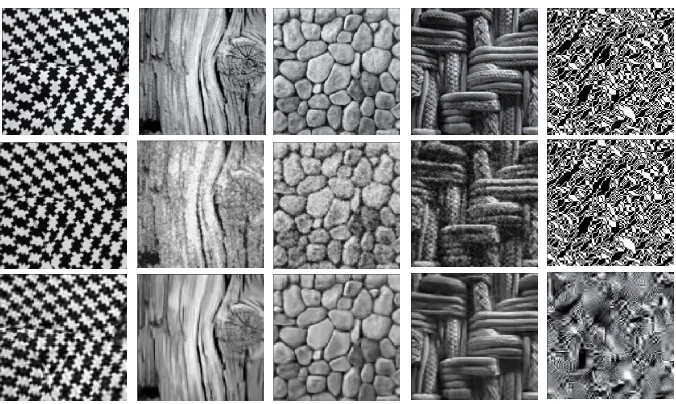
Figure 2.5Reconstruction of texture images using AMP with different denoisers. From left to right: original gray level images, binary ground-truth images, images reconstructed by AMP with a total variation denoiser [8], non-separable Bayesian sliding-window denoiser (MRF prior,k = 1), and sepa-rable Bayesian denoiser (Bernoulli prior), respectively. From top to bottom: images of cloud, leaf, and wood, respectively. (Γ = [128]×[128],δ= 0.3, SNR = 20 dB.)
model for each of these images using well-established MRF learning algorithms, we do not include this procedure in our simulations, since the study of texture image modeling is beyond the scope of this work and the reconstruction results obtained using the simple MRF defined above are sufficiently satisfactory even though the prior may be inaccurate. In Figure 2.5, we take nature images of cloud, leaf, and wood (1st column) and use thresholding to generate the binary testing images (2ndcolumn). In addition to presenting the reconstructed images obtained by AMP with the Bayesian sliding-window denoisers with k = 1 (4th column) and k= 0 (5th column), respectively, we also present those obtained by AMP with a total variation denoiser [8] as a baseline approach (3th column).
2.3
Proof of Theorem 2.2.1
2.3.1 Proof Notation
As in the work by Rush and Venkataramanan [104], as well as by Bayati and Montanari [7], the technical lemma is proved for a more general recursion, with AMP being a specific example of the general recursion. The connection between AMP and the general recursion is explained in (2.26) and (2.27).
Fix the half-window size 0 ≤ k ≤ (N −1)/2, an integer. Let {ft}t≥0 : RΛ×Λ → R and
{gt}t≥0 : R2 → R be sequences of Lipschitz functions. Specifically, the arguments of ft are two variables in RΛ, for example, for x,y ∈ RΛ, we write ft(x,y) and refer to x as the first argument offt. Given the noisewand the unknown signalx, defineR|Γ|-valued random vectors ht+1,qt+1 and
Rn-valued random vectors bt,mt, as well as RΓ-valued random fields hbt,qbt, whereht+1=V(hbt+1) andqt+1 =V(bqt+1), fort≥0 recursively as follows. Starting with initial condition bq
0∈ RΓ:
ht+1:=A∗mt−ξtqt, qt:=V(bq t), b
ht+1:=V−1(ht+1), qbti :=ft
b
htΛi,xΛi
, for all i∈Γ, bt:=Aqt−λtmt−1, mti :=gt(bti, wi), for alli∈[n],
(2.19)
with the scalarsξt, λt defined as
ξt:= 1
n
n X
i=1
gt0(bti, wi), λt:= 1
n
X
i∈Γ
ft0
b
htΛi,xΛi
, (2.20)
where the derivative of gt is w.r.t. the first argument, and the derivative of ft is w.r.t. the center coordinate of the first argument. In the context of AMP, as made explicit in (2.26), the terms bht+1 and bqt measure the error in the observation V−1(A∗zt) +xt and the estimate xt at iterationt, respectively, (the error w.r.t. the true x). The termmt measures the residual at iterationt and the termbt is the difference between the noise and residual at iteration t.
Recall that the unknown signal x is assumed to have a stationary MRF prior with distri-bution measure µon EΓ. Let 0∈RΛ be an all-zero array. Define
σ2x:=E[x21], (2.21)
σ20 := 1
δ|Γ|
X
i∈Γ
Further, for all i∈Γ let
b
qi0:=f0(0,xΛi), and q0 :=V(qb
0), (2.23)
and assume that there exist constants K, κ >0 such that
P
1
n
q0
2
−σ02
≥
≤Ke−κn2. (2.24)
Define the state evolution scalars {τt2}t≥0 and {σ2t}t≥1 for the general recursion as follows.
τt2 :=E[(gt(σtZ, W))2], σ2t := 1
δ|Γ|
X
i∈Γ
E[(ft(τt−1ZΛi,xΛi))2], (2.25)
where random variables W ∼pw and Z ∼ N(0,1) are independent, andx={Xi}i∈Γ ∼µ and Z={Zi}i∈Γ with i.i.d.N(0,1) entries are also independent. We assume that both σ20 and τ02 are strictly positive. The technical lemma will show that bht+1 can be approximated as i.i.d.
N(0, τt2) in functions of interest for the problem, namely when used as an input to pseudo-Lipschitz functions, andbtcan be approximated as i.i.d.N(0, σt2) in PL functions. Moreover, it will be shown that the probability of the deviations of the quantities n1kmtk2 and 1
nkbq
tk2 from
τt2 andσ2t, respectively, decay exponentially in n.
We note that the AMP algorithm introduced in (2.6) and (2.7) is a special case of the general recursion of (2.19) and (2.20). Indeed, define the following vectors recursively fort≥0, starting withx0 =0 and z0 =y.
b
ht+1=x−(V−1(A∗zt) +x0), bqt=xt−x,
bt=w−zt, mt=−zt. (2.26)
It can be verified that these vectors satisfy (2.19) and (2.20) using Lipschitz functions
ft(a,xΛi) =ηt−1(xΛi−a)−xi, and gt(b, wi) =b−wi, (2.27) where a ∈RΛ and b ∈ R. Using the choice of ft, gt given in (2.27) also yields the expressions for σt2, τt2 given in (2.14). In the remaining analysis, the general recursion given in (2.19) and (2.20) is used. Note that in AMP, q0 = −x and σ02 = (1/δ)σx2, hence, assumption (2.24) for AMP requires
P
1
|Γ|kxk
2−
σx2
≥δ
Under our assumptions for x as stated in Section 2.2.1, we see that (2.28) is satisfied using Lemma A.3.2 (Appendix A.3), since the function f(x) =x2 is pseudo-Lipschitz. Finally, note that if we assumeσx2 >0 andδ <∞, then the condition of strict positivity ofσ02andτ02 defined in (2.25) is satisfied.
Let [c1|c2|. . .|ck] denote a matrix with columns c1, . . . ,ck. Fort≥1, define matrices Mt:= [m0 |. . .|mt−1], Qt:= [q0|. . .|qt−1], Bt:= [b0|. . .|bt−1], Ht:= [h1|. . .|ht]. (2.29) Moreover,M0,Q0,B0,H0 are defined to be the all-zero vector.
The values mtk and qtk are projections of mt and qt onto the column space of Mt and Qt, withmt⊥:=mt−mtk,andqt⊥ :=qt−qtkbeing the projections onto the orthogonal complements of Mt and Qt. Finally, define the vectors
αt:= (αt0, . . . , αtt−1)∗, γt:= (γ0t, . . . , γtt−1)∗, (2.30) to be the coefficient vectors of the parallel projections, i.e.,
mtk := t−1 X
i=0
αtimi, qtk := t−1 X
i=0
γitqi. (2.31)
The technical lemma, Lemma 2.3.4, shows that for largen, the entries of the vectorsαt andγt
concentrate to constant values which are defined in the following section.
2.3.2 Concentrating Constants
Recall thatxis the unknown vector to be recovered andwis the measurement noise in the linear model (1.2). In this section we introduce the concentrating values for various inner products of pairs of the vectors {ht,mt,qt,bt} that are used in Lemma 2.3.4.
Let {Z˘t}t≥0 be a sequence of zero-mean jointly Gaussian R-valued random variables , and let {Zet}t≥0 be a sequence of zero-mean jointly Gaussian RΓ-valued random variables. The covariance of the two random sequences is defined recursively as follows. Forr, t≥0,i, j ∈Γ,
E[ ˘ZrZ˘t] = e
Er,t
σrσt
, E
h
[Zer]i[Zet]j i
=
˘ Er,t
τrτt, ifi=j 0, ifi6=j
where
˘
Er,t :=E h
gr(σrZ˘r, W)gt(σtZ˘t, W) i
,
e
Er,t := 1
δ|Γ|
X
i∈Γ E
h
fr(τr−1[Zer−1]Λi,xΛi)ft(τt−1[Zet−1]Λi,xΛi)
i. (2.33)
Note that both terms of the above (2.33) are scalar values and we takef0(·,xΛi) :=f0(0,xΛi), the initial condition. Moreover, Eet,t = σt2 and ˘Et,t =τt2, as can be seen by comparing (2.25) and (2.33), thus for all i∈ Γ, we have E
h [Zet]2i
i
= E[ ˘Zt2] = 1. Therefore, Zet has i.i.d. N(0,1) entries.
Next, we define matricesCet,C˘t∈Rt×tand vectorsEet,E˘t∈Rtwhose entries are{Eer,t}r,t≥0 and {E˘r,t}r,t≥0 defined in (2.33). For 0≤i, j≤t−1, define
e
Ci+1,j+1t :=Eei,j, C˘i+1,j+1t := ˘Ei,j, (2.34) and
e
Et:= (Ee0,t. . . ,Eet−1,t)∗, E˘t:= ( ˘E0,t. . . ,E˘t−1,t)∗. (2.35) Lemma 2.3.1 below shows that Cet and ˘Ct are invertible. Therefore, we can define the concen-trating values forγt and αt defined in (2.30) as
b
γt:= (Cet)−1Eet and αbt:= ( ˘Ct)−1E˘t, (2.36) as well as the values of (σ⊥t )2 and (τt⊥)2 for t >0:
(σ⊥t )2 :=σt2−(γbt)∗Eet=Eet,t−Ee∗t(Cet)−1Eet, (τt⊥)2 :=τt2−(αb
t)∗˘
Et= ˘Et,t−E˘∗t( ˘Ct)
−1E˘ t.
(2.37)
Fort= 0, we let (σ0⊥)2:=σ02 and (τ0⊥)2 :=τ02. Finally, define the concentrating values forλt+1 and ξt defined in (2.20) as
b
ξt:=E h
g0t(σtZ˘t, W) i
, bλt+1:= 1
δ|Γ|
X
i∈Γ E
h
ft0(τt[Zet]Λi,xΛi) i
. (2.38)
Lemma 2.3.1. If (σk⊥)2 and (τ⊥
Proof. The proof can be found in [104].
2.3.3 Conditional Distribution Lemma
As mentioned before, the proof of Theorem 2.2.1 relies on a technical lemma, Lemma 2.3.4, which will be stated in Section 2.3.4 and proved in Section 2.4. Lemma 2.3.4 uses the conditional distribution of the vector ht+1 given the matrices in (2.29) as well as x,w. Two forms of the conditional distribution of ht+1 will be provided in Lemmas 2.3.2 and 2.3.3, which correspond to [104, Lemma 4.3] and [104, Lemma 4.4], respectively. Lemma 2.3.3 explicitly shows that the conditional distribution of ht+1 can be represented as the sum of a standard Gaussian vector and a deviation term, where the explicit expression of the deviation term is provided in Lemma 2.3.2. Then Lemma 2.3.4 shows that the deviation term is small, meaning that its normalized Euclidean norm concentrates on zero, and also provides concentration results for various inner products involving the other terms in recursion (2.19), namely{ht+1,qt,bt,mt}.
The following notation is used. Considering two random variablesX, Y and a sigma-algebra
S, we denote the relationship thatY andXgivenS are equivalent in distribution byX|S =d Y. We represent a t×t identity matrix as It, dropping the subscript t when it is clear from the context. For a matrixAwith full column rank,PkA:=A(A∗A)−1A∗is the orthogonal projection matrix onto the column space of A, and P⊥A := I−PkA. DefineSt1,t2 to be the sigma-algebra
generated by the terms
b0, ...,bt1−1,m0, ...,mt1−1,h1, ...,ht2,q0, ...,qt2, and x,w.
Lemma 2.3.2. [104, Lemma 4.3] For the vectorht+1defined in(2.19), the following conditional distribution holds for t≥0:
h1|S1,0=d τ0Z0+ ∆1,0 and ht+1|St+1,t d =
t−1 X
r=0 b
αtrhr+1+τt⊥Zt+ ∆t+1,t, (2.39)
where Z0,Zt are R|Γ|-valued random variables with i.i.d. N(0,1) entries that are independent of the corresponding conditioning sigma algebras. The term αbti for i= 0, ..., t−1 is defined in (2.36) and the term (τt⊥)2 in (2.37). The deviation terms are
∆1,0= "
m0
√
n −τ0
!
IN −
m0
√ n P
k
q0
#
Z0+q0
q0 2
n
!−1
(b0)∗m
0
n −ξ0
q0
2
n
!
and for t >0,
∆t+1,t= t−1 X
r=0
(αtr−αbtr)hr+1+ "
mt⊥
√ n −τ
⊥
t !
IN −
mt⊥
√
n P
k
Qt+1
#
Zt
+Qt+1 Q∗
t+1Qt+1
n
−1 B∗ t+1mt⊥
n −
Q∗t+1 n
"
ξtqt− t−1 X
i=0
ξiαtiqi #!
. (2.41)
Proof. The proof can be found in [104].
Note that Lemma 2.3.2 holds only when Q∗t+1Qt+1 is invertible. The following lemma pro-vides an alternative representation of the conditional distribution ofht+1|St+1,t fort≥0, and it explicitly shows thatht+1|St+1,tis distributed as an i.i.d. Gaussian random vector withN(0, τt2) entries plus a deviation term.
Lemma 2.3.3. For t≥0, letZt∈R|Γ| be i.i.d. standard normal random vectors. Let h1pure := τ0Z0. Fort≥1, recursively define
ht+1pure= t−1 X
r=0 b
αtrhr+1pure+τt⊥Zt (2.42)
and a set of scalars{dti}0≤i≤t with d00 = 1,
dti = t−1 X
r=i
driαbtr for 0≤i≤(t−1), and dtt= 1. (2.43)
Let bht+1pure=V−1(ht+1pure)∈RΓ. Then for all t≥0 we have
(hb1pure, . . . ,hbt+1pure) d
= (τ0Ze0, . . . , τtZet), (2.44) where {Zet}t≥0 are jointly Gaussian with correlation structure defined in (2.32). Moreover,
ht+1|St+1,t =d ht+1pure+ t X
r=0
dtr∆r+1,r. (2.45)
Proof. First, we prove (2.44) by induction. For t = 1, hb1pure = τ0V−1(Z0) d
is equal in distribution to Pt−1 r=0αb
t
rτrZer+τt⊥Z, where Z ∈ RΓ is independent of Zer for all
r= 0, . . . , t−1. In what follows, we show
τ0Ze0, . . . , τt−1Zet−1, t−1 X
r=0 b
αtrτrZer+τt⊥Z !
d
= (τ0Ze0, . . . , τt−1Zet−1, τtZet).
Note that Ze0, . . . ,Zet−1,Z are all zero-mean Gaussian, and therefore so is the sum. We now study the variance and covariance ofPt−1
r=0αb t
rτrZer+τt⊥Z by demonstrating the following two results:
(1) For alli, j∈Γ,
E " t−1
X
r=0 b
αtrτr[Zer]i+τt⊥Zi
! t−1 X
r=0 b
αtrτr[Zer]j+τt⊥Zj !#
=τt2E h
[Zet]i,[Zet]j i
=
τt2 ifi=j,
0 otherwise.
(2) For 0≤s≤(t−1) and all i, j∈Γ,
E "
τs[Zes]i t−1 X
r=0 b
αtrτr[Zer]j+τt⊥Zj !#
=τsτtE h
[Zes]i,[Zet]j i = ˘
Es,t ifi=j, 0 otherwise.
First, consider (1). We note that
E " t−1
X
r=0 b
αtrτr[Zer]i+τt⊥Zi ! t−1
X
r=0 b
αtrτr[Zer]j+τt⊥Zj !#
(a) =
t−1 X
r=0 t−1 X
s=0 b
αtrαbtsτrτsE h
[Zer]i[Zes]j i
+(τt⊥)2E[ZiZj]
(b) =
Pt−1
r=0 Pt−1
s=0αb t rαb
t
sE˘r,s+ (τt⊥)2 ( c)
= τt2, ifi=j,
0, otherwise.
In the above, step (a) follows from the fact thatZis independent ofZe0, . . . ,Zet−1, step (b) from
the covariance definition (2.32) and the fact that the elements ofZare i.i.d. standard Gaussian, and step (c) from
t−1 X
r=0 t−1 X
l=0 b
αtrαbtlE˘r,l= (αb t)∗C˘t
b
Next, consider (2). We see that
E "
τs[Zes]i t−1 X
r=0 b
αrtτr[Zer]j+τt⊥Zj !#
(a) =
t−1 X
r=0 b
αtrτsτrE h
[Zes]i[Zer]j i(b)
=
Pt−1
r=0E˘s,rαb t
r, ifi=j,
0, otherwise.
In the above, step (a) follows, since Z is independent of Zes and step (b) from (2.32). Finally, notice thatPt−1
r=0E˘s,rαb t
r = [ ˘Ctαb t]
s+1= ˘Es,t, where the first equality holds, since the sum equals the inner product of the (s+ 1)th row of ˘Ct with αbt and the second equality by definition of
b
αt in (2.36).
Next, we prove (2.45), also by induction. For t= 0, by (2.39) we have ht+1|
St+1,t d
=τ0Z0+ ∆1,0
d
=h1pure+ ∆1,0. Assume that hr+1|St+1,t d
=hr+1pure+Pr
i=0dri∆i+1,i holds for r= 0, . . . , t−1 as the inductive hypothesis. Then,
ht+1|St+1,t=d t−1 X
r=0 b
αtrhr+1+τt⊥Zt+ ∆t+1,t d =
t−1 X
r=0 b
αtr hr+1pure+ r X
i=0
dri∆i+1,i !
+τt⊥Zt+ ∆t+1,t
= t−1 X
r=0 b
αtrhr+1pure+τt⊥Zt+ t−1 X r=0 r X i=0 b
αtrdri∆i+1,i+ ∆t+1,t=ht+1pure+ t X
i=0
dti∆i+1,i.
In the above, the first equality uses (2.39) and the second the inductive hypothesis. The last equality follows by noticing that Pt−1
r=0 Pr
i=0vr,i = Pt−1
i=0 Pt−1
r=ivr,i for (vi,r)0≤i,r≤t−1 and using (2.43).
2.3.4 Main Concentration Lemma
Lemma 2.3.4. We use the shorthandXn=. cto denote the concentration inequalityP(|Xn−c| ≥
)≤Kk,te−κk,tn
2
, where Kk,t, κk,t denote constants depending on the iteration index tthe fixed half-window size k, but not on n or . The following statements hold for 0 ≤ t < T∗ and
∈(0,1).
(a) For∆t+1,t defined in (2.40) and (2.41),
P
1
|Γ|k∆t+1,tk
2 ≥
![Figure 2.5 Reconstruction of texture images using AMP with different denoisers. From left to right:original gray level images, binary ground-truth images, images reconstructed by AMP with a totalvariation denoiser [8], non-separable Bayesian sliding-window](https://thumb-us.123doks.com/thumbv2/123dok_us/1711471.1217570/28.612.139.475.102.306/reconstruction-dierent-denoisers-reconstructed-totalvariation-denoiser-separable-bayesian.webp)