RECENT ADVANCES IN SPARSE DIRECT SOLVERS
Emmanuel Agullo1, Patrick R. Amestoy2, Alfredo Buttari3, Abdou Guermouche4,
Guillaume Joslin5, Jean-Yves L’Excellent6, Xiaoye S. Li7, Artem Napov8, François-Henry Rouet7, Mohamed Sid-Lakhdar6, Shen Wang9, Clément Weisbecker2, and Ichitaro Yamazaki10 1INRIA/LaBRI, Bordeaux, France.
2
Université de Toulouse, INPT(ENSEEIHT)-IRIT, Toulouse, France.
3CNRS-IRIT, Toulouse, France. 4
Université Bordeaux 1/LaBRI, Bordeaux, France.
5CERFACS, Toulouse, France. 6
INRIA-LIP, ENS Lyon, Lyon, France.
7
Lawrence Berkeley National Laboratory, Berkeley, CA, USA.
8Université Libre de Bruxelles, Bruxelles, Belgium. 9
Center for Computational and Applied Mathematics, Purdue University, West Lafayette, IN, USA.
10University of Tennessee, Knoxville, TN, USA.
ABSTRACT
Direct methods for the solution of sparse systems of linear equations of the formA x=bare used in a wide range of numerical simulation applications. Such methods are based on the decomposition of the matrix into a product of triangular factors (e.g.,A=L U), followed by triangular solves. They are known for their numerical accuracy and robustness but are also characterized by a high memory consumption and a large amount of computations. Here we survey some research directions that are being investigated by the sparse direct solver community to alleviate these issues: memory-aware scheduling techniques, low-rank approximations, and distributed/shared memoryhybrid programming.
INTRODUCTION
Context and objectives
Large sparse linear systems appear in numerous scientific applications. For example, the structural analysis of nuclear plants after the Fukushima events (March 2011) requires to solve large linear systems with typically tens or hundreds of millions of unknowns arising from numerical simulation at very large scale (an entire plant structure), and in very high resolution. Direct methods for the solution of sparse linear systems are known for their numerical robustness but usually have large computational requirements (as opposed to iterative methods). In particular, their large memory footprint often prevents their use, and achieving large scale parallelism (thousands of cores or more) is often difficult. Here we survey some recent techniques that aim at improving the scalability of direct methods. In the first section, we describe amemory-aware schedul-ing strategy that aims at improvschedul-ing the memory scalability of a variant of sparse Gaussian elimination called themultifrontal method. In the second section, we introduce different low-rank approximationtechniques that aim at decreasing the space and time complexity of direct solvers by detectingdata sparsityand intro-ducing controlled approximations. Finally, in the last section, we show how to combinedistributed-memory
andshared-memory parallelismin order to exploit recent architectures.
Background
more detail. We are to compute a factorization of a given matrixA,A=L U if the matrix is unsymmetric, orA=L D LT if the matrix is symmetric. Without loss of generality, in the rest of the paper we will assume thatAis non-reducible. For a matrixAwith an unsymmetric pattern (nonzero structure), we assume that the factorization takes place using the structure ofA+AT, where the summation is structural. The fundamental structure on which we will rely in the following is called the elimination tree. A few equivalent definitions are possible (we recommend the survey by Liu (1990)); we use the following:
Definition 1 Assume A = L U where A is a sparse, structurally symmetric, N ×N matrix. Then, the elimination tree ofAis a tree ofN nodes, with thei-th node corresponding to thei-th column ofLand with the parent relations defined by:
parent(j) =min{i:i > j andℓij ̸= 0}, forj= 1, . . . , N−1
In practice, nodes areamalgamated: nodes that represent columns and rows of the factors with similar structures are grouped together in a single node (often referred to as asupernode). The elimination tree is a workflow and dataflow graph for many direct methods. At this point, two main variants of sparse direct methods can be distinguished. In themultifrontal method (Duff & Reid (1983)), each node in the elimination tree is associated with a square dense matrix (referred to as afrontal matrixorfront) with the following2×2block structure: [
F11 F12
F21 F22 ]
We refer to the variables associated withF11andF22as thefully-summedandnon fully-summedvariables,
respectively. Factoring the matrix using the multifrontal method consists in a bottom-up traversal of the tree, following a topological order (a node is processed before its parent). Processing a node consists in:
• forming (orassembling) the frontal matrix by summing the rows and columns ofAcorresponding to the variables in the(1,1)block with temporary data that has been produced by the child nodes; • eliminating the pivots in the(1,1)blockF11: this is done through a partial factorization of the frontal
matrix which produces the corresponding rows and columns of the factors stored inF11,F21andF12.
At this step, the so-called Schur complement orcontribution blockis computed asF22←F22−F21·
F11−1·F12and stored in a temporary memory; it will be used to form the front associated with the parent
node. Therefore, when a node is activated, it “consumes” the contribution blocks of its children. In the multifrontal method, theactive memory(at a given step in the factorization) consists of the front being processed and a set of contribution blocks that are temporarily stored and will be consumed at a later step.
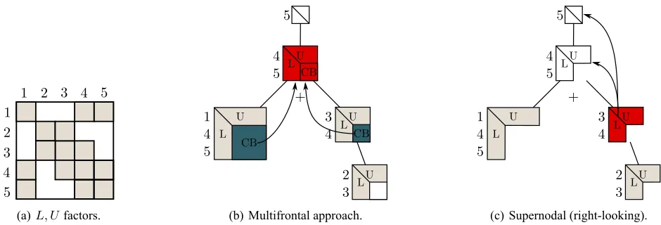
Supernodal methodscan also rely on the elimination tree, however a node in the tree is not associ-ated with a dense matrix but simply with some columns and rows of the factors. There is no contribution block. Instead, the updates corresponding to a node are done by communicating pieces of factors to some of its ancestors or from some of its descendants (right-looking orleft-lookingapproach, respectively). The multifrontal method usually exhibits good flop rates as it mainly consists of large BLAS 3 operations (for computing contribution blocks), and it has a simple communication pattern (from children nodes to their parent), but the abovementioned active memory can be quite large. Supernodal methods do not have this extra memory usage but they have more complicated communication patterns. We illustrate the difference between these two classes of methods in Figure 1.
1 2 3 4 5 1
2 3 4 5
(a)L, Ufactors.
5
5 4
1 4 5
3 4
2 3 +
CB
CB CB
L L
L L
U U
U
U
(b) Multifrontal approach.
5
5 4
1 4 5
3 4
2 3 +
L L
L L
U U
U
U
(c) Supernodal (right-looking).
Figure 1: (a) Structure of theL, Ufactors of a5×5matrix; shaded elements are nonzeros. (b) Multifrontal approach: when a node is activated (in red), it consumes the contribution blocks of its children from the stack memory. (c) Supernodal (right-looking approach): once some rows (columns) ofL(U) are computed (in red), they are sent to the ancestors that need them. Gray nodes are processed before the red node.
Many software packages implement parallel sparse direct methods. We report on experiments with two widely-used solvers: the multifrontal code MUMPS (MUltifrontal Massively Parallel Solver, (Amestoy et al. (2001)) and the supernodal code SuperLU_DIST (Li & Demmel (2003)).
MEMORY-AWARE MAPPING AND SCHEDULING TECHNIQUES
In this section we focus on the multifrontal method, although similar ideas could be applied to other variants. In the multifrontal method, the active memory (mentioned in the previous section) can be quite large and is often difficult to control in a parallel environment. We are interested in maximizing the memory efficiency emax(p) = p·SSseqmax where Sseq is the peak of active memory for a sequential execution, and
Smaxis the maximum peak of active memory for an execution onpprocessors. emax(p)should be close to
1, which means that the peak of a given processor should be close to Sseq
p . Smaxdepends on the
node-to-process mapping followed during the factorization. Commonly-used mappings often rely on theproportional mapping; in this strategy, the processors assigned to a node of the elimination tree are distributed to its children proportionally to their weights (operation count or sequential peak of memory). For example, the tree shown in Figure 2(a) is mapped on 64 processors. Its child node “a” is mapped on 70+50+5070 ·64 = 26 processors. The three subtrees rooted at a, b, and c, are mapped on different processors and are processed in parallel. In this example, the maximum peak of active memory isat least 7026GB (which is reached in the ideal case where the efficiency in the subtree rooted at a is 1), which yieldsemax ≤ 6480·70
26
= 0.40, which is
far from 1.
We proposed amemory-awaremapping technique that aims at enforcing a user-given memory con-straintM0which is the maximum allowed peak of active memory of a processor. The basic idea is to follow
a proportional mapping and to reject the steps that lead to violate the memory constraint. Take Figure 2(a) and assumeM0 = 1.6GB. As explained above, the memory peak for the subtree rooted at a is at least7026GB,
which is greater thanM0. Our memory-aware strategy is illustrated in Figure 2(b): instead of mapping the
whole set of siblings using proportional mapping, we detect groups of siblings (here{a}and{b, c}) that can be mapped using proportional mapping without violatingM0. We enforce scheduling constraints that
force these groups to start one after another (here the subtrees rooted at nodes b and c cannot start before the subtree rooted at a is completed). Here the efficiency becomes at least Sseq
p·M0 = 80
70 GB 50 GB 50 GB 80 GB
r
a b c
19 64
26 19
(a) Proportional mapping.
70 GB 50 GB 50 GB 80 GB
r
a b c
32 64
64 32
(b) Memory-aware mapping.
Figure 2: Mapping strategies. Sequential peaks of active memory are in black. The number of processors associated with each subtree is in red. In (b), the arrow is a scheduling constraint.
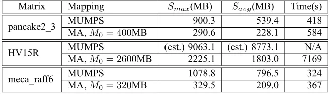
In Table 1, we provide results for 3 benchmark matrices. pancake2_3 is from a 3D problem in electromagnetism, HV15R is from computational fluid dynamics, and meca_raff6 is a thermo-mechanical coupling problem for EDF nuclear power plants. We compare the default scheduling strategy in MUMPS with our memory-aware scheduling. The results show that the active memory can be significantly reduced, at the price of a moderate increase in run time. The missing data for HV15R means that the factorization with the default scheduling ran out of memory (we show an estimated memory consumption).
Table 1: Comparison of the default strategy in MUMPS and the memory-aware algorithm.
Matrix Mapping Smax(MB) Savg(MB) Time(s)
pancake2_3 MUMPS 900.3 539.4 418
MA,M0= 400MB 290.6 228.1 584
HV15R MUMPS (est.) 9063.1 (est.) 8773.1 N/A
MA,M0= 2600MB 2225.1 1803.0 7169
meca_raff6 MUMPS 1078.8 796.5 324
MA,M0= 320MB 329.5 209.0 367
We refer the reader to (Rouet (2012)) for a more detailed description and more results.
LOW-RANK APPROXIMATIONS
Matrices coming from elliptic Partial Differential Equations (PDEs) have been shown to have a low-rank property: well defined off-diagonal blocks of their Schur complements can be approximated by low-rank products. Given a suitable ordering of the matrix, such approximations can be computed using truncated SVD or rank-revealing QR factorizations, given a low-rank truncation parameterε. The resulting representation offers a substantial reduction of the memory requirements and many of the basic dense algebra operations can be performed with less operations. Even whenεis set to maintain full accuracy (e.g.,ε = 10−14for double-precision arithmetic) dramatic savings can be obtained both in memory consumption and in complexity of a sparse factorization; alternatively, with bigger threshold values, approximated factorizations can be computed for example to precondition iterative solvers at a cost which is only a fraction of the cost of a standard, full-rank factorization. Here we present two low-rank representations that can be embedded within sparse direct solvers: Block Low-Ranktechniques andHierarchically Semi-Separablerepresentations.
Block Low-Rank techniques
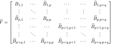
defined by conveniently clustering the associated unknowns. A BLR representation of a frontF is shown in equation from Figure 3(a) where we assume thatpsubblocks have been defined over the fully-summed variables part of F, and q subblocks over the non fully-summed variables part. Subblocks Bei,j of size
mi,j×ni,j and numerical rankki,j(ε)are approximated by a low-rank productUi,jVi,jT at accuracyε. Note
that diagonal subblocksBi,iare never approximated because they are assumed to be full-rank.
e F=
B1,1 · · · Be1,p · · · · · · Be1,p+q ..
. . .. ... ... ... ... e
Bp,1 · · · Bp,p · · · · · · Bep,p+q ..
. · · · · · · Bep+1,p+1 · · · Bep+1,p+q ..
. . .. ... ... . .. ... e
Bp+q,1 · · · Bep+q,p Bep+q,p+1 · · · Bep+q,p+q
(a) BLR matrix definition. (b) Structure of a BLR matrix. The
lighter a block is, the smaller is its rank.
Figure 3: BLR matrix definition and structure example.
In order to achieve a satisfactory reduction in both complexity and memory footprint, subblocks have to be chosen to be as low-rank as possible (e.g., with exponentially decaying singular values) which can be achieved by clustering the unknowns in such a way that anadmissibility condition (see Bebendorf (2008)) is satisfied. This condition states that a subblockBei,j, interconnecting variables ofiwith variables
ofj, will have a low rank if variables ofiand variables ofjarefar awayin the domain, intuitively, because the associated variables are likely to have a weak interaction. In practice, the fully-summed variables of each front are grouped by partitioning (with a tool such as METIS) the related adjacency graph whereas the non fully-summed variables are grouped using a partitioning induced by those of the fully-summed variables of ancestor nodes (see Amestoy et al. (2012)). Although compression rates may not be as good as those achieved with hierarchical formats such as those described in the next section1, BLR offers a good flexibility thanks to its simple, flat structure. In a parallel environment, this allows for an easier distribution and handling of the frontal matrices. Also, numerical pivoting can be more easily done within a BLR matrix without perturbing much the structure. Lastly, converting a matrix from the standard representation to BLR andvice versa, is much cheaper with respect to the case of hierarchical matrices. This allows to switch back and forth from one format to the other whenever needed at a reasonable cost; this is, for example, done to simplify the assembly operations that are extremely complicated to perform in any low-rank format. All these points make BLR easy to adapt to any multifrontal solver without a complete rethinking of the code.
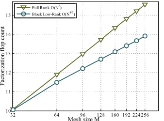
As shown in Figure 4, the O(N2) complexity of a standard, full rank solution of a 3D problem
(ofN unknowns) from an 11-point stencil is reduced toO(N4/3)when using the BLR format. In Table 2, we report results on two matrices from real-life application: Geoazur128 is a 3D seismic wave propagation study and TH_RAFF7 is a 3D thermal test-case in structural engineering for EDF nuclear power plants. The results show that the number of operations and the memory peak can be substantially reduced.
Detailed information about these techniques can be found in Amestoy et al. (2012).
Hierarchically Semi-Separable matrices
Hierarchically semi-separable (HSS) matrices (Vandebril et al. (2005)) are another type of low-rank representation that can be embedded within a sparse solver. The resulting HSS-sparse factorization can be used as a direct solver or preconditioner depending on the application’s accuracy requirement and the char-acteristics of the PDEs. If the randomized sampling compression technique is employed in compression, we
1
32 64 96 128 160 192 224256 10 11 12 13 14 15
Mesh size M
Factorization f
lop count
Full Ra nk O(N2)
Block Low-Rank O(N4/3)
Figure 4: Operation count of the BLR multifrontal factorization of a matrix coming from the Laplacian operator discretized with a 3D 11-point sten-cil, revealing a O(N4/3) complexity forε= 10−14.
Geoazur128 TH_RAFF7
ε %LU %peak %flop CSR %LU %peak %flop CSR
1×10⁻² 43.2 16.2 29.8 7.34×10⁻¹ 13.0 15.0 00.8 9.39×10⁻²
1×10⁻⁴ 50.6 17.1 31.4 4.68×10⁻³ 18.6 15.6 01.9 1.46×10⁻²
1×10⁻⁶ 64.7 30.2 45.2 7.91×10⁻⁵ 25.2 16.2 04.1 1.35×10⁻⁴
1×10⁻⁸ 78.0 46.5 62.5 3.97×10⁻⁷ 31.6 17.0 07.2 9.91×10⁻⁷
1×10⁻¹⁰ 89.1 63.9 80.4 2.07×10⁻⁹ 37.5 18.0 10.7 7.30×10⁻⁹
1×10⁻¹² 96.1 79.4 93.7 1.69×10⁻¹¹ 43.9 20.4 15.1 6.34×10⁻¹¹
1×10⁻¹⁴ 99.1 90.7 99.9 1.86×10⁻¹² 50.2 25.5 20.1 7.08×10⁻¹³
Table 2: Compression rates obtained with various values ofε. %LU is the percent of regular multifrontal (full-rank, “FR”) stor-age needed to store the BLR factors. %peak is the percent of FR maximum active memory needed to perform the BLR factoriza-tion. %flop is the percent of FR number of operations needed to perform the BLR factorization.
can show that for the 3D model problems, the HSS-sparse factorization costsO(N)flops for discretized ma-trices from certain PDEs andO(N4/3)for broader classes of PDEs (including non-selfadjoint and indefinite discretized PDEs; cf., Xia (2012)). This complexity is much lower than theO(N2)cost of the traditional, exact sparse factorization method.
Informally, the HSS representation partitions the off-diagonal blocks of a dense matrix in a hierar-chical fashion; these off-diagonal blocks are approximated by compact forms, such as truncated SVD. A key property of HSS is that the orthogonal bases are desired to benestedfollowing the hierarchical partitioning. This leads to asymptotically fast construction and factorization algorithms. Figure 5 illustrates a block8×8 HSS representation ofA, for which the hierarchical structure and the generatorsUi, Vi, Ri, andBiare
suc-cinctly depicted by the HSS tree on the right side. As a special example, its leading block4×4part looks like the following, wheret7 is the index set associated with node 7 of the HSS tree:
A|t7×t7≈
(
D1 U1B1V2H
U2B2V1H D2
) (
U1R1
U2R2
) B3
( WH
4 V4H W5HV5H
) (
U4R4
U5R5
) B6
(
W1HV1H W2HV2H) (
D4 U4B4V5H
U5B5V4H D5
) D1 D2 D4 D5 D8 D9 D11 D12 U3B3V6H 7 B14
H
U6B6V3H
B
U7 U3R3 U6R6
=
(a)8×8HSS matrix.
.. 15. 7 . 3 . 1 . 2 . 6 . 4 . 5 . 14 . 10 . 8 . 9 . 13 . 11 . 12
(b)8×8HSS tree.
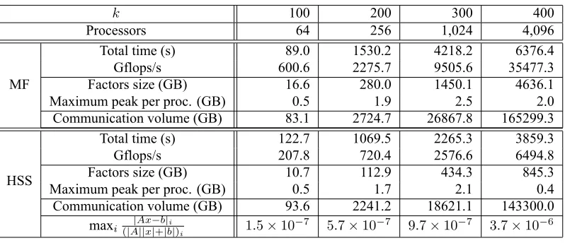
approximation algorithms to the dense submatrices in the sparse multifrontal and supernodal factorization algorithms. We report on some results using a multifrontal code specialized in the solution of the discretized Helmholtz equation on regular grids; matrices are complex, unsymmetric, highly-indefinite, and in single-precision arithmetic. We compare runs with the same code in a classical multifrontal mode, and in the HSS-sparse mode (the tolerance isε= 10−4). We solve for one right-hand side and apply iterative refinement in the solution. Using HSS techniques speeds up the solution process, and gains increase with the size of the problem, which is expected since, for this kind of equations, the complexity isO(N4/3)instead ofO(N2)for a full-rank approach. However the flop rates are smaller which is due to the fact that HSS kernels operate on small blocks, while regular kernels only perform large BLAS3 operations. The size of factors is significantly reduced but the gains on the maximum peak of memory are not as large because this particular code does not apply HSS techniques on contribution blocks (this is work in progress). The communication volume is also reduced when HSS kernels are used. Finally, using iterative refinement, the HSS-enabled code is almost as stable as the pure multifrontal code (the scaled residual is close to machine precision).
Table 3: Solution of the discretized Helmholtz equation on ak×k×kgrid.
k 100 200 300 400
Processors 64 256 1,024 4,096
MF
Total time (s) 89.0 1530.2 4218.2 6376.4 Gflops/s 600.6 2275.7 9505.6 35477.3 Factors size (GB) 16.6 280.0 1450.1 4636.1 Maximum peak per proc. (GB) 0.5 1.9 2.5 2.0 Communication volume (GB) 83.1 2724.7 26867.8 165299.3
HSS
Total time (s) 122.7 1069.5 2265.3 3859.3 Gflops/s 207.8 720.4 2576.6 6494.8 Factors size (GB) 10.7 112.9 434.3 845.3 Maximum peak per proc. (GB) 0.5 1.7 2.1 0.4 Communication volume (GB) 93.6 2241.2 18621.1 143300.0
maxi(|A|Ax||x−|+b||bi|)
i 1.5×10
−7 5.7×10⁻⁷ 9.7×10⁻⁷ 3.7×10⁻⁶
INTRODUCING SHARED-MEMORY PARALLELISM IN DISTRIBUTED-MEMORY SOLVERS
Recent architectures often consist of increasingly complex shared-memory nodes. Using distributed-memory programming(task parallelism, e.g., with MPI) within such nodes is not the best way to exploit them since they tend to have smaller and smaller amounts of per-core memory and non-uniform memory accesses (NUMA). It is thus necessary to combine distributed-memory programming for inter-node computations withshared-memory programming(thread parallelism, e.g., with OpenMP) for intra-nodes computations. Here we describe recent work carried out in MUMPS and SuperLU_DIST on this topic.
Improvement of shared-memory parallelism in distributed-memory multifrontal methods
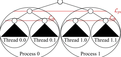
In order to exploit shared-memory parallelism at the thread level, the simplest approach consists in making many cores collaborate on the same node of the elimination tree, using multithreaded BLAS and OpenMP directives to parallelize the work outside the BLAS calls (fork-join model). This approach is gen-erally efficient, especially on large 3D problems. In order to go further, it is interesting to also exploit tree parallelism in shared-memory environments. In distributed-memory parallelism, a commonly-used tech-nique consists in defining a separating layer in the treeLps such that both tree and node parallelism are
en-vironments with the A L0 algorithm (L’Excellent and Sid-Lakhdar (2012)), that computes a layerLthsuch
that only node parallelism is applied aboveLthbut tree parallelism is now applied below it (see Figure 6).
...
.
Lps
.
Process 0
.
Process 1
.
Lth .
Lth
.
Thread 0.0
.
Thread 0.1 .
Thread 1.0 .
Thread 1.1
Figure 6: LayersLpsandLthto exploit tree parallelism in distributed and shared memory environments.
In multi-core environments, NUMA (Non-Uniform Memory Access) architectures allow for a hi-erarchical organization of memory banks. On such architectures, it is critical for performance to take into account memory affinity and memory allocation policies. By default, thelocalallocpolicy, which con-sists in mapping the memory pages on the local memory of the processor that first touches them, is applied. However, several other policies exist. Among them, theinterleavepolicy consists in allocating the mem-ory pages on all memmem-ory banks in a round-robin fashion, such that the allocated memmem-ory is spread over all the physical memory. Applying thelocalallocpolicy on data structures belowLth, in order to achieve a
better data locality and cache exploitation, and theinterleavepolicy on the ones used aboveLth, in order
to improve the bandwidth, has a dramatic effect on performance, as summarized in Table 4 when only 1 MPI process is used. This table also shows that the use of OpenMP directives to parallelize the work outside BLAS calls provides some gains, compared to the sole use of multithreaded BLAS.
On matrices such as Serena (Table 4), the sole effect of the A L0 algorithm is not so large (1081.42 seconds down to 893.64 seconds). However, the effect of memory interleaving withoutLthis even smaller
(1081.42 seconds down to 1006.66 seconds). The combined use of A L0 and memory interleaving brings a huge gain: 1081.42 seconds down to 530.63 seconds (increasing the speed-up from 7.3 to 14.7 on 24 cores). Hence, on large matrices, the main benefit of A L0 is to make the interleaving become very efficient by applying it only aboveLth. This also shows that, in the implementation, it is critical to separate the work
arrays for local threads belowLthand for the more global approach in the upper part of the tree, allowing the
application of different memory policies below and aboveLth(localallocandinterleave, respectively).
Table 4: Factorization times in seconds and effects of theinterleavememory allocation policy with node parallelism and with A L0 on an AMD 24 cores (Istanbul) system using MUMPS with a single MPI process.
Node parallelism only
Threaded ThreadedBLAS A L0 Serial BLAS +OpenMP algorithm Matrix reference Interleaving Interleaving Interleaving
off on off on off on AUDI 1535.8 269.8 260.8 231.8 225.5 158.0 110.0
conv3D64 3001.4 518.5 563.1 497.5 496.9 439.0 303.6
Serena 7845.4 1147.6 1058.0 1081.4 1006.7 893.7 530.6
These results show important aspects that should be considered inside a shared-memory node. Tun-ing the specific shared-memory factorization kernels inside each computTun-ing node is another aspect that should be considered to further improve performance. Optimizing the number of threads inside each MPI process can also have a significant impact on performance.
Multithreaded Schur-complement update in SuperLU_DIST
The distributed-memory sparse direct solver SuperLU_DIST (Li & Demmel, 2003) was initially designed to use only MPI to exploit task parallelism. In SuperLU_DIST, the computational cost of numerical factorization is typically dominated by the trailing submatrix update, where each process updates several independent blocks of the trailing submatrix at each step. Recently, we incorporated light-weight OpenMP threads in each MPI process to update disjoint sets of the independent blocks in parallel. There are several options as to how to assign the independent blocks to the threads. We use a combination of 1D/2D assignment of blocks to threads. When the number of columns of the trailing submatrix is greater than the number of threads, a process can assign its local supernodal columns to the threads in a 1D block fashion; i.e., thet-th thread updates(t−1)·h-th to(t·h−1)-th columns, whereh = nc
nt, nt is the number of threads, and
ncis the number supernodal columns assigned to this process (see Figure 7(a)). Since these columns are
contiguous in memory, each thread can access the columns with a relatively small stride. However, with this layout, the number of usable threads is constrained by the number of columns. Therefore, when the number of columns is smaller than the number of threads, we divide the columns row-wise as well, then assign the blocks to threads in a 2D cyclic fashion; namely the(i, j)-th block is assigned to(br·tc+bc)-th thread,
where the threads are organized into atr×tcgrid (i.e.,nt =tr·tc),br =mod(i, tr), andbc=mod(j, tc)
(see Figure 7(b)). Since the blocks assigned to a thread are not contiguous in memory, accessing these blocks incurs some overhead. The advantage is that it offers more parallelism than the 1D layout.
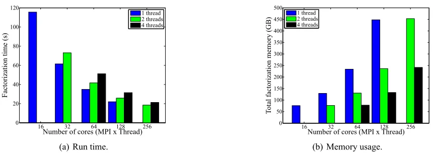
This hybrid programming paradigm obtained significant reduction in memory usage while achieving the same level of parallel efficiency as the pure MPI paradigm. As a result, in comparison to the pure MPI paradigm which failed due to the per-core memory constraint, this hybrid paradigm could use more cores on each node and reduce the factorization time on the same number of nodes.
0 0 0
0 0 0
0 0 0
1 1 1
1 1 1
1
1 1
2 2 2
2 2 2 2 2
2 2 2
3 3 3
3 3 3 3
3 3 3
1 1 1
1 1 1
1 1 1
0 0 0
0 0 0
0 0 0
2 2 2
2 2 2
2 2 2
3 3 3
3 3 3
3 3 3
(a) 1D block column layout.
0 0 0
0 0 0
0 0 0
1 1 1
1 1 1
1
1 1
2 2 2
2 2 2 2 2
2 2 2
3 3 3
3 3 3 3
3 3 3
1 1 1
1 1 1
1 1 1
0 0 0
0 0 0
0 0 0
2 2 2
2 2 2
2 2 2
3 3 3
3 3 3
3 3 3
(b) 2D cyclic layout.
Figure 7: Mapping of threads to supernodal blocks. The light-blue blocks represents the non-empty blocks in the current panel. Four MPI processes are assigned to blocks in a2×2grid, where the numbers inside the blocks indicate the process ID. Each MPI process generates four threads; the blue, green, red and yellow blocks are assigned to the first, second, third and fourth thread of process1, respectively.
be seen in the following MPI/thread configurations:32×1,32×2and32×4.
More detailed algorithm description and performance analysis appeared in Yamazaki & Li (2012).
16 32 64 128 256
0 20 40 60 80 100 120
Factorization t
ime (s)
1 thread 2 threads 4 threads
Number of cores (MPI x Thread)
(a) Run time.
16 32 64 128 256
0 50 100 150 200 250 300 350 400 450 500
Number of cores (MPI x Thread)
Total fa
ctorization memory
(GB
) 1 thread2 threads 4 threads
(b) Memory usage.
Figure 8: Time and memory using 16 nodes with various combinations of MPI tasks and OpenMP threads. REFERENCES
Amestoy, P. R., Duff, I. S., Koster, J. and L’Excellent, J.-Y. (2001). “A Fully Asynchronous Multifrontal Solver Using Distributed Dynamic Scheduling”,SIAM Journal on Matrix Analysis and Applications, 23(1), 15–41.
Amestoy, P. R., Ashcraft, C., Boiteau, O., Buttari, A., L’Excellent, J.-Y. and Weisbecker, C. (2012). “Im-proving Multifrontal Methods by Means of Block Low-Rank Representations”, Tech. Rep. RT/APO/-12/6, INRIA/RR-8199, Institut National Polytechnique de Toulouse, Toulouse, France. Submitted for publication in SIAM Journal on Scientific Computing.
Bebendorf, M. (2008). “Hierarchical Matrices: A Means to Efficiently Solve Elliptic Boundary Value Prob-lems (Lecture Notes in Computational Science and Engineering)”, Springer.
Chandrasekaran, S., Gu, M. and Pals, T. (2006). “A Fast ULV Decomposition Solver for Hierarchically Semiseparable Representations”,SIAM Journal on Matrix Analysis and Applications, 28(3), 603–622. Duff, I. S. and Reid, J. K. (1983). “The Multifrontal Solution of Indefinite Sparse Symmetric Linear
Sys-tems”,ACM Transactions on Mathematical Software, 9, 302–325.
L’Excellent, J.-Y. and Sid-Lakhdar, M. W. (2013) “Introduction of Shared-Memory Parallelism in a Distributed-Memory Multifrontal Solver”, Tech. Rep. INRIA/RR-8227. Submitted for publication. Li, X. S. and Demmel, J. W. (2003). “SuperLU_DIST: a Scalable Distributed-Memory Sparse Direct Solver
for Unsymmetric Linear Systems”,ACM TOMS, 29(2), 110–140.
Liu, J. W. H. (1990). “The Role of Elimination Trees in Sparse Factorization, SIAM Journal on Matrix Analysis and Applications, 11, 134–172
Rouet, F.-H. (2012). “Memory and Performance Issues in Parallel Multifrontal Factorizations and Triangular Solutions with Sparse Right-Hand Sides”, PhD thesis, INP Toulouse, France.
Vandebril, R., and Van Barel, M., and Golub, G. and Mastronardi, N. (2005). “A Bibliography on Semi-Separable Matrices”,Calcolo, 42, 249–270.
Wang, S., and Li, X. S., and Rouet, F.-H., and Xia, J, and V. de Hoop, M. (2013). “A Parallel Fast Geometric Multifrontal Solver Using Hierarchically Semiseparable Structure”. Submitted to TOMS.
Xia, J. (2012). “Efficient Structured Multifrontal Factorization for General Large Sparse Matrices”. SIAM Journal on Scientific Computing, revised.