SEISMIC SSI ANALYSIS OF US EPR
TMNUCLEAR ISLAND
USING DIRECT METHOD
Tobias Richter1, Calvin Wong2, and Brian Loseke3
1
Engineer, AREVA Inc., Santa Clara, CA, U.S.A. 2
Advisory Engineer, (retired) AREVA Inc., Santa Clara, CA, U.S.A. 3
Engineering Manager, AREVA Inc., Charlotte, NC, U.S.A.
ABSTRACT
The AREVA US EPR™ is a pressurized water reactor that is currently under licensing review by the US NRC. The US EPR™ Nuclear Island (NI) is founded on a common basemat supporting the Reactor Building (RB), Reactor Containment Building (RCB), Fuel Building (FB), and Safeguard Buildings (SB) 1 through 4. The Nuclear Auxiliary Building (NAB), on a separate foundation, is in close proximity to the NI as well. Detailed finite element (FE) models are developed for each of the individual buildings to support static analysis and design. For SSI analysis the afore-mentioned building models are combined into one large soil-structure interaction (SSI) model. More than 45,000 interaction nodes are defined to represent the embedded NI structures in the SASSI model so that it achieves a sufficiently high seismic wave passing frequency. High performance computing (HPC) software and data centers are used to process the complex SSI FE models for seismic analysis.
The purpose of this paper is to present the results of seismic SSI analysis of the US EPR™ NI. The analysis is performed using three modeling techniques: Subtraction Method (SM), Modified Subtraction Method (MSM), and Direct Method (DM). The results of the detailed FE model are shown in terms of transfer functions (TF), in-structure response spectra (ISRS), and total foundation seismic demand. The Direct Method results are compared against those of the Subtraction and Modified Subtraction Methods.
INTRODUCTION
As a result of review of recent applications for new reactors for Design Certification (DC) and site-specific Combined License (COL), the US NRC has identified a number of technical issues related to seismic analysis and structural design. These issues have led to issuance of more Requests for Additional Information (RAIs) for applicants. One such issue has been the use of the SASSI Subtraction Method to analyze seismic SSI response of nuclear power plants. Based on recent analyses performed for certain US Department of Energy (DOE) facilities [1], it has been found that the application of the SM to embedded structures with certain basement configurations may result in erroneous and un-conservative SSI responses as compared to using the more reliable DM in SASSI [2].
The purpose of this paper is to present the results of seismic SSI analysis of the US EPR™ NI performed using SM, MSM, and DM, with each method utilizing High Performance Computing (HPC) capabilities. The SASSI module ANALYS was modified for this work to significantly increase
ANALYTICAL METHODOLOGY
Soil-structure interaction analyses were performed using an advanced version of the SASSI code. SASSI [2] uses the finite element and complex frequency response method to calculate dynamic SSI responses of structures supported in horizontally layered soils system over uniform half-space. The primary soil material nonlinearity is the strain-compatible soil shear modulus and damping ratios.
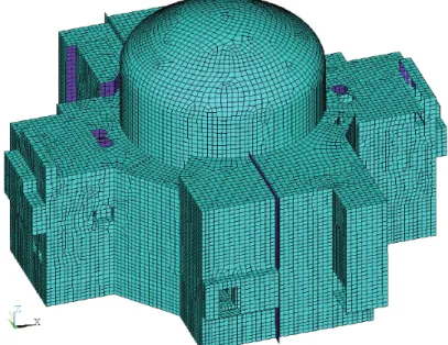
All the NI structures share a common foundation basemat. The NI is embedded approximately 11.6 m below the ground surface (Elevation -0.25 m). A detailed FE model of NI was first developed in ANSYS and then converted to MTR/SASSI for the SSI analysis. An isometric view of the FE model of the NI used in the SSI analysis is shown in Figure 1. The SSI model also includes the adjacent NAB. The NI structural model has over 450,000 degrees-of freedom (DOF). The total numbers of interaction nodes are approximately 45,000, 13,500 and 9,000 for DM, MSM, and SM, respectively. Eight soil cases covering the range of soft, medium, stiff to very stiff soil profiles were analyzed.
Because of the relatively large model size and number of interaction nodes, an advanced version of the SASSI program for HPC that runs on large computer clusters with shared memory is utilized for this study.
STRUCTURAL MODEL
Detailed FE Model
The US EPR™ NI consists of several buildings supported on a common basemat. These buildings include the RB, RCB, SB 1-4, and FB. Only structural elements relevant to assure a correct dynamic behavior of the NI buildings are considered.
Figure 1: NI Finite Element Model (NAB not shown)
The foundation level is at -11.85 m for all buildings because -11.85 m is the nominal elevation for the bottom of the basemat and is appropriate for the input of ground motions. Basemat, walls, and slabs are modeled with shell elements. Beam elements are used to model columns, the nuclear steam supply system (NSSS) and the polar crane. See Figure 1. Dynamic finite element models are developed for uncracked and cracked concrete where the cracked concrete model is selected in this study.
Soil Profile and Properties
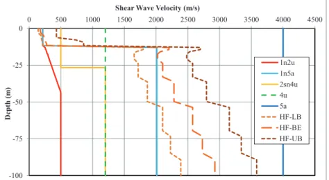
thicknesses matching the finite element grid of the NI basement walls. Soil case HF-UB is one of three high frequency (HF) cases considered in the US EPR™ design (see Figure 2). It consists of an 11.6 meter thick layer of medium stiff backfill over hard rock. The soil profile is subdivided into 36 sublayers.
Figure 2 : Soil Profiles for SSI analysis of the Nuclear Island Structures
Reference Motions
The reference motions used for the SSI analysis consist of one vertical and two horizontal components of each the EUR [3] Medium motion (EURM) and the HF motion. The motion is specified as full-soil column, free-field outcrop motion at the bottom of the NI basemat. The EURM motion has a maximum acceleration of 0.3g while the HF motion is anchored to 0.22g. The time histories have a time step of 0.005 seconds. The acceleration response spectra of these motions are shown in Figure 15 through Figure 26, labeled as reference motion.
SEISMIC ANALYSIS
SSI Analysis
The minimum passing frequency is calculated based on Vs/(5h) for DM, where Vs is the shear wave velocity and h is the largest element size of the soil layer under consideration. For the 2sn4u case, the shear wave transmissions are captured up to 56 Hz in the backfill and 56 Hz in the underlying hard rock. The frequency cut-off for the SSI model is set at 40 Hz. This is based on the characteristic of the input motion for this analysis case EURM, which does not have significant frequency content above 40 Hz. The analysis is performed for 57 computed frequencies with the intermediate frequency response values of the transfer functions obtained by interpolation. For the HF-UB case, the shear wave transmissions are captured up to 48 Hz in the backfill and over 100 Hz in the underlying hard rock. The frequency cut-off for the SSI model is set at 70 Hz. This is based on the characteristic of the input motion for this analysis case, which has significant frequency content up to 70 Hz. The analysis is performed for 87 computed frequencies.
Multiple key output locations in all buildings and elevations are output and examined. Those locations include vertically rigid and flexible positions in the buildings.
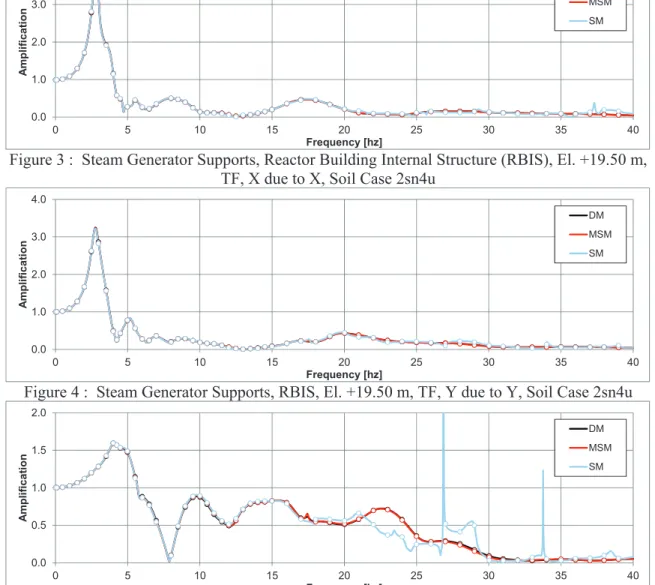
Transfer Functions
The transfer functions corresponding to the input motion applied separately in the x-, y-, and z-directions were output and examined. The results in the x-, y-, and z-direction at several key locations in the structure due to the x-, y-, and z-input motion, respectively, are shown in Figure 3 through Figure 14.
-100 -75 -50 -25 0
0 500 1000 1500 2000 2500 3000 3500 4000 4500
D
ep
th
(
m
)
Shear Wave Velocity (m/s)
In-Structure Response Spectra
The ISRS were calculated from the corresponding total acceleration time history responses in a given direction obtained by algebraically summing the co-directional acceleration time history output from separate analysis of the three directions of input motion. The computed 5%-damped ISRS at several key locations in the structure together with the corresponding spectrum of the reference foundation outcrop motion in the same direction are shown in Figure 15 through Figure 26.
Total Foundation Seismic Demand
The total dynamic soil reaction forces on the basement walls bearing against soil (sidewalls) were calculated using the dynamic force output option.
ANALYSIS RESULTS
Transfer Functions
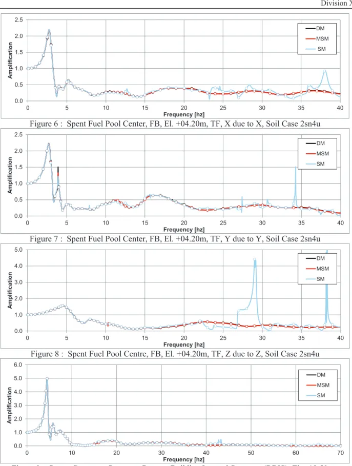
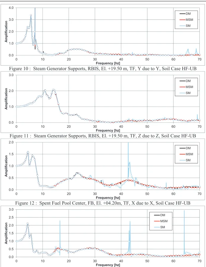
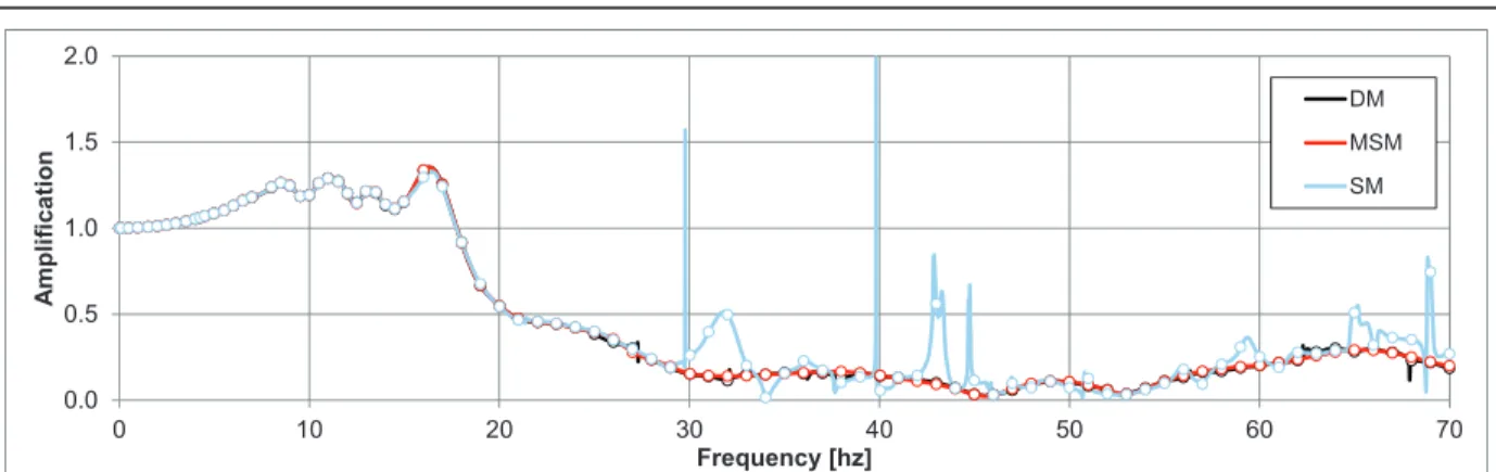
Transfer functions are shown in Figure 3 through Figure 14. MSM TFs match those from DM TFs for rigid and flexible locations. SM TFs start to deviate from DM TFs beyond approximately 20 Hz. The observed difference is the largest in the vertical direction (Z-Direction).
Figure 3 : Steam Generator Supports, Reactor Building Internal Structure (RBIS), El. +19.50 m, TF, X due to X, Soil Case 2sn4u
Figure 4 : Steam Generator Supports, RBIS, El. +19.50 m, TF, Y due to Y, Soil Case 2sn4u
Figure 5 : Steam Generator Supports, RBIS, El. +19.50 m, TF, Z due to Z, Soil Case 2sn4u
0.0 1.0 2.0 3.0 4.0
0 5 10 15 20 25 30 35 40
A
m
p
li
fi
c
a
ti
o
n
Frequency [hz]
DM
MSM
SM
0.0 1.0 2.0 3.0 4.0
0 5 10 15 20 25 30 35 40
A
m
p
li
fi
c
a
ti
o
n
Frequency [hz]
DM
MSM
SM
0.0 0.5 1.0 1.5 2.0
0 5 10 15 20 25 30 35 40
A
m
p
li
fi
c
a
ti
o
n
Frequency [hz]
DM
MSM
Figure 6 : Spent Fuel Pool Center, FB, El. +04.20m, TF, X due to X, Soil Case 2sn4u
Figure 7 : Spent Fuel Pool Center, FB, El. +04.20m, TF, Y due to Y, Soil Case 2sn4u
Figure 8 : Spent Fuel Pool Centre, FB, El. +04.20m, TF, Z due to Z, Soil Case 2sn4u
Figure 9 : Steam Generator Supports, Reactor Building Internal Structure (RBIS), El. +19.50 m, TF, X due to X, Soil Case HF-UB
0.0 0.5 1.0 1.5 2.0 2.5
0 5 10 15 20 25 30 35 40
A
m
p
li
fi
c
a
ti
o
n
Frequency [hz]
DM MSM SM
0.0 0.5 1.0 1.5 2.0 2.5
0 5 10 15 20 25 30 35 40
A
m
p
li
fi
c
a
ti
o
n
Frequency [hz]
DM MSM SM
0.0 1.0 2.0 3.0 4.0 5.0
0 5 10 15 20 25 30 35 40
A
m
p
li
fi
c
a
ti
o
n
Frequency [hz]
DM MSM SM
0.0 1.0 2.0 3.0 4.0 5.0 6.0
0 10 20 30 40 50 60 70
A
m
p
li
fi
c
a
ti
o
n
Frequency [hz]
Figure 10 : Steam Generator Supports, RBIS, El. +19.50 m, TF, Y due to Y, Soil Case HF-UB
Figure 11 : Steam Generator Supports, RBIS, El. +19.50 m, TF, Z due to Z, Soil Case HF-UB
Figure 12 : Spent Fuel Pool Center, FB, El. +04.20m, TF, X due to X, Soil Case HF-UB
Figure 13 : Spent Fuel Pool Center, FB, El. +04.20m, TF, Y due to Y, Soil Case HF-UB 0.0
1.0 2.0 3.0 4.0
0 10 20 30 40 50 60 70
A
m
p
li
fi
c
a
ti
o
n
Frequency [hz]
DM MSM SM
0.0 1.0 2.0 3.0
0 10 20 30 40 50 60 70
A
m
p
li
fi
c
a
ti
o
n
Frequency [hz]
DM MSM SM
0.0 0.5 1.0 1.5 2.0
0 10 20 30 40 50 60 70
A
m
p
li
fi
c
a
ti
o
n
Frequency [hz]
DM MSM SM
0.0 0.5 1.0 1.5 2.0 2.5 3.0
0 10 20 30 40 50 60 70
A
m
p
li
fi
c
a
ti
o
n
Frequency [hz]
Figure 14 : Spent Fuel Pool Center, FB, El. +04.20m, TF, Z due to Z, Soil Case HF-UB
In-Structure Response Spectra
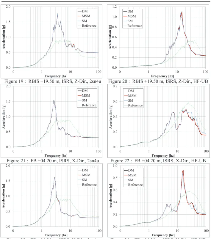
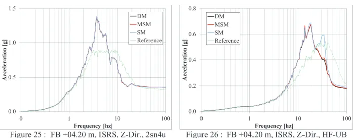
ISRS are presented in Figure 15 through Figure 26. The differences in TFs disappear in response spectra space for 2sn4u because of the limited input motion amplifications beyond 20Hz.
Figure 15 : RBIS +19.50 m, ISRS, X-Dir., 2sn4u Figure 16 : RBIS +19.50 m, ISRS, X-Dir., HF-UB
Figure 17 : RBIS +19.50 m, ISRS, Y-Dir., 2sn4u Figure 18 : RBIS +19.50 m, ISRS, Y-Dir., HF-UB 0.0
0.5 1.0 1.5 2.0
0 10 20 30 40 50 60 70
A m p li fi c a ti o n Frequency [hz] DM MSM SM 0.0 0.5 1.0 1.5 2.0 2.5 3.0
0 1 10 100
A cc el er a ti o n [ g ] Frequency [hz] DM MSM SM Reference 0.0 0.2 0.4 0.6 0.8 1.0
0 1 10 100
A cc el er a ti o n [ g ] Frequency [hz] DM MSM SM Reference 0.0 0.5 1.0 1.5 2.0 2.5 3.0
0 1 10 100
A cc el er a ti o n [ g ] Frequency [hz] DM MSM SM Reference 0.0 0.2 0.4 0.6 0.8 1.0
0 1 10 100
Figure 19 : RBIS +19.50 m, ISRS, Z-Dir., 2sn4u Figure 20 : RBIS +19.50 m, ISRS, Z-Dir., HF-UB
Figure 21 : FB +04.20 m, ISRS, X-Dir., 2sn4u Figure 22 : FB +04.20 m, ISRS, X-Dir., HF-UB
Figure 23 : FB +04.20 m, ISRS, Y-Dir., 2sn4u Figure 24 : FB +04.20 m, ISRS, Y-Dir., HF-UB 0.0
0.5 1.0 1.5 2.0
0 1 10 100
A cc el er a ti o n [ g ] Frequency [hz] DM MSM SM Reference 0.0 0.2 0.4 0.6 0.8 1.0 1.2
0 1 10 100
A c ce le r a ti o n [ g ] Frequency [hz] DM MSM SM Reference 0.0 0.5 1.0 1.5 2.0
0 1 10 100
A cc el er a ti o n [ g ] Frequency [hz] DM MSM SM Reference 0.0 0.2 0.4 0.6 0.8
0 1 10 100
A cc el er a ti o n [ g ] Frequency [hz] DM MSM SM Reference 0.0 0.5 1.0 1.5 2.0
0 1 10 100
A cc el er a ti o n [ g ] Frequency [hz] DM MSM SM Reference 0.0 0.2 0.4 0.6 0.8 1.0
0 1 10 100
Figure 25 : FB +04.20 m, ISRS, Z-Dir., 2sn4u Figure 26 : FB +04.20 m, ISRS, Z-Dir., HF-UB
Total Foundation Seismic Demand
The maximum and minimum total dynamic soil reaction forces are shown in Table 1. The largest difference between MSM and DM, and SM and DM for soil case 2sn4u is -0.96% and -1.18%, respectively. For soil case HF-UB it is -3.99% and -6.07%, respectively.
Table 1 : Maximum and Minimum Total Dynamic Driving Force
Analysis Direction Max / DM MSM SM
[kN] [kN] Diff. to DM [%] [kN]
2sn4u Fx Max 1752558 1749999 -0.15 1743688 -0.51
Min -1492172 -1487887 -0.29 -1492052 -0.01
Fy Max 1393843 1380485 -0.96 1377402 -1.18
Min -1559474 -1556886 -0.17 -1550848 -0.55
Fz Max 1700321 1701690 0.08 1695472 -0.29
Min -1470186 -1471787 0.11 -1471762 0.11
HF-UB Fx Max 573393 586123 2.22 585798 2.16
Min -520717 -508966 -2.26 -510148 -2.03
Fy Max 411957 402390 -2.32 396882 -3.66
Min -512149 -503521 -1.68 -495884 -3.18
Fz Max 568816 546135 -3.99 534296 -6.07
Min -565186 -554259 -1.93 -562565 -0.46
The total dynamic soil reactions of MSM and SM match DM reactions quite well. 2sn4u has larger reaction forces than the HF-UB case and the largest difference in total reaction force is in the Y-Direction.
Figure 27 : Total Dynamic Reaction Force, Y-Direction, Soil Case 2sn4u 0.0
0.5 1.0 1.5
0 1 10 100
A
cc
el
er
a
ti
o
n
[
g
]
Frequency [hz]
DM MSM SM Reference
0.0 0.2 0.4 0.6 0.8
0 1 10 100
A
cc
el
er
a
ti
o
n
[
g
]
Frequency [hz]
DM MSM SM Reference
-1.6E+06 -8.0E+05 0.0E+00 8.0E+05 1.6E+06
0 5 10 15 20
T
o
ta
l
H
o
ri
z
o
n
ta
l
F
o
rc
e
,
F
y
[
k
N
]
Time [sec]
The soil reaction time history for 2sn4u is plotted for the Y-Direction only in Figure 27. It shows good agreement amongst the various methods.
SUMMARY AND CONCLUSION
A comparison of typical transfer functions calculated in the structure for two soil cases, 2sn4u and HF-UB, for cracked concrete in the NI using Direct, Modified Subtraction, and Subtraction Method is shown in this paper. Even though the transfer functions of SM show some departure from those of DM and MSM at frequencies above 20 Hz, the ZPAs, ISRS, and reactions of MSM and SM in general are in good agreement with those of the Direct Method for soil case 2sn4u. This is because the input motions do not have a lot of energy beyond 20 Hz for 2sn4u. Meaningful structural responses occur at lower frequencies where the various SSI methods are sufficiently accurate. Soil case 2sn4u with cracked concrete properties is selected because the differences between SM and DM are the greatest amongst all generic analysis cases, further reinforcing the conclusion that the differences amongst the SSI results do not have a significant impact on the design of the US EPR™ NI structures.
Soil case HF-UB is selected to show the effect of the different SSI methods on the structural response in the high frequency region. While major structural responses are similar for the various methods, there is some variation in the ISRS that becomes evident in the high frequency region for SM even though higher wave passage frequencies were considered in the analysis.
It is recognized that while results from the different modeling techniques are close, there are DM results that are higher than either MSM or SM. In general, MSM results provide a significant improvement over those from SM. Although SM and MSM may produce slightly unconservative results, they may be sufficiently accurate for the purposes of conceptual or preliminary design. Given the computational intensity and associated cost of DM, it is important to recognize when SM or MSM may be appropriate for use. Other modeling techniques like Extended MSM (EMSM) where additional vertical or horizontal layers of interaction nodes are introduced provide further improvements. However, from a cost-benefit standpoint MSM provides the most efficient solution for this structure.
The HPC version of SASSI pushes the envelope on the size limits of finite element models, and the ability to capture a much higher frequency of interest than previously possible. It was also successfully used for the COL NI model with approximately 55,000 interaction nodes (increase in interaction nodes due to addition of Access Building). However, for this structure and its finite representation DM results conclusively demonstrated that sufficiently accurate results can be obtained using MSM.
ACKNOWLEDGMENT
We would like to acknowledge SC-Solutions1 for their contributions to the SSI analysis of the US EPR™ NI, as well as for the development of the high performance computing SASSI code in cooperation with MTR & Associates2. The authors would also like to thank the many engineers at AREVA who contributed to this effort and, in particular, to Todd Oswald for his guidance and unwavering support during the US EPR™ licensing process.
1 SC-Solutions Inc., Sunnyvale, CA, U.S.A.
2 MTR & Associates Inc., Lafayette, CA, U.S.A.
REFERENCES
1. Mertz, G., Costantino, C., Houston, T., and Maham, A. (2011), “SASSI Subtraction Method Effects at Various DOE Projects,” Natural Phenomena Hazards Workshop, U.S. Department of Energy. 2. Lysmer, J., Tabatabaie, M., Tajirian, F., Vahdani, S. and Ostadan, F. (1981), “SASSI – A System for
Analysis of Soil-Structure Interaction,” Report No. UCB/GT/81-02, Geotechnical Engineering, Department of Civil Engineering, University of California, Berkeley.