ABSTRACT
ROBBINS, DANIELLE. Sensitivity Functions for Delay Differential Equation Models. (Under the direction of H.T. Banks.)
Delay differential equations are useful to model various biological, sociological, and physical processes in which there are hysteretic or memory effects. Nicholas Minorsky played a great role in establishing the use of these type of models for physical processes. From his work, physical processes like ship control systems are modeled using delay differential equations with delayed damping or delayed restoring force. G.E. Hutchinson also saw the importance of using delay systems to model ecological models. Hutchinson’s equation, also known as the delay-logistic equation, is used to model population growth of a species.
For these biological and physical processes modeled using delay differential equations there are generally associated data sets. This data is used to estimate parameters within the model to gain the best predictive model for the process. When performing estimation procedures, pa-rameter identifiability issues may occur resulting in unfavorable estimates. There also may not be enough data or repeated information in the data which will again produce unfavorable esti-mates. Sensitivity analysis improves the estimation process as traditional sensitivity functions can determine which parameters can be estimated and those that should be fixed. Generalized sensitivity functions will determine which regions in the data help estimate specific parameters. Thus using both type of sensitivity functions should lead to optimal parameter estimates.
Sensitivity Functions for Delay Differential Equation Models
by
Danielle Robbins
A dissertation submitted to the Graduate Faculty of North Carolina State University
in partial fulfillment of the requirements for the Degree of
Doctor of Philosophy
Biomathematics
Raleigh, North Carolina 2011
APPROVED BY:
Ralph Smith Hien Tran
Ronald Baynes H.T. Banks
DEDICATION
BIOGRAPHY
ACKNOWLEDGEMENTS
I first would like to thank Jesus because without Him none of this would have been possible. My faith has sustained and kept me throughout this crazy experience called graduate school. I would like to thank my advisor Dr. Banks for his help because he has been more than an advisor but also a great mathematical father and I am appreciative. I would also like to thank Karyn Sutton who helped me get to NC State and has been supportive through everything. My friend, colleague, and fellow Biomathematican Kathleen Holm, you have been my greatest ally through out this whole ordeal and I truly love you! Thank you to Lesa Denning for all that you do and the CRSC for all of your support.
To my family, without you this would not of happened. Thank you to my parents who have followed me throughout my life and done whatever you could to make sure that I would be happy and successful. Thank you for loving me even when I was a brat, lol. Thank you for being great role models and instilling within me the importance of education. Thank you to my grandparents for all your love and support, for the summers of indulging my every want and need, and disciplining me when necessary, I love Jarratt, and Hampton, Va., they are a part of me. Thank you to my aunts and uncles and your listening to my mother’s wishes every summer and giving me my workbooks to do. Thank you to Aunt Connie for making hands-on science experiments for me to do, and all the many history lessons. Thank you Aunt Rosie, Uncle T-man, and Aunt Miki, Ryan, Christian and Maya, when I moved back to the east coast your home was my home and it made school that much easier. Thank you for always listening and letting me be frank with my younger cousins. Thank you to Aunt BJ for your cards and loving emails and gifts, they were much appreciated! Thank you to Uncle Darrell and Aunt Karen for the many check-in calls, Aunt Sheila for your love and support over the years and for just being you. To Uncle Alfred and Aunt Gwen, and all of my great aunts and uncles, cousins etc. thank you for the love and support. Thank you to my brothers Dwaine, Darian, and Keith, I know I was annoying growing up but as we have gotten older you really have become great friends and great support. Thank you to my cousin, sister, bff, Shamel, girl what would I do without you????? God only knows we have been through many endeavors together and I am glad this one ends together too. To Mrs. Betty and the Green/Whiten family thanks for all your love and care throughout the years, you are my family.
To the Goodman’s and Jenkins’, thank you for your support and encouragement I grateful to have two other sets of parents! To my church families (Mt. Peace, Tanner Chapel, and Quinn Chapel), Thank You, Thank You, Thank You, you’ve been a home away from home for me, no matter where I go you are always with me.
TABLE OF CONTENTS
List of Tables . . . .viii
List of Figures . . . ix
Chapter 1 Introduction . . . 1
1.1 History of Delay Differential Equations . . . 1
1.2 Previous Works for Parameter Identification Problems and Sensitivity Analysis in DDE Models . . . 2
Chapter 2 Theoretical Framework . . . 14
2.1 The Basic Model . . . 14
2.2 Theoretical Foundations . . . 15
Chapter 3 Parameter Estimation and Sensitivity Functions . . . 36
3.1 Parameter Estimation . . . 36
3.1.1 Mathematical and Statistical Models . . . 36
3.1.2 Generalized Sensitivity Functions . . . 37
3.2 Example: Delay-Logistic Equation . . . 39
3.2.1 Traditional Sensitivity function for the Delay Equation . . . 40
Chapter 4 Approximation of Delay Equations . . . 43
4.1 Banks-Kappel Spline Approximation . . . 43
4.2 Banks-Kappel Splines for Hutchinson’s Equation . . . 43
4.3 Pseudocode for Implementation of Method . . . 47
4.4 Numerical Comparison of BK-Splines, DDE23, and Method of Steps . . . 50
Chapter 5 Numerical Examples . . . 69
5.1 Delay Logistic Equation . . . 69
5.2 Harmonic Oscillators with Delayed Damping . . . 75
5.2.1 Traditional Sensitivity . . . 76
5.3 Harmonic Oscillator with Delayed Restoring Force . . . 80
5.3.1 Traditional Sensitivity . . . 80
5.4 A Behavior Change Model . . . 85
Chapter 6 Improving the Inverse Problem . . . 89
6.1 A Generic Inverse Problem . . . 89
6.2 Example: Hutchinson’s Equation . . . 90
6.3 Summary . . . 92
Chapter 7 Final Remarks . . . 93
7.1 Research Conclusions . . . 93
References. . . 95
Appendix . . . 98
Appendix A Numerical Implementation . . . 99
LIST OF TABLES
Table 6.1 Parameter estimates for the delay from the 3 types of simulated data sets (even or enhanced or enhanced+) at noise levels nl of 1%,5%, and 10%, Standard Error (SE) estimates, and 95% Confidence Intervals (CI), when
τ =.1. . . 91 Table 6.2 Parameter estimates for the delay from the types of simulated data sets
(even or enhanced or enhanced+) at noise levels,nl, of 1%,5%,and 10%, Standard Error (SE) estimates, and 95% Confidence Intervals (CI), when
τ = 1. . . 92 Table 6.3 Parameter estimates for the delay from the types of simulated data sets
(even or enhanced or enhanced+) at noise levels,nl, of 1%,5%,and 10%, Standard Error (SE) estimates, and 95% Confidence Intervals (CI), when
LIST OF FIGURES
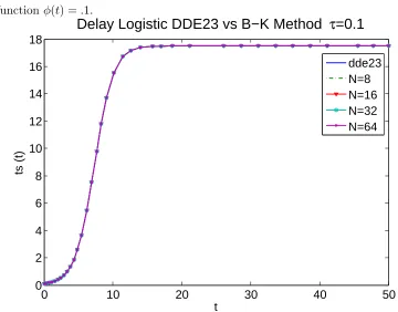
Figure 4.1 The numerical solution using the constant function φ(t) =.1 for τ =.1. . 51
Figure 4.2 The numerical solution using the constant function φ(t) =.1 for τ = 1. . . 52
Figure 4.3 The numerical solution using the constant function φ(t) =.1 for τ = 2πr. . 52
Figure 4.4 The initial condition φ(t) =sin(2τπt) for t∈[−τ,0], . . . 53
Figure 4.5 The numerical solution at τ =.1. . . 54
Figure 4.6 The initial condition φ(t) =sin(2τπt) for t∈[−τ,0]. . . 54
Figure 4.7 The numerical solution at τ = 1. . . 55
Figure 4.8 The initial condition φ(t) = sin(2πtτ ) for t ∈ [−τ,0], and the numerical solution at τ = 2πr. . . 55
Figure 4.9 The initial condition φ(t) = sin(2πtτ ) for t ∈ [−τ,0], and the numerical solution at τ = 2πr. . . 56
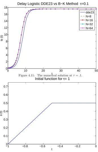
Figure 4.10 The initial conditionφ(t) =y(t) for t∈[−τ,0]. . . 57
Figure 4.11 The numerical solution atτ =.1. . . 58
Figure 4.12 The initial conditionφ(t) =y(t) for t∈[−τ,0]. . . 58
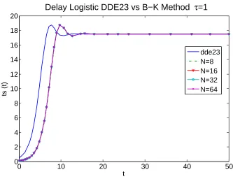
Figure 4.13 The numerical solution atτ = 1. . . 59
Figure 4.14 The initial conditionφ(t) =y(t) for t∈[−τ,0]. . . 59
Figure 4.15 The numerical solution atτ = 2πr. . . 60
Figure 4.16 The numerical solution using the constant functionφ(t) =.1 for τ = 2. . . 62
Figure 4.17 The numerical solution using the constant functionφ(t) =.1 for τ = 4. . . 62
Figure 4.18 The numerical solution using the constant functionφ(t) =.1 for τ = 8. . . 63
Figure 4.19 The numerical solution using the constant function φ(t) = sin(2πtτ ) for t∈[−τ,0] forτ = 2. . . 64
Figure 4.20 The numerical solution using the constant function φ(t) = sin(2πtτ ) for t∈[−τ,0] forτ = 4. . . 65
Figure 4.21 The numerical solution using the constant function φ(t) = sin(2πtτ ) for t∈[−τ,0] forτ = 8. . . 65
Figure 4.22 The numerical solution using the constant functionφ(t) =y(t) for τ = 2. 66 Figure 4.23 The numerical solution using the constant functionφ(t) =y(t) for τ = 4. 67 Figure 4.24 The numerical solution using the constant functionφ(t) =y(t) for τ = 8. 67 Figure 5.1 The numerical solution to the non-delay solution for x0 =.1, r=.7, K = 17.5 in (a). The numerical solution to the TSFs with respect to r, K, x0 for x0 = .1, r = .7, K = 17.5 for the non-delay solution in (b). The numerical solution to the GSFs with respect to r, K, x0 forx00=.1, r0 = .7, K0 = 17.5 for the non-delay solution in (c). . . 70
Figure 5.3 The numerical solution to the solution forφ=.1, x0=.1, r=.7, K = 17.5
and τ = 1 in (a). The numerical solution to the TSFs with respect to
r, K, x0, τ for x00 = .1, r0 = .7, K0 = 17.5 and τ0 = 1 in (b). The
nu-merical solution to the GSFs with respect to r, K, x0, τ forx00=.1, r0 =
.7, K0 = 17.5 and τ0= 1 in (c). . . 72
Figure 5.4 The numerical solution to the solution forφ=.1, x0=.1, r=.7, K = 17.5
and τ = 2πr in (a). The numerical solution to the TSFs with respect to
r, K, x0, τ for x00 = .1, r0 = .7, K0 = 17.5 and τ0 = 2πr in (b). The
nu-merical solution to the GSFs with respect to r, K, x0, τ forx00=.1, r0 =
.7, K0 = 17.5 and τ0= 2πr in (c). . . 73
Figure 5.5 The numerical solution to the Harmonic Oscillator K = 0, b=.5,τ = 1, and g(t) = 0 in (a). The numerical solution to the TSFs for the model with respect to K, b, τ at K0 = 0, b0 = .5, τ0 = 1, and g(t) = 0 in (b).
The numerical solution to the GSFs for the model with respect to K, b, τ
atK0 = 0, b0=.5,τ0= 1, andg(t) = 0 in (c). . . 77
Figure 5.6 The numerical solution to the Harmonic Oscillator K =.5, b= 2, τ = 1, and g(t) = 10 in (a). The numerical solution to the TSFs for the model with respect to K, b, τ at K0 = .5, b0 = 2, τ0 = 1, and g(t) = 10 in (b).
The numerical solution to the GSFs for the model with respect to K, b, τ
atK0 =.5, b0 = 2,τ0= 1, andg(t) = 10 in (c). . . 78
Figure 5.7 The numerical solution to the Harmonic Oscillator K =.5, b= 2, τ = 1, and g = g1 in (a). The numerical solution to the TSFs for the model
with respect to K, b, τ atK0 =.5, b0 = 2, τ0 = 1, andg=g1 in (b). The
numerical solution to the GSFs for the model with respect to K, b, τ at
K0 =.5, b0 = 2,τ0= 1, andg(t) =g1 in (c). . . 79
Figure 5.8 The numerical solution to the Harmonic Oscillator with no Restoring Force forK = 1,b= 0, andg(t) = 0. . . 82 Figure 5.9 The numerical solution to the Harmonic Oscillator with Delayed
Restor-ing Force when K = 5, b = .5, τ = 1, and g(t) = 10 in (a). The nu-merical solution to the TSFs for the model with respect to K, b, τ for
K0 = 5, b0 =.5, τ0 = 1, and g(t) = 10 in (b). The numerical solution to
the GSFs for the model with respect toK, b, τ forK0 = 5, b0=.5,τ0= 1,
and g(t) = 10 in (c). . . 83 Figure 5.10 The numerical solution to the Harmonic Oscillator with Delayed
Restor-ing Force when K = 5, b = .5, τ = 1, and g = g1 in (a). The
nu-merical solution to the TSFs for the model with respect to K, b, τ for
K0 = 5, b0=.5,τ0= 1, and g=g1 in (b). The numerical solution to the
GSFs for the model with respect to K, b, τ for K0 = 5, b0 =.5, τ0 = 1,
and g=g1 in (c). . . 84 Figure 5.11 The numerical solution to the alcohol behavior model whenτ = 1. . . 86 Figure 5.12 The numerical solution to the TSFs for dAdτ(t),dGdτ(t),and dDdτ(t) whenτ = 1
in (a). The numerical solution to the TSFs for dAdτ(t),dGdτ(t), and dDdτ(t) for
Figure 6.1 An example of a simulated data set with 10% noise and evenly spaced data points when τ =.1. . . 90 Figure 6.2 An example of a simulated data set with 10% noise and data points
con-centrated in the region of high information content for the delay parameter
Chapter 1
Introduction
1.1
History of Delay Differential Equations
Delay differential equations (DDEs) are used to model biological, physical, and sociological processes, as well as naturally occurring oscillatory systems. Minorsky in 1942 first introduces the idea of hysterodifferential equations in [38], using these type of equations to model self-excited oscillatory dynamical systems. He proposes the idea that some natural phenomena such as self-oscillations may be effected by the previous history of a motion or action, which describes a retarded dynamical system. A retarded dynamical system is a system that describes an action that has delayed time dependence [39]. Minorsky explains the importance of these systems due to their ability to model self-excitation within a control system. These physical systems are usually classified into systems with retarded damping given by
¨
x(t) +Kx˙(t−τ) +bx(t) =g(t), (1.1) and those with retarded restoring force described by
¨
oscillations in the solution [40]. This property of the DDE makes it very advantageous in mod-eling physical control systems. Minorsky also gives insight to the necessary use a non-linear DDE to model a system with self-excited oscillations, as a linear DDE is unable to capture all of the properties of the self-excitation. This is a result of the unstable conditions on the harmonic root [40]. Minorsky lays a foundation for modeling oscillatory phenomena in physical systems. From his research we are introduced to delayed restoring force and delayed damping DDE models which prove useful for modeling many physical and biological processes.
In 1948 Hutchinson developed a delay differential equation model, known as the delay logistic equation, to describe the dynamics of a circular causal system [32]. A causal system is a system where the output depends on the current and/or past input. A circular causal system is any causal system where changes to one part of the system effects another part of the system at a different rate so that the system does not go extinct. Parasite host interaction is an example of an ecological circular causal system since if a parasite can complete its life cycle without killing the host or drastically altering the growth of the host population, the host population will continue to exist [34, 32]. The delay in this model can represent various naturally occurring attributes of the process being modeled like the gestation period in a growing population, or the life cycle of a parasite. Hutchinson’s equation maybe used to model population growth, host population growth in the presence of a parasite, and various other biological and physical processes. From Minorsky and Hutchinson we learn early the importance of using DDE models.
1.2
Previous Works for Parameter Identification Problems and
Sensitivity Analysis in DDE Models
Usually for biological and physical processes modeled there are associated data sets from corre-sponding experiments. From these data sets and using the mathematical model that describes the process, we can perform the inverse problem to estimate the parameters within the model. In order to perform the inverse problem, the problem must be well-posed. The model param-eters must also be identifiable. In addition to these issues, a solution to the DDE model must exist.
for all the parameters including the delay to help with parameter estimation for DDE models. This analysis will involve computing TSFs and generalized sensitivity functions (GSFs). GSFs will give insight as to how sensitive the estimate is to the data and determine regions in the data of high information content. Thus from sensitivity analysis the TSFs will determine which parameters maybe fixed and the GSFs will determine when and where data should be collected, therefore improving the parameter estimation process.
A main issue when performing sensitivity analysis for DDE models occurs when deriving the equation for sensitivity with respect to the delay. For this particular sensitivity equation proving existence is not straight forward as the solution is dependent on the derivative of the previous history of the solution to the model, which we will see later is ˙x(t−τ). One main goal is to reformulate this sensitivity equation such that we can provide the theory to establish a well-posed problem. We begin by discussing previous work done on DDE parameter identification problems, followed by a discussion of previous work on sensitivity analysis for differential equation models. We compare and contrast the ideas presented in these works with our approach to the problem. We present theoretical and numerical results for multiple examples.
In the summarized works on parameter identification problems for DDE models, we learn that issues within parameter estimation leads to use of sensitivity equations to improve the estimation process. Also the theory presented in these works helps to direct our efforts for numerical computation of sensitivity functions. Next we present the works chronologically and summarize the results.
Banks, Burns, and Cliff in 1981 compute parameter identification problems for delay sys-tems [7]. Their research develops estimation algorithms for the parameters of the delay syssys-tems including estimation of the delay. They observed difficulty when estimating the delay since solu-tions of DDEs are not always differentiable with respect to the delays, which makes estimation methods such as least squares and maximum likelihood challenging. Banks, et al., also suggest the need for formal theory regarding the existence of sensitivity functions with respect to the delay. They formulate a class of estimation algorithms based on previous general approximation techniques for delay systems, and consider the following delay system identification problem
˙
x(t) = L(q)xt+B(α)u(t), t≥0, (1.3)
x(0) = η, x0 =φ , (η, φ)∈RN ×L2(−r,0;RN) (1.4) with outputy(t) =C(α)x(t) +D(α)u(t). Here the functionx,xt is defined such thatxt(θ) =
a compact convex parameter set Q⊂Rµ+ν by Q≡Ω× H, where
H={h= (r1, r2, . . . , rν)∈Rν|0≤ri≤ri+1, i= 1, . . . , ν−1}.
Then for any q= (α, h) ∈Q,L(q) is defined such that
L(q)φ=
ν X i=0
Ai(α)φ(−ri) + Z 0
−rν
K(α, θ)φ(θ)dθ.
Next, they introduce a more cohesive theoretical foundation for the identification problem of a delay system. Given the fundamental identification problem for the delay systems is linear, the problem can be reformulated in an abstract way such that its solution can be defined by a strongly continuous semigroup of linear operators. Thus equation (1.3)-(1.4) becomes
˙
z(t) = A(q)z(t) +B(α)u(t), t≥0 (1.5)
z(0) = (η, φ), (1.6)
y(t) = Cz(t) +D(α)u(t). (1.7) where (η, φ)∈Z ≡RN ×L
2(−r,0;RN), q ∈Qand the infinitesimal generator A(q) is defined such that
A(q)(φ(0), φ) = (L(q)φ,φ˙).
Then givent≥0,S(t;q) :Z →Z is defined such that
S(t;q)(η, φ) = (x(t;q), xt(q)),
whereS(t;q) is a strongly continuous semigroup. By defining a strongly continuous semigroup, from which a solution maybe obtained, a well-posed identification problem can be formulated. Banks et al., then prove approximation theorems, using semigroup theory, for the original model. As a result of the approximation theory established in their paper, computationally efficient identification algorithms are established. We will use the abstract formulation with our example to prove existence of a solution for the derived TSF equations with respect to the delay. We note that the original DDE may not have an existing solution if the initial history is not continuous over the time interval. For our DDE problem, the derived sensitivity function with respect to the delay, not only must the history of the solution,x(t−τ) be continuous, but the derivative of that history, ˙x(t−τ), must also be defined over the time interval.
abstract space. Next Brewer presents theory on Frechet derivatives for the solution of a linear abstract Cauchy problem [19]. The model observed is an autonomous linear abstract Cauchy problem
˙
z(t) = A(q)z(t) +u(t), (1.8)
z(0) = z0,
where z ∈ Z, a Banach space with norm || · ||, q ∈ Q, a normed linear space with norm | · |, and z0 is the initial condition. Brewer sets up criteria such that differentiability of the
solution with respect to a parameter may be established for both linear homogeneous and linear inhomogeneous equations. The operator in this paper, A(q), that defines the linear abstract Cauchy problem must be such that the parameterq may appear in unbounded terms. In previous work by Gibson and Clark [31], the differentiability results for this type of linear abstract Cauchy problem were obtained when the operator A(q) was represented as a linear combination of an operator independent of the parameter and a dependent bounded linear operator,A(q) =A+B(q). Brewer expands the class results in [31] by considering the operator,
A(q), to represent the parameter in an unbounded format. The operator will generate a strongly continuous semigroup, and using semigroup theory Brewer is able to prove the existence of
Frechet derivatives with respect to the parameters for the initial value problem (1.8). The solution to this problem via semigroups isS(t;q)z0 when u= 0. As a result of the existence of
the Frechet derivatives, he is able to carefully define sensitivity equations with respect to the parameters including the delay of the abstract system. Brewer applies his theory to a linear discrete delay system of the following format
˙
x(t) =a0x(t) +
n X k=1
akx(t−pk) +u(t)
to show the application of his result. His theory is formulated on the Banach space R×
L1(−p∗,0), but maybe be extended to the Hilbert spaceRm×Lν(−p∗,0) where m, ν ≥1. To use the results from this paper, there must be a general abstractlinear autonomous system dif-ferentiable with respect to the parameter. Since our problem is non-linear and non-autonomous, Brewer’s results are not readily extendable to our example.
point theory which are the methods we use to prove well-posedness for our problem. Banks considers the following system:
˙
x(t) = f(x(t), xt, x(t−τ1), . . . , x(t−τν)) +g(t), 0≤t≤T (1.9) x0 = φ,
where f : Z ×Rnν →
Rn, and Z = Rn×L2(−r,0;Rn). A nonlinear operator A is defined such that when reformulating (1.9) on Z the solution z(t;φ, g) = (x(t;φ, g), xt(φ, g)) will be a unique solution. Banks and Lamm [13] extend the definition of the operatorAto be dependent on both the parameter and time, and are able to show existence and uniqueness of a solution
z(t;φ, g) = (x(t;φ, g), xt(φ, g)) inZ. Although we employ the same techniques, Banks assumes a dissipative condition on the nonlinear operator for a class of functional differential equations to which our example does not fall. In this paper Banks’ main results show convergence of the approximating solutions using piecewise linear splines and proves well-posedness for a class of FDEs; however, the theory presented is not applicable to our class of FDE, which includes sensitivity equations for the delay parameter. The theory is not readily extendable for our class of FDEs because the right hand side of the derived sensitivity equation for derivative of the solution with respect to the delay is driven by the derivative of the history of the original solution. Thus we need different continuity requirements for our initial function.
In 1989, Brewer, Burns, and Cliff [20] carried out the parameter identification problem for an abstract Cauchy problem using quasilinearization. The linear abstract Cauchy problem is defined in (1.8). Given a solution to an abstract Cauchy problem is dependent upon a pa-rameter, and the Cauchy problem is defined by an unbounded parameter dependent evolution operator,A(q), their goal was to establish convergence of the gradient-based parameter estima-tion algorithm. The use of quasilinearizaestima-tion with parameter estimaestima-tion requires the derivative of the solution with respect to the parameter to be known (i.e., the gradient must exist). As a result Brewer, et al., show existence of Frechet derivatives with respect to the parameters, in-cluding the delay, using semigroup theory as applied to an autonomous linear delay differential equation. It is assumed that A(q) generates a strongly continuous semigroup S(t, q) on some Banach space with a norm,X. TheFrechet derivative with respect to the delay will exist based on the theory in this paper if the right hand side of the linear abstract Cauchy problem is not dependent on the derivative of the previous history of the original solution. In our problem, the derived sensitivity equation with respect to the delay, is dependent on the derivative of the previous history of the original solution and is a nonlinear delay differential equation model. Thus we are not readily able to apply the theory from this paper to our example.
the inverse problem on a DDE system and determine which methods best estimate parame-ters in the model. The following system of functional differential equations is the example for which the mathematical and statistical framework is based. The system of equations models the changes in an insect population due to insecticide and is given by,
dA dt(t) =
Z 5
−7
N(t+τ)m(τ)dτ−(dA(t) +pA(t)) dN
dt (t) = b(t)A(t)−(dN(t) +pN(t))N(t)− Z −5
−7
N(t+τ)m(τ)dt (1.10)
A(θ) = φ(θ), N(θ) =ψ(θ), θ∈[−7,0)
A(0) = A0, N(0) =N0.
Here A(t) is the number of adult insects, N(t) is the number of neonate insects, and m is a probability density kernel with specific assumed properties. To approximate the solution to this model, they use Banks-Kappel splines since the model may be reformulated into an abstract evolution equation. We will discuss the Banks-Kappel method in a later section. In this paper Banks et al., discuss the use and formulation of sensitivity equations with respect to the parameters and density kernel mbut do not present a formal proof on the existence of the
Frechet derivatives that define the sensitivity equations. They do however reference a formal proof presented in [11], which uses a theoretical framework presented in [16]. From Banks, Banks, and Joyner we observe the necessity to formulate and compute sensitivity functions with respect to the delay to aide parameter estimation because in their example, like in many other DDE models, the delay parameter in particular has the least amount of information given from the data and research.
Banks, Rehm, and Sutton [18] study inverse problems for nonlinear delays systems. They give a theoretical framework for the convergence of approximations for nonautonomous nonlin-ear DDE models. To establish this convergence, they begin by determining if solutions to the nonautonomous nonlinear DDE exist. To do this they reformulate their model
˙
x(t) = f(t, x(t), xt, x(t−τ1), . . . , x(t−τm), q) +f2(t), 0≤t≤T, (1.11)
x0 = φ, (1.12)
˙
z(t) = A(t;q)z(t) + (f2(t),0) (1.13)
z(0) = ξ= (φ(0), φ),
whereA(t;q) :D(A)⊂X →X is the nonlinear operator. They then determine if the abstract form has an existing solution. Banks et al.[18], suggests the existence of the solution can be established via fixed point theory and Picard iteration arguments. Existence and uniqueness for the solution of the approximation of (1.13) is established using the approach presented in [12]. Their main result ensures the convergence of solutions of the approximation to that of the original model. Banks, Rehm, and Sutton do not observe or formulate sensitivity equations; however, they do give insight to a theoretical framework for establishing existence and unique-ness for a DDE model. We use techniques presented here to establish well-posedunique-ness for our derived sensitivity equations with respect to the delay.
Next we describe previous work done on the computational aspects of sensitivity analysis for delay differential equations (DDEs). To be specific we discuss literature that uses sensitivity analysis on various DDE models [6, 17, 22] and the theory presented within these references. As we have previously mentioned, sensitivity analysis improves the parameter identification for process for DDE systems [5, 7, 13, 20], which use sensitivity functions in the identification process. From these works we discuss previous theoretical and computational tools and how there is a lack of proof of well-posedness for derived sensitivity equations with respect to the delay.
Baker and Rihan [17] show how to formally derive sensitivity equations for delay differential equation models, as well as the derivation of equations for the sensitivity of parameter estimates with respect to observations, what we know as GSFs. They consider a general system of delay differential equations such that p∈RL
˙
x(t, p) = f(t, x(t), x(t−τ), p), t≥0, (1.14)
x(t, p) = ψ(t, p), t≤0.
From this general model local sensitivity functions, ∂p∂x
i, are obtained by solving ∂x˙(t, p)
∂pi =
∂
∂pif(t, x(t), x(t−τ), p), t≥0, (1.15) ∂x(t, p)
∂pi
= 0.
ηj by first defining the cost functionalφ(p, η) φ(p, η) =X
i
[x(ti, p)−ηi].2 (1.16)
Next they differentiate the cost functional and obtain
∂ ∂pk
φ(p, η) = 2X
i
[x(ti, p)−ηi]∂x(ti, p)
∂pk
. (1.17)
If the cost function (1.16) is minimized ap= ˆp where ˆp≡pˆ(η), then (1.17) is equal to zero. So (1.17) becomes
X i
[x(ti,pˆ)−ηi]sk(ti,pˆ(η)) = 0, (1.18)
wheresk(ti, p) =∂x∂p(tik,p). Both sides are then differentiated with respect to ηi so N X i=1 Lp X l=1
[sk(ti,pˆ)sl(ti,pˆ) + [x(ti,pˆ)−η]rlk(ti,pˆ)]∂plˆ
∂ηj =sk(tj,pˆ). (1.19)
Given that x(ti,pˆ) is close to the observation ηi, [x(ti,pˆ)−η] = 0, (1.19) becomes N X i=1 Lp X l=1
[sk(ti,pˆ)sl(ti,pˆ)]∂plˆ
ηj ≈sk(tj,pˆ), (1.20)
which can be rewritten as
"N X
i=1
s(ti,pˆ)sT(ti,pˆ) #
∂pˆ
∂ηj ≈s(tj,pˆ). (1.21)
Thus
∂pˆ
ηj
≈
" N X i=1
s(ti,pˆ)sT(ti,pˆ) #−1
s(tj,pˆ).
Baker and Rihan also show that the sensitivity of the parameter estimates to observations (what we know as GSFs) maybe obtained by minimizing the previously defined objective func-tion φ(p) in the following way
∂
∂pφ(ˆp) = 2 N X j=1
whereχ(t,pˆ) is the sensitivity matrix.
Baker and Rihan also offer an outline of how to numerically compute both TSFs and GSFs for retarded delay differential equations and neutral delay differential equations. Baker and Rihan list issues that arise when doing parameter estimation in DDEs which includes difficulty in establishing existence of the derivative of the solution with respect to the parameters, as well as difficulty in establishing a well-posed problem for the derived sensitivity equations. The issues raised by Baker and Rihan are common when dealing with delay differential equations and we attempt to address and solve these issues within the current text.
Banks and Bortz [6] use sensitivity analysis to show how changes in parameters will effect the solutions of their delay differential equation model for HIV which has distributed delays. Their sensitivity equations are formulated from the following model:
˙
x(t) = L(x(t), xt) +f1(x(t)) +f2(t) for 0≤t≤tf (1.23)
(x(0), x0) = (φ(0), φ)∈R4×C(−r,0;R4),
where x(t) = (V, A, C, T),T which are the states used in the mathematical model for the HIV model, andL(η, φ) is a vector operator to account for the distributed delay. When deriving the sensitivity equations they obtain a system of DDEs, which are assumed to be well-posed. In their discussion of well-posedness for these sensitivity equations they assume the delay distributions are differentiable and parameterizable by a mean and standard deviation. In this paper they use theoretical steps presented in [5] to prove existence and uniqueness of the derived sensitivity equations (i.e., successive approximations, fixed point theory, Lipschitz continuity, etc.). While they are able to prove well-posedness for their particular class of sensitivity delay differential equations, their example does not have sufficient smoothness on the initial history functions, as it is assumed inC(−r,0;R4), such that the derivative of the history function will be defined over the time interval. Banks and Bortz also state that existence of the derived sensitivity function with respect to discrete delays can be established using the same manner of proof as their example; however, the arguments for this proof will be more tedious. From Banks and Bortz we gain more insight to the theoretical framework needed to prove a well-posed problem for derived sensitivity equations.
˙
x(t) = f(t, x(t), µ), t≥t0 (1.24)
x(t0) = x0,
where f : R+×X × M → X and M and X are complex Banach spaces. They establish
well-posedness for (1.24), and existence of Frechet derivatives with respect to the solutionx(t) and parameter(s)µ. As a result, there is a solution to the respective sensitivity equation
˙
y(t) = fx(t, x(t, t0, x0, µ), µ)y(t) +fµ(t, x(t, t0, x0, µ), µ), t≥t0 (1.25)
y(t0) = 0,
wherey(t) = ∂x∂µ(t). To prove existence of (1.25), they use fixed point, successive approximations, and Gronwall’s inequality theories. Banks and Nguyen apply their theoretical results to the DDE example for HIV dynamics, however they only display results for the the sensitivity with respect to the probability distribution for the delay and not a discrete delay which would require more details in the proof of existence. We follow closely the theoretical arguments within this paper and extend them for use in the proof of the existence of the Frechet derivative with respect to the delay for our examples.
Burns, Cliff, and Doughty [22] explain the use of continuous sensitivity equations for DDE models typical in biosciences, specifically for a model for Chlamydia Trachomatis. Their re-search focuses on parameter estimation techniques using sensitivity equations for DDE models specific to the biosciences. Parameter estimation for these typical models involves the inverse problem which uses sensitivity equations both theoretically and computationally. Burns et al., explore the parameter estimation problem for an ODE/PDE model of the cellular dynamics for Chlamydia Trachomatis which is then transformed into a simple DDE model to aid in the formulation of the continuous sensitivity functions. The following model describes the cel-lular changes between the retriculate body (RB) and extracelcel-lular elementary body (EB) in Chlamydia
d
dtRB(t) = a(t)RB(t), t1 < t < t3, (1.26) a(t) =
(
α, t1< t < t2,
α−β((t−t2)/(t3−t)), t2 < t < t3,
(1.27)
∂
∂tρ(t, s) = − ∂
∂sρ(t, s), t2 < t < t3, 0< s < r (1.28) ∂
where ρ(t, s) is the number of RB cells that transform to EB cells. This ODE/PDE can then be transformed to the following DDE
˙
x(t) = A0(q)x(t) +A1x(t−r) +Bv(t;q), 0< t < T, (1.30)
x(0) = ξ ∈Rn and x(s) =φ(s)∈L2(−r,0;RN), −r < s <0.
Once the ODE/PDE model for Chlamydia Trachomatis is transformed into the simple DDE, it is then transformed to a Cauchy Problem on the state spaceZ =RN ×L2(−r,0;RN)
dz(t;q, r)
dt = A(q, r)z(t;q, r) +Bv(t;q), (1.31)
z(0;q, r) = [ξ, φ0(·)]T ∈Z (1.32)
where
D(A(q, r)) ={[ξ, φ(·)]T :ξ∈RN, φ(·)∈H1(−r,0;RN), φ(0) =ξ} (1.33)
A(q, r)
" ξ φ(·)
#
=
"
A0(q)ξ+A1φ(−r)
φ0(·)
#
, (1.34)
and B =
" B
0
#
. (1.35)
Transformation to the Cauchy problem allows for use of specific numerical schemes to simulate the solution as established in previous literature [7, 12]. From the simple DDE (1.30) for the model they formulate the following continuous sensitivity equations
∂x˙(t;q, r)
∂q = A0(q)
∂x(t;q, r)
∂q + [
A0(q)
∂q ]x(t:q, r) +A1
∂x(t−r;q, r)
∂q +B
∂v(t;q)
∂q (1.36) ∂x˙(t;q, r)
∂r = A0(q)
∂x(t;q, r)
∂r +A1
∂x(t−r;q, r)
∂r −A1
∂x(t−r;q, r)
∂t (1.37)
which have a zero initial condition and initial function. Well-posedness is easily established for the sensitivity equations for the Chlamydia model with respect to parameters which are not the delay from semigroup theory for a linear autonomous operator (A0(q) +A1) as discussed in
respect to the delay. They only discuss ensuring that the initial past history of the solution to the original model is defined since it is a forcing term in the definition of this particular sensitivity equation, as shown in (1.37). Burns et al., give numerical results for estimated parameters of the Chlamydia model as well as sensitivities using SPLINE approximations coupled with MATLAB’s ODE 23. Burns et al., also use the Gauss-Newton procedure along with a step-size selection scheme to minimize the least squares cost functional. From this paper the authors give insight to numerical schemes for computing sensitivity functions for DDE models as well as parameter estimation techniques. They also highlight well-posedness issues for the sensitivity equation with respect to the delay.
Chapter 2
Theoretical Framework
2.1
The Basic Model
We begin with the following equation model which may describe a physical, sociological or biological system:
dx(t)
dt =G(x(t), x(t−τ), θ), t >0 (2.1) x(ξ) =
(
Φ(ξ), −τ ≤ξ <0
x0, ξ= 0
(2.2)
η(t) =h(x(t), x(t−τ), θ), t∈[0, T], (2.3) where x(t) ∈ Rn are vectors of state variables of the system, η(t) ∈ Rm is the vector of measurable or observable outputs, and θ∈Rp is the vector of parameters. It is assumed that G, andh in (2.1) and (2.3) are sufficiently smooth, in order to carry out the construction of the generalized sensitivity functions (GSFs). GSFs determine how sensitive the parameter estimate is to the observations or data.
When solving (2.1), we obtain x=x(t, θ), where t ∈[0, T], and
η(t) =f(t, θ), t∈[0, T],
and f is defined asf(t, θ) =h(x(t, θ), x(t−τ, θ), θ), whereh=h(x,x, θ˜ ) and ˜x=x(t−τ). We then can define the traditional sensitivity functions (TSFs) by
sk(t, θ) = ∂η ∂θk
(t, θ)∈RM, k= 1, . . . , p.
assumption thath is sufficiently smooth. We obtain the TSFs from the following equation:
d dt
∂x(t)
∂θ =
∂G ∂x
∂x ∂θ(t) +
∂G ∂x˜
∂x
∂θ(t−τ) + ∂G
∂θ(t), (2.4)
where the ∂θ∂ and dtd operators have been interchanged, due to the continuity assumptions made on Gand x, such that we have a delay differential equation (DDE) for the sensitivity function
∂x
∂θ. This DDE can be solved using MATLAB function dde23. The routine dde23 is an extended
ode23 solver using the method of steps to approximate the solution [43]. The TSFs are used in the definition for the GSF that will be discussed later.
2.2
Theoretical Foundations
We begin by establishing well-posedness for our model. Assuming that G(x(t), x(t−τ), θ) in (2.1) is continuous for t ≥0, a solution x(t, x0,Φ, τ, θ) for (2.1) satisfies the following integral
equation
x(t, x0,Φ, τ, θ) =
Φ(t), −τ ≤t <0;
x0 t= 0;
Rt
0 G(x(s, x0,Φ, τ, θ), x(s−τ, x0,Φ, τ, θ), θ)ds t >0.
To determine if a solution for the sensitivity equations exist, we must first determine if the solution for the delay differential equation defined in (2.1), exists, and is unique, and depends continuously on data using theory described in [16, 33, 34]. To show existence and uniqueness, we use Lemma 1, where the idea of successive approximations normally used with ordinary differential equations arguments are applied [16]. We define successive approximations in the following way for (2.1). Let k= 0,1,2, . . ., then
x0(t, x0,Φ, τ, θ) =
(
Φ(t) −τ ≤t <0
x0 t≥0.
xk+1(t, x0,Φ, τ, θ) =
Φ(t), −τ ≤t <0
x0, t= 0
Rt
0G(xk(s, x0,Φ, τ, θ), xk(s−τ, x0,Φ, τ, θ), θ)ds, t >0.
Lemma 1(Existence and Uniqueness of Solutions) LetG:Rn×Rn×Rp→Rnbe continuous and satisfy
|G(x1,x˜1, θ)−G(x2,x˜2, θ)| ≤C1|x1−x2|+C2|x˜1−x˜2| (2.7)
where Cj > 0 is a constant for j = 1,2, and assume that Φ ∈ L2(−τ,0;Rn). Then the suc-cessive approximations xk converge uniformly for t ∈[0, T] to a unique solution of the initial value problem (2.1) -(2.2) with the solution bounded on [0, T] and in fact, x ∈ H1(0, T;Rn). Moreover, if Φ∈H1,∞(−τ,0;
Rn), one has the solution satisfies x∈H1,∞(−τ, T;Rn).
Proof: Let I = [0, T] where t ∈ I and τ and θ are fixed. We let M > 0 such that |G(x,x, θ˜ )| ≤M for all t∈I. Thus
|x1(t, x0,Φ, τ, θ)−x0| ≤M tfort≥0.
To show that the successive approximations converge let
∆k(t, x0,Φ, τ, θ) =|xk+1(t, x0,Φ, τ, θ)−xk(t, x0,Φ, τ, θ)|.
Then,
∆k(t, x0,Φ, τ, θ) = |
Z t
0
G(xk(s), xk(s−τ), θ)−G(xk−1(s), xk−1(s−τ), θ)ds| ≤
Z t
0
|G(xk(s), xk(s−τ), θ)−G(xk−1(s), xk−1(s−τ), θ)|ds
≤
Z t
0
{C1|xk(s)−xk−1(s)|+C2|xk(s−τ)−xk−1(s−τ)|}ds, (2.8)
fort >0. Whent <0, ∆k(t, x0,Φ, τ, θ) = 0, sincexk(ξ) =xk−1(ξ) = Φ(ξ),forξ≤0.
Let ξ=s−τ; then the second term of (2.8) becomes
Z t
0
C2|xk(s−τ)−xk−1(s−τ)|ds=
Z t−τ
−τ
C2|xk(ξ)−xk−1(ξ)|dξ.
Then givent∈[0, T], and xk(ξ) =xk−1(ξ) forξ ≤0,
Z t−τ
−τ
C2|xk(ξ)−xk−1(ξ)|dξ≤
Z t
0
and thus
Z t
0
{C1|xk(s)−xk−1(s)|+C2|xk(s−τ)−xk−1(s−τ)|}ds
=
Z t
0
{C1|xk(s)−xk−1(s)|+C2|xk(s)−xk−1(s)|}ds
= (C1+C2)
Z t
0
|xk(s)−xk−1(s)|ds.
Let ˜C= (C1+C2), then
∆k(t, x0,Φ, τ, θ)≤C˜
Z t
0
∆k−1(s, x0,Φ, τ, θ)ds.
We claim that
∆k(t, x0,Φ, τ, θ)≤
MC˜ktk+1
(k+ 1)! , (2.9)
then for k= 0 and t∈I we have
∆0(t, x0,Φ, τ, θ) =|x1(t, x0,Φ, τ, θ)−x0| ≤M t.
By induction, we have
∆k+1(t, x0,Φ, τ, θ) ≤ C˜
Z t
0
∆k(s, x0,Φ, τ, θ)ds,
≤ C˜ Z t
0
MC˜ksk+1
(k+ 1)! ds ≤ MC˜
k+1tk+2
(k+ 2)! .
Therefore, we have that the inequality in (2.9) holds for all k and the series for P∞ k=0
∆k(t, x0,Φ, τ, θ) is dominated by the power series for M e
˜ Ct
˜
C . Thus using the comparison test,
the seriesP∞
k=0∆k(t, x0,Φ, τ, θ) converges uniformly on I. This implies that the series
x0+
∞
X k=0
converges uniformly and absolutely on I, and the partial sum
xn(t, x0,Φ, τ, θ) =x0+
n−1
X k=0
(xk+1(t, x0,Φ, τ, θ)−xk(t, x0,Φ, τ, θ))
converges uniformly to a continuous function x on interval I. Due to the existence ofx on I,
G(x(t), x(t−τ), θ) exists for t∈ I. Therefore given that xk(t, x0,Φ, τ, θ) converges uniformly
tox(t, x0,Φ, τ, θ), andx,x˜→G(x,x, θ˜ ) is continuous,
xk+1(t, x0,Φ, τ, θ) =x0+
Z t
0
G(xk(s, x0,Φ, τ, θ), xk(s−τ, x0,Φ, τ, θ), θ)ds
becomes in the limit as k→ ∞
x(t, x0,Φ, τ, θ) =x0+
Z t
0
G(x(s, x0,Φ, τ, θ), x(s−τ, x0,Φ, τ, θ), θ)ds.
Thereforex(t, x0,Φ, τ, θ) exists and satisfies (2.1). Moreover, it is easily seen that
x∈H1,∞(−τ,0;Rn) if Φ∈H1,∞(−τ,0;Rn).
To show uniqueness of the solution, we assume there exists two solutions to (2.1), x1(t) =
x1(t, x0,Φ, τ, θ), andx2(t) =x2(t, x0,Φ, τ, θ). We have
|x1(t)−x2(t)| = |
Z t
0
G(x1(s), x1(s−τ), θ)−G(x2(s), x2(s−τ), θ)ds|
≤
Z t
0
|G(x1(s), x1(s−τ), θ)−G(x2(s), x2(s−τ), θ)|ds
≤ C˜ Z t
0
|x1(s)−x2(s)|ds.
Then from Gronwall’s Inequality, it follows that
|x1(t, x0,Φ, τ, θ)−x2(t, x0,Φ, τ, θ)| ≤0e ˜
Ct= 0. (2.10)
Thusx1(t, x0,Φ, τ, θ) =x2(t, x0,Φ, τ, θ).
Lemma 2(Continuous Dependence of Solutions on Parameters)LetG:Rn×Rn×Rp→Rn, and given θ=θ0 letx(t, x0,Φ, τ, θ) be a solution of
˙
x(t) = G(x(t), x(t−τ), θ0), (2.11)
x(ξ) =
(
Φ(ξ), −τ ≤ξ <0
x0, ξ= 0
fort∈[0, T]. Assume that
lim
θ→θ0G(x,x, θ˜ ) =G(x,x, θ˜ 0), (2.12)
uniformly inx,x˜and for (x1,x˜1, θ),(x2,x˜2, θ)∈Rn×Rn×Rp, and assume that (2.7) is satisfied. Then the Initial Value Problem (IVP) (2.11)-(2.12) has a unique solution x(t, x0,Φ, τ, θ) that
satisfies
lim
θ→θ0x(t, x0,Φ, τ, θ) =x(t, x0,Φ, τ, θ0), t∈[0, T]. (2.13)
Proof: Existence and uniqueness of a solution on any interval [0, T] is provided by Lemma 1. To show continuous dependence of solutions onθ, lett∈[0, T], and x0 ∈Rn,Φ∈L2(−τ,0;Rn),
τ ∈Rbe fixed, we define z(t, θ, θ0) =x(t, θ)−x(t, θ0).
Then,
|z(t, θ, θ0)| = |x(t, θ)−x(t, θ0)|
≤
Z t
0
|G(x(s, θ), x(s−τ, θ), θ)−G(x(s, θ0), x(s−τ, θ0), θ0)|ds
=
Z t
0
{|G(x(s, θ), x(s−τ, θ), θ) +G(x(s, θ0), x(s−τ, θ0), θ)
−G(x(s, θ0), x(s−τ, θ0), θ)−G(x(s, θ0), x(s−τ, θ0), θ0)|}ds
≤
Z t
0
{|G(x(s, θ), x(s−τ, θ), θ)−G(x(s, θ0), x(s−τ, θ0), θ)|
+|G(x(s, θ0), x(s−τ, θ0), θ)−G(x(s, θ0), x(s−τ, θ0), θ0)|}ds
≤
Z t
0
˜
C|x(s, θ)−x(s, θ0)|ds+
Z t
0
{|G(x(s, θ0), x(s−τ, θ0), θ)
−G(x(s, θ0), x(s−τ, θ0), θ0)|}ds.
Let h(s, θ) = |G(x(t, θ0), x(s−τ, θ0), θ)−G(x(s, θ0), x(s−τ, θ0), θ0)|. Then h(s, θ) → 0
uniformly in s as θ→θ0 from the earlier described assumption in (2.13). Thus
|z(t, θ, θ0)| ≤
Z T
0
h(s, θ)ds+
Z t
0
˜
and with application of Gronwall’s inequality and the limit as θ→θ0 it follows that
lim
θ→θ0|z(t, θ, θ0)| ≤ θlim→θ0( Z T
0
h(s, θ)ds)eCt˜
= 0.
Therefore,
lim
θ→θ0x(t, x0,Φ, τ, θ) =x(t, x0,Φ, τ, θ0).
Now that we have established existence, uniqueness, and continuous dependence on θ for the solution to the model described in (2.1), to perform sensitivity analysis and obtain GSFs (defined in a later section) we must determine if (2.4) has a solution. We want to prove that
∂x(t)
∂θ exists and is given byy(t) that satisfies the system (2.15),(2.16). Lety(t) be the solution
of ˙
y(t) = Gx(x(t),x˜(t), θ)y(t) +Gx˜(x(t),x˜(t), θ)y(t−τ) +Gθ(x(t),x˜(t), θ), t >0(2.15)
y(t) = 0 −τ ≤t≤0. (2.16)
To show that the above differential equation has a solution given by the appropriate deriva-tive, we must prove that certain Frechet derivatives exists. Thus we must show
lim |h|→0
1
|h||G(x,x, θ˜ +h)−G(x,x, θ˜ )−A(h)| →0, where A is the operator of the Frechet derivative ofG atθ.
Lemma 3 Mean Value Theorem Let G:Rn×Rn×Rp → Rn and z = (x0,Φ) where Z is
Rn×L2(−τ,0;Rn).
(i) If Gx(x,x, θ˜ ) and Gx˜(x,x, θ˜ ) exists and are continuous for x ∈ Rn, then for x1, x2,x˜1,x˜2
∈Rn and θ∈
Rp,t≥0,
G(x1,x˜1, θ)−G(x2,x˜2, θ) =
Z 1 0
{Gx(sx1+ (1−s)x2, sx˜1+ (1−s)˜x2, θ)(x1−x2)
(ii) IfGθ(x,x, θ˜ ) exists and is continuous forx∈Rn, then forx,x˜∈Rnandθ1, θ2 ∈Rp,t≥0,
G(x,x, θ˜ 1)−G(x,x, θ˜ 2) =
Z 1
0
Gθ(x,x, sθ˜ 1+ (1−s)θ2)(θ1−θ2)ds.
(iii) Supposex(t, z, τ, θ) is a solution of (2.1), which is continuous in Rn and continuous and continuously differentiable for z ∈ Z, such that Dzx(t;·) ∈ L(Z,Rn), thus Dz = ∂z∂ is a bounded differential operator. Then forz1, z2∈Z, and a fixedτ ∈R,θ∈Rp, fort∈[0, T],
x(t, z1, τ, θ)−x(t, z2, τ, θ) =
Z 1
0
Dzx(t;sz1+ (1−s)z2)[z1−z2]ds.
Proof: We consider (i). Let
H1(s) =G(sx1+ (1−s)x2, sx˜1+ (1−s) ˜x2, θ), 0< s≤1
using the chain rule of Frechet derivative, we have
H10(s) = Gx(sx1+ (1−s)x2, sx˜1+ (1−s)˜x2, θ)(x1−x2)
+ Gx˜(sx1+ (1−s)x2, sx˜1+ (1−s)˜x2, θ)(˜x1−x˜2).
Then if we integrate H01(s) for s ∈ (0,1], we have H1(1)−H1(0) which is G(x1,x˜1, θ)−
G(x2,x˜2, θ), thus we have (i).
The proof of (ii) and (iii) are similar to the previous proof, thus we omit it.
Theorem 1 Suppose that G(x,x, θ˜ ) has continuous Frechet derivatives Gθ, Gx, Gx˜ such
that |Gx| ≤ M0,|G˜x| ≤M1, and |Gθ| ≤ M2. Then the Frechet derivative y1(t) = ∂x∂θ(t) ∈Rn×p exists and is the unique solution for
˙
y1(t) = Gx(x(t), x(t−τ), θ)y1(t) +Gx˜(x(t), x(t−τ), θ)y1(t−τ) +
Gθ(x(t), x(t−τ), θ), t >0 (2.17) y1(0) = 0 −τ ≤t <0.
m1(t, θ, h) =x(t, θ+h)−x(t, θ).
m1(t, θ, h) =
Z t
0
{G(x(s, θ+h), x(s−τ, θ+h), θ+h)−G(x(s, θ), x(s−τ, θ), θ)}ds
=
Z t
0
{G(x(s, θ+h), x(s−τ, θ+h), θ+h)−G(x(s, θ+h), x(s−τ, θ+h), θ) + G(x(s, θ+h), x(s−τ, θ+h), θ)−G(x(s, θ), x(s−τ, θ), θ)}ds. (2.18) Using Lemma 3, with Frechet differentiability then we can write (2.18) as
m1(t, θ, h) =
Z t
0
{
Gθ(x(s, θ+h), x(s−τ, θ+h), θ)[θ+h−θ] +w1(s, h)+ Gx(x(s, θ), x(s−τ, θ), θ)[x(s, θ+h)−x(s, θ)] +w2(s, m1(s, θ, h))
+ Gx˜(x(s, θ), x(s−τ, θ), θ)[x(s−τ, θ+h)−x(s−τ, θ)]
+ w2(s, m1(s−τ, θ, h))
}
ds,where w1(t, h) → 0 as h → 0, and w2(s, m1(s, θ, h)) → 0 as m1(s, θ, h) → 0. We define
b1(t, h) = w1|(ht,h| ) and b2(t, h) = w2|(m1t,m1(t,θ,h(t,θ,h)|)) so thatb1(t, h) → 0, and b2(t, h) → 0 as |h| → 0
and |m1(t, θ, h)| →0, respectively. Then for the Frechet derivative ∂x∂θ(t) to exist, as|h| →0 we
must argue
|m1(t, θ, h)−y1(t)h|
|h| →0, wherey1(t) is defined by (2.17). We argue that
|m1(t, θ, h)−y1(t)h|
|h| =
1 |h|
Z t
0
{|Gθ(x(s, θ+h), x(s−τ, θ+h), θ)[h] +w1(s, h)
+Gx(x(s, θ), x(s−τ, θ), θ)[m1(s, θ, h)] +w2(s, m1(s, θ, h))
+Gx˜(x(s, θ), x(s−τ, θ), θ)[m1(s−τ, θ, h)] +w2(s−τ, m1(s−τ, θ, h))
−h[Gx(x(s, θ), x(s−τ, θ), θ)y1(s) +Gx˜(x(s, θ), x(s−τ, θ), θ)y1(s−τ)
Hence,
|m1(t, θ, h)−y1(t)h|
|h|
≤
Z T
0
|Gθ(x(s, θ+h), x(s−τ, θ+h), θ)−Gθ(x(s, θ), x(s−τ, θ), θ)||h|
|h| ds
+
Z T
0
|Gx(x(s, θ), x(s−τ, θ), θ)||m1(s, θ, h)−y1(s)h|
|h| ds
+
Z T
0
|G˜x(x(s, θ), x(s−τ, θ), θ)||m1(s−τ, θ, h)−y(s−τ)h|
|h| ds
+
Z T
0
w1(s, h)
|h| +
Z T
0
w2(s, m1(s, θ, h))
|h| ds
+
Z T
0
w2(s−τ, m1(s−τ, θ, h))
|h| ds.
Then
|m1(t, θ, h)−y1(t)h|
|h|
≤
Z T
0
|Gθ(x(s, θ+h), x(s−τ, θ+h), θ)−Gθ(x(s, θ), x(s−τ, θ), θ)||h|
|h| ds
+
Z T
0
M0|m1(s, θ, h)−y1(s)h|
|h| ds+
Z T
0
M1|m1(s−τ, θ, h)−y1(s−τ)h|
|h| ds
+
Z T
0
b1(s, h)ds+
Z T
0
w2(s, m1(s, θ, h))
|h| ds+
Z T
0
w2(s−τ, m1(s−τ, θ, h))
|h| ds.
We need to show that w2(t,m1|h(|t,θ,h)) ≤Kw2|(m1t,m1(t,θ,h(t,θ,h)|)), so we consider
|m1(t, θ, h)| = |
Z T
0
{
Gθ(x(s, θ+h), x(s−τ, θ+h), θ)[h]+Gx(x(s, θ), x(s−τ, θ), θ)m1(s, θ, h)
+Gx˜(x(s, θ), x(s−τ, θ), θ)m1(s−τ, θ, h) +w1(s, h)
+w2(s, m1(s, θ, h)) +w2(s−τ, m1(s−τ, θ, h))ds
}
|≤
Z T
0
M2|h|ds+
Z T
0
M0|m1(s, θ, h)|ds+
Z T
0
M1|m1(s−τ, θ, h)|ds
+
Z T
0
|h|b1(s, h)ds+
Z T
0
b2(s, h)|m1(s, θ, h)|ds
+
Z T
0
Let ξ=s−τ, then
Z T
0
(b2(s−τ) +M1)|m1(s−τ, θ, h)|ds=
Z T−τ
−τ
(b2(ξ, h) +M1)|m1(ξ, θ, h)|dξ
≤
Z 0
−τ
(b2(ξ, h) +M1)|m1(ξ, θ, h)|dξ+
Z T−τ
0
(b2(ξ, h) +M1)|m1(ξ, θ, h)|dξ
≤0 +
Z T−τ
0
(b2(ξ, h) +M1)|m1(ξ, θ, h)|dξ≤
Z T
0
(b2(ξ, h) +M1)|m1(ξ, θ, h)|dξ
since for t∈[−τ,0], x(t, θ+h) =x(t, θ), so m1(t, θ, h) = 0. Using the change of variables, we
obtain the following:
|m1(t, θ, h)| ≤
Z T
0
M2|h|ds+
Z T
0
M0|m1(s, θ, h)|ds+
Z T
0
M1|m1(s, θ, h)|ds
+
Z T
0
b1(s, h)|h|ds+
Z T
0
b2(s, h)|m1(s, θ, h)|ds+
Z T
0
b2(s, h)|m1(s, θ, h)|ds
≤
Z T
0
(M2+b1(s, h))|h|ds+
Z T
0
(M0+M1+ 2b2(s, h))|m1(s, θ, h)|ds
≤ |h|K,
whereK = (M2+b1(s, h))e
Rt
0(M0+M1+2b2(s,h))ds when applying Gronwall’s inequality. Thus w2(t, m1(t, θ, h))
|h| ≤K
w2(t, m1(t, θ, h))
|m1(t, θ, h)|
.
Then
|m1(t, θ, h)−y1(t)h|
|h|
≤
Z T
0
|Gθ(x(s, θ+h), x(s−τ, θ+h), θ)−Gθ(x(s, θ), x(s−τ, θ), θ)||h|
|h| ds
+
Z T
0
M0|m1(s, θ, h)−y1(s)h|
|h| ds+
Z T
0
M1|m1(s−τ, θ, h)−y1(s−τ)h|
|h| ds
+
Z T
0
b1(s, h)ds+
Z T
0
Kw2(s, m1(s, θ, h))
|m1(s, θ, h)|
ds+
Z T
0
Kw2(s−τ, m1(s−τ, θ, h))
|m1(s−τ, θ, h)|
Then using the change of variables as shown earlier, we have that |m1(t, θ, h)−y1(t)h|
|h|
≤
Z T
0
|Gθ(x(s, θ+h), x(s−τ, θ+h), θ)−Gθ(x(s, θ), x(s−τ, θ), θ)||h|
|h| ds
+
Z T
0
M0|m1(s, θ, h)−y1(s)h|
|h| ds+
Z T
0
M1|m1(s, θ, h)−y1(s)h|
|h| ds
+
Z T
0
b1(s, h)ds+
Z T
0
Kb2(s, h)ds+
Z T
0
Kb2(s, h)ds
≤
Z T
0
|Gθ(x(s, θ+h), x(s−τ, θ+h), θ)−Gθ(x(s, θ), x(s−τ, θ), θ)||h|
|h| ds
+
Z T
0
(M0+M1)
|m1(s, θ, h)−y1(s)h|
|h| ds+
Z T
0
{b1(s, h) + 2Kb2(s, h)}ds.(2.19)
Since x(t, θ) is continuously dependent on θ for t ∈ [0, T], and Gθ is continuous, using Lemma 2, we have
lim |h|→0
|Gθ(x(s, θ+h), x(s−τ, θ+h))−Gθ(x(s, θ), x(s−τ, θ), θ)|= 0.
Thus
|Gθ(x(s, θ+h), x(s−τ, θ+h, θ), θ)−Gθ(x(s, θ), x(s−τ, θ), θ)| ≤b3(t, h),
whereb3(t, h)→0 as |h| →0. Then
|m1(t, θ, h)−y1(t)h|
|h| ≤
Z T
0
{b1(s, h) + 2Kb2(s, h) +b3(s, h)}ds
+
Z T
0
(M0+M1)
|m1(s, θ, h)−y1(s)h|
|h| ds.
Since as |h| → 0, b1(t, h), b2(t, h), and b3(t, h) → 0, and all functions are bounded, due to
dominated convergence we findK(h)→0 as h→0 where
K(h) =
Z T
0
{b1(s, h) + 2Kb2(s, h) +b3(s, h)}ds.
Thus with an application of Gronwall’s inequality we have
lim |h|→0
|m1(t, θ, h)−y1(t)h|
|h| ≤ |hlim|→0
{K(h)}eR0t(M0+M1)ds
Theorem 2 Suppose the function G(x,x, θ˜ ) of (2.1) has continuous Frechet derivatives
Gx(x,x, θ˜ ),G˜x(x,x, θ˜ ), with respect to x and ˜x, with
|Gx(x,x, θ˜ )| ≤M0, |G˜x(x,x, θ˜ )| ≤M1
for some constantsMj >0 forj = 0,1. Then the Frechet derivative y2(t) = ∂z∂x(t, z, θ) exists
withy2(t)∈ L(Z,Rn) (recall z= (x0,Φ), Z =Rn×L2(−τ,0;Rn)), and satisfies the equation ˙
y2(t)[h] = Gx(x(t), x(t−τ), θ)y2(t)[h] +G˜x(x(t), x(t−τ), θ)y2(t−τ)[h], t >0 (2.20)
y2(ξ) = I −τ ≤ξ≤0,
whereI ∈ L(Z,Rn) is the identity.
Proof: Using Lemma 1, we know that the differential equation (2.20) has a unique solution,
y2(t)[h]. For a fixedτ ∈R,θ∈Rp, andt∈[0, T], leth∈Z, andm2(t, z, h) =x(t, z+h)−x(t, z).
m2(t, z, h) =
Z t
0
{G(x(s, z+h), x(s−τ, z+h), θ)−G(x(s, z), x(s−τ, z), θ)}ds.
With the Frechet differentiability of G with respect to x ∈ Rn and for z ∈ L(Z,Rn), we have
m2(t, z, h) =
Z t
0
{
Gx(x(s, z), x(s−τ, z), θ)[x(s, z+h)−x(s, z)] +w3(s, m2(s, z, h))+Gx˜(x(s, z), x(s−τ, z), θ)[x(s−τ, z+h)−x(s−τ, z)] +w3(s, m2(s−τ, z, h))
}
dswhere
|w3(t, m2(t, z, h))|
|m2(t, z, h)|
→0 as|m2(t, z, h)|approaches zero. We define b4(t, h) as follows:
b4(t, h) =
|w3(t, m2(t, z, h))|
|m2(t, z, h)|
,
thenb4(t, h)→0 uniformly in t as|h| →0. To show thaty2(t) is a solution for (2.20), we must
show that
|m2(t, z, h)−y2(t)[h]|
|h| →0
By definition, |m2(t, z, h)−y2(t)[h]|
|h|
=|
Z t
0
{
Gx(x(s, z), x(s−τ, z), θ)[x(s, z+h)−x(s, z)] +w3(s, m2(s, z, h))|h|
+Gx˜(x(s, z), x(s−τ, z), θ)[x(s−τ, z+h)−x(s−τ, z)] +w3(m2(s−τ, z, h)) |h|
−{Gx(x(s, z), x(s−τ, z), θ)y2(s)[h] +Gx˜(x(s−τ, z), x(s−τ, z), θ)y2(s−τ)[h]}
|h|
}
ds|,then
|m2(t, z, h)−y2(t)[h]|
|h|
≤
Z t
0
{
|Gx(x(s, z), x(s−τ, z), θ)[x(s, z+h)−x(s, z)] +w3(s, m2(s, z, h))|h| |
+|G˜x(x(s, z), x(s−τ, z), θ)[x(s−τ, z+h)−x(s−τ, z)] +w3(s−τ, m2(s−τ, z, h))
|h| |
−|[Gx(x(s, z), x(s−τ, z), θ)y2(s)[h] +Gx˜(x(s−τ, z), x(s−τ, z), θ)y2(s−τ)[h]]
|h| |
}
ds.We want to show that
|w3(t, m2(t, z, h))|
|h| ≤K
|w3(t, m2(t, z, h))|
|m2(t, z, h)|
for some constantK >0. Thus we consider
|m2(t, z, h)|=
1 |h|
Z T
0
|Gx(x(s, z), x(s−τ, z), θ)[x(s, z+h−x(s, z)] +w3(s, m2(s, z, h))
+G˜x(x(s, z), x(s−τ, z), θ)[x(s−τ, z+h)−x(s−τ, z)] +w3(s, m2(s−τ, z, h))|ds
= 1 |h|
Z T
0
{
|Gx(x(s, z), x(s−τ, z), θ)[x(s, z+h)−x(s, z)] +w3(s−τ, m2(s, z, h))+Gx˜(x(s, z), x(s−τ, z), θ){
Z 1
0
Dzx(s−τ, r(z+h) + (1−r)z)[h]dr}
+w3(s−τ, m2(s−τ, z, h))|
}
ds.Thus with the assumptions that|Gx| ≤M0, and|Gx˜| ≤M1, the function|m2(t, z, h)|is bounded
by
Z T
0
M0|m2(s, z, h)|ds+
Z T
0
b4(s, h)|m2(s, z, h)|ds
+ Z T 0 M1 Z 1 0
{Dzx(s, r(z+h) + (1−r)z)[h]dr}ds+
Z T
0
b4(s−τ, h)|m2(s−τ, z, h)|ds.
We let ξ =s−τ and then we can write the previous as follows:
Z T
0
M0|m2(s, z, h)|ds+
Z T
0
b4(s, h)|m2(s, z, h)|ds
+ Z T 0 M1 Z 1 0
{Dzx(s, r(z+h) + (1−r)z)[h]dr}ds
+
Z 0
−τ
b4(ξ, h)|m2(ξ, z, h)|dξ+
Z T−τ
0
b4(ξ, h)|m2(ξ, z, h)|dξ.
When ξ ∈[−τ,0],m2(ξ, z, h) =I−I = 0, thus the function |m2(t, z, h)|is bounded by:
Z T
0
M0|m2(s, z, h)|ds+
Z T
0
b4(s, h)|m2(s, z, h)|ds
+ Z T 0 M1 Z 1 0
{Dzx(s, r(z+h) + (1−r)z)[h]dr}ds+ Z T−τ
0
b4(ξ, h)|m2(ξ, z, h)|dξ.
Then since Dz is a bounded operator, R01Dz x(s, r(z+h) + (1−r)z)[h]dr < hand
|m2(t, z, h)| ≤
Z T
0
M0|m2(s, z, h)|ds+
Z T
0
2b4(s, h)|m2(s, z, h)|ds
+
Z T
0
M1 h ds.
We apply Gronwall’s inequality to obtain
|m2(t, z, h)| ≤Kh
where K = M1T e
RT
0 (M0+2b4(s,h))ds and b4(t, h) → 0 uniformly in t as |h| → 0. Thus it follows
that
|w3(t, m2(t, z, h))|
|h| ≤K
|w3(t, m2(t, z, h))|
|m2(t, z, h)|
therefore
|w3(t, m2(t−τ, z, h))|
|h| ≤K
|w3(t, m2(t−τ, z, h))|
|m2(t, z, h)|
.
Thus we find
|m2(t, z, h)−y2(t)[h]|
|h| ≤
Z T
0
M0
|m2(s, z, h)−y2(s)[h]|
|h| ds+
Z T
0
K|w3(s, m2(s, z, h))|
|m2(s, z, h)|
ds
+
Z T
0
M1
|m2(s−τ, z, h)−y2(s−τ)[h]|
|h| ds+
Z T
0
K|w3(s−τ, m2(s−τ, z, h))|
|m2(s−τ, z, h)|
ds
≤
Z T
0
M0
|m2(s, z, h)−y2(s)[h]|
|h| ds
+
Z T
0
{K(b4(s, h) +b4(s−τ, h) +M1
|m2(s−τ, z, h)−y2(s−τ)[h]|
|h| }ds.
Letting ξ=s−τ in the last two integral terms, we have
|m(t, z, h)−y(t)[h]|
|h| ≤
Z T
0
M0
|m2(s, z, h)−y2(s)[h]|
|h| ds+
Z T
0
K(b4(s, h) +b4(ξ, h)ds
+
Z 0
−τ M1
|m2(ξ, z, h)−y2(ξ)[h]|
|h| dξ+
Z T−τ
0
M1
|m2(ξ, z, h)−y2(ξ)[h]|
|h| dξ.
When ξ ∈[−τ,0]
|m2(ξ, z, h)−y2(ξ)[h]|
|h| =
I−I−0·h
|h| , then
|m2(t, z, h)−y2(t)[h]|
|h| ≤
Z T
0
(M0+M1)
|m2(s, z, h)−y2(s)[h]|
|h| ds+
Z T
0
2K(b4(s, h))ds.
We apply Gronwall’s inequality and dominated convergence, and taking the limit as|h| →0, we conclude
lim |h|→0
|m2(t, z, h)−y2(t)[h]|
|h| ≤ |hlim|→0
{(
Z T
0
2K(b4(s, h)ds)e
Rt
0M0+M1ds}
= 0
Theorem 3 Suppose that G(x,x, θ˜ ) has continuous Frechet derivatives Gx, Gx˜ such that
|Gx| ≤M0, and|Gx˜| ≤M1 and suppose that the solutionx of (2.1)-(2.2) satisfies
x∈H1,∞(−τ, T;
Rn), for 0< τ < r for fixedr >0. Then the Frechet derivativey3(t) = ∂x∂τ(t) ∈
Rn exists and is the unique solution for
˙
y3(t) = Gx(x(t), x(t−τ), θ)y3(t) +Gx˜(x(t), x(t−τ), θ)[y3(t−τ)−x˙(t−τ)]
y3(ν) = 0, −τ ≤ν ≤0. (2.21)
Moreover, ∂x∂τ(t) is continuous inθ and, ifx∈C1(−τ, T;Rn) it is also continuous in τ.
Proof: We first reformulate (2.21) as a Cauchy problem on the state space Z1 = Rn×
L2(−r,0;Rn) with the norm |(ξ, φ)|2=|ξ|2+R−0r|φ(s)|
2ds.We may then consider solutions of
the system for τ0ssatisfying −r <−τ <0.
Let y3(t, τ) be a solution to (2.21) (we temporally suppress notation indicating the
depen-dence of solutions on θ). Then for t > 0 we define y3t(·) ∈ L2(−τ,0;Rn) by the past history
y3t(s, τ) =y3(t+s, τ), −τ < s <0. Ifz1(t, τ) = (y3(t, τ), y3t(·, τ))T, thenz1(t, τ) is a solution
to the abstract Cauchy problem
dz1(t)
dt = A(t, τ)z1(t, τ) (2.22)
z1(0, τ) = (0,0)T ∈Z1,
where D(A(t, τ)) ={(ξ, φ(·))T :ξ ∈
Rn, φ(·)∈H1(−τ,0;Rn), φ(0) =ξ}, and
A(t, τ)
" ξ φ(·)
#
=
"
Gx(x(t), x(t−τ), θ)ξ+Gx˜(x(t), x(t−τ), θ)[φ(−τ)−x˙(t−τ)]
φ0(·)
# .
Note that A(t, τ) is a vector affine operator on z1(t) = (y3(t), y3t(·))
T. Moreover, we note
that forx∈H1,∞(−τ, T;RN), we have existence of a unique solution to (2.21) or equivalently, (2.22). Thus we must argue that ∂x∂τ exists and also satisfies (2.21) (or (2.22)).
The proof follows the arguments for Theorem 1 with theGθterm replaced byGx˜{−x˙(t−τ)}.
That is, one defines the differences ˜m1(t, τ, h) =x(t, τ+h)−x(t, τ) and the difference quotients
|m˜1(t, τ, h)−y3(t, τ)h|
|h|
Theorem 1 provide the desired results for existence of ∂x∂τ(t) and that it satisfies (2.21).
We begin by defining the solution to (2.22) with successive approximations fork= 0,1,2, . . .,
z10(t;τ, θ) =
(
Φ(t) −τ ≤t <0
z10 t≥0.
(2.23)
zk1+1(t, x0,Φ, τ, θ) =
Φ(t), −τ ≤t <0
z10, t= 0
Rt
0A(s;τ, θ)z
k(s;τ, θ)ds, t >0.
(2.24)
Existence of the solution occurs when the successive approximations for z1(t;τ, θ) converge
ask→ ∞.
For t∈I = [0, T],τ ∈[−r,0], and a fixed θ,
|z1(t;τ, θ)−z10| = |
Z t
0
A(s;τ, θ)z10(s;τ, θ)ds| ≤
Z t
0
|
"
M0+M1
φ0(·)
#
(z10(s;τ, θ))|ds
≤ Q Z t
0
|z01(s;τ, θ)|ds
≤ Q Z t
0
|Nz|ds
≤ QNzt
fort≥0, whereQ≥
"
M0+M1
φ0(·)
#
, andz10is bounded byNz. Thus the first two approximations
forz1(t;τ, θ) converges.
Let ∆kz(t;τ, θ) =|z1k+1(t;τ, θ)−z1k(t;τ, θ)|, then
∆kz(t;τ, θ) = |
Z t
0
A(s;τ, θ)z1k+1(s;τ, θ)−A(s;τ, θ)z1k(s;τ, θ)ds| ≤
Z t
0
|A(s;τ, θ)(zk1(s;τ, θ)−z1k−1(s;τ, θ))|ds
≤ Q Z t
0
|(z1k(s;τ, θ)−z1k−1(s;τ, θ))|ds
≤ Q Z t
0
We claim that
∆kz(t;τ, θ)≤ MzQ
ktk+1
(k+ 1)! , (2.25)
where Mz=QNz. Then fork= 0 and t∈I
∆0z(t;τ, θ) =|z1(t;τ, θ)−z10| ≤Mzt
thus by induction we have
∆kz(t;τ, θ) ≤ Q Z t
0
∆kz−1(s;τ, θ)ds (2.26) ≤ Q
Z t
0
MzQksk+1
(k+ 1)! ds (2.27)
≤ MzQ
k+1tk+2
(k+ 2)! . (2.28)
Therefore (2.25) holds for all k, and the series forP∞
k=0∆kz(t;τ, θ) is dominated by the power
series for MzeQt
Q . Using the comparison test, the series P∞
k=0∆kz(t;τ, θ) converges uniformly on I. As a result, the series
z10+
∞
X k=0
(z1k+1(t;τ, θ)−zk1(t;τ, θ)) converges uniformly and absolutely on I, and the partial sum
z10+
n−1
X k=0
(z1k+1(t;τ, θ)−zk1(t;τ, θ))
converges uniformly to a continuous function z1 on interval I. z1 exists on I, and A(t;τ, θ)
exists for t∈I, then given that z1k(t;τ, θ) converges uniformly to z1(t;τ, θ), and t→A(t;τ, θ)
is continuous
z1k+1(t;τ, θ) =z10+
Z t
0
A(s;τ, θ)zk1(s;τ, θ)ds
becomes
z1(t;τ, θ) =z10+
Z t
0
A(s;τ, θ)z1(s;τ, θ)ds
![Figure 4.4:The initial condition φ(t) = sin( 2πtτ ) for t ∈ [−τ, 0],](https://thumb-us.123doks.com/thumbv2/123dok_us/1697274.1215013/66.612.135.472.243.520/figure-initial-condition-f-t-sin-ptt-t.webp)
![Figure 4.6:tThe initial condition φ(t) = sin( 2πtτ ) for t ∈ [−τ, 0].](https://thumb-us.123doks.com/thumbv2/123dok_us/1697274.1215013/67.612.135.477.58.653/figure-tthe-initial-condition-f-sin-ptt-t.webp)
![Figure 4.8:The initial condition φ(t) = sin( 2πtτ ) for t ∈ [−τ, 0], and the numerical solution atτ = π2r.](https://thumb-us.123doks.com/thumbv2/123dok_us/1697274.1215013/68.612.151.467.59.343/figure-initial-condition-sin-ptt-numerical-solution-att.webp)
![Figure 4.9:The initial condition φ(t) = sin( 2πtτ ) for t ∈ [−τ, 0], and the numerical solution atτ = π2r.](https://thumb-us.123doks.com/thumbv2/123dok_us/1697274.1215013/69.612.142.478.63.346/figure-initial-condition-sin-ptt-numerical-solution-att.webp)
![Figure 4.10:tThe initial condition φ(t) = y(t) for t ∈ [−τ, 0].](https://thumb-us.123doks.com/thumbv2/123dok_us/1697274.1215013/70.612.136.476.129.465/figure-tthe-initial-condition-f-t-y-t.webp)
![Figure 4.21:The numerical solution using the constant functionfor φ(t) = sin( 2πtτ ) for t ∈ [−τ, 0] τ = 8.](https://thumb-us.123doks.com/thumbv2/123dok_us/1697274.1215013/78.612.166.454.87.318/figure-numerical-solution-using-constant-functionfor-sin-ptt.webp)