The pattern of neutral molecular variation under the background selection model.

(1)

The Pattern of Neutral Molecular Variation Under

the Background Selection Model

D. Charlesworth, B. Charlesworth

and

M. T. Morgan’

Department of Ecology and Evolution, University of Chicago, Chicago, Illinois 60637-157? Manuscript received June 6, 1995

Accepted for publication September 1, 1995

ABSTRACT

Stochastic simulations of the infinite sites model were used to study the behavior of genetic diversity at a neutral locus in a genomic region without recombination, but subject to selection against deleterious alleles maintained by recurrent mutation (background selection). In large populations, the effect of background selection on the number of segregating sites approaches the effct on nucleotide site diversity, i.e., the reduction in genetic variability caused by background selection resembles that caused by a simple reduction in effective population size. We examined, by coalescence-based methods, the power of several tests for the departure from neutral expectation of the frequency spectra of alleles in samples from randomly mating populations (TAJIMA’S, Fu and LI’s, and WATTERSON’S tests). All of the tests have low power unless the selection against mutant alleles is extremely weak. In Drosophila, significant TAJIMA’S

tests are usually not obtained with empirical data sets from loci in genomic regions with restricted recombination frequencies and that exhibit low genetic diversity. This is consistent with the operation of background selection as opposed to selective sweeps. It remains to be decided whether background selection is sufficient to explain the observed extent of reduction in diversity in regions of restricted recombination.

S

ELECTION against deleterious alleles maintained by recurrent mutation (“background selection”) causes a reduction in the amount of genetic variability at linked neutral sites (CHARLESWORTH et al. 1993;

CHARLESWORTH 1994; HUDSON 1994; HUDSON and

-LAN

1994). This is because a new neutral variant can only remain in the population for a long period of time if it is maintained in gametes that are free of deleterious alleles, so that the effective population size in the presence of deleterious mutations is less than that based on the numbers of individuals in the population [see also FISHER (1930, Chapter 6 ) ; PECK (1994);

BARTON (1995)

3.

We previously showed that there can be large effects of background selection on genetic diversity in random-mating populations with no genetic recombination and in populations reproducing exclu- sively or largely by self-fertilization (CHARLESWORTH et al. 1993). These effects decrease rapidly with increasing recombination frequency or rate of outcrossing

(CHARLESWORTH et al. 1993; HUDSON 1994; HUDSON

and KAPLAN 1994). We concluded that observed reduc- tions in molecular variation in low-recombination genomic regions, such as the centromere-proximal regions of Drosophila autosomes (LANGLEY 1990; BEGUN and AQUADRO 1992; AQUADRO et al. 1994; W I T M A N and WAYNE 1994), or in highly selfing plant populations

Corresponding author: D. Charlesworth, Department of Ecology and Evolution, University of Chicago, 1101 E. 57th St., Chicago, IL 60637- 1573. E-mail: [email protected]

‘Present address: Department of Biology, McGill University, 1205 Ave. Dr. Penfield, Montreal, Quebec, Canada.

Genetics 141: 1619-1632 (December, 1995)

(HAMRICK and GODT 1990; SCHOEN and BROWN 1991; WOLFF 1991; FENSTER and RITLAND 1992; HANFSTING et

al. 1995) may be partly due to background selection against deleterious mutations.

Our previous simulation work on background selection employed a method that introduced neutral variants at a number of sites and followed their frequencies until either loss or fixation. This method enabled us to study the values of diversity measures relative to their neutral expectations for a range of parameter values, for instance with various recombination frequencies between the selected loci (CHARLESWORTH et al. 1993). With the population sizes studied previously (up to 6400 diploid individuals) we found that of the two measures of genetic diversity commonly used in studies of molecular variation (NEI 1987; KREITMAN 1991), the mean number of differences per nucleotide site between a pair of alleles at the neutral locus (x) was more strongly reduced than the number of segregating sites (s,)

.

This reflects the greater numbers of low-frequency variants compared with neutral expectation (CHARLESWORTH et al. 1993, Figure 2). Approximate analytical results suggested, however, that no difference in the effect of background selection on x and s, would be expected in very large populations (CHARLESWORTH et al. 1993).

(2)

1620 D. Charlesworth. B. Charlesworth and M. T. Morgan

BRAVERMAN et al. 1995; SIMONSEN et al. 1995). Such differences may provide a means of discriminating between alternative hypotheses to explain reduced genetic variability, such as background selection and hitchhiking. Our previous simulations were confined to small population sizes. Furthermore, they did not provide information on the properties of samples from populations and so did not permit us to assess the power of tests of the divergence of empirical data on allele frequency spectra from neutral expectation. We here present the results of simulations in which we examine both the diversity properties of very large randomly mating populations and the results of tests of divergence from neutrality using samples of realistic size.

SIMULATION METHODS

Two different programs were used to simulate the infinite sites model of molecular variation (KIMURA 1971) with the addition of selected loci in the genetic background. We assumed complete linkage between all loci, both those subject to selection against deleterious mutations (termed the selected loci in what follows) and also the neutral locus whose variation is of interest. Multilocus simulations thus need only keep track of the frequencies of gametes carrying different numbers of deleterious mutant alleles, and the genotypes at individual selected loci need not be followed. In both types of simulation, we assumed a randomly mating population of N diploid individuals. The loci subject to selection were assumed to be either wild type or mutant in state, with identical selection coefficients at each locus. In each generation, the sequence of events was mutation, reproduction, and selection. The numbers of new mutations per diploid individual that arise each generation were assumed to be Poisson distributed with mean U.

With large population size, homozygotes for deleterious mutations can be ignored, so that selection on diploid genotypes can be modeled by performing selection on haploid genotypes with fitnesses 1 for nonmutant and 1 - sh for mutant alleles, where s and h are, respectively, the selection and dominance coefficients for mutant alleles (CROW 1970). For the multilocus case, the fitnesses of haploid genotypes were usually calculated multiplicatively from these fitnesses, i.e., wI = (1 - sh)' is the fitness of the genotype with j heterozygous mutations. We also carried out some studies with synergistic epistasis among mutant effects on fitness (KIMURA and MARY- AMA 1966; CROW 1970; KONDRASHOV 1988; CHARLESWORTH 1990). In this case the quadratic-exponential fitness model was used, such that WJ = exp -j(a

+

' / 2 p ~ )

(CHARLESWORTH

1990). For both selection models, the equilibrium frequency distribution of gametes in each mutant class was assumed to be the stable state of the population during the course of a run. The vector of numbers of gametes in each class was found by multiplying the frequencies V;) by twice the number of diploid individuals in the population. This set of 2Nf; values was stored as an array of real numbers. With multiplicative fitness interactions among the selected loci, the relevant distribution of numbers of mutant alleles per gamete is Poisson with mean U/(2sh) (KIMURA and MARUYAMA 1966; CROW 1970). Most runs employed values of h and s of 0.1 and 0.2, ie., sh = 0.02, corresponding to a biologically reasonable infinite- population mean persistence time ( l / s h ) of 50 generations for a deleterious allele (CROW and SIMMONS 1983). With synergistic epistasis, the equilibrium distribution of numbers of mutations per gamete was found by iteration of the recursion

equations of K I M U R . ~ and MARUYAMA (1966) for the case of a sexual population with no recombination. Following CHARLESWORTH (1990) the selection coefficient against a heterozygous mutation in an equilibrium population with synergistic epistasis is given by the ratio of U to the equilibrium mean number of mutations per individual. This can be equated to sh in the multiplicative fitness model, enabling direct comparisons to be made between the two models.

Pseudo-sampling model: The first type of simulation was an infinite sites model with repeated introductions of variants at initially nonsegregating neutral loci, similar to the model studied previously (CHARLESWORTH et al. 1993). A pseudo- sampling scheme, similar to that of LI (1980) and KIMURA and TAKAHATA (1983) for single locus and two locus simulations, was used to increase the speed of the simulations and to enable us to examine the relative behavior of the two commonly used measures of genetic diversity, T and s,, in very large populations. A vector of frequencies of gametes carrying different numbers of deleterious mutations in each generation was generated from that in its parental generation by mutation, followed by selection and drift. Under suitable con- ditions, the first two processes, mutation and selection, can be treated deterministically, and only drift need be dealt with stochastically.

To simulate a pair of segregating alleles at a neutral locus, the program follows changes in the frequencies of gametes with the variant allele within each class characterized by its number of mutations at the selected loci. When a mutation at the neutral locus occurs, a single individual with the new variant is assumed to be present in one class, chosen randomly from the equilibrium distribution of the numbers of mutant alleles per gamete. Because there is no recombination and back-mutation is neglected, there is no movement from classes of genotypes with more selected mutations to classes with fewer mutations, but new individuals enter each class by mutation from classes with fewer mutations (so new neutral mutations occurring in genotypes without deleterious alleles will not necessarily remain in mutant-free genotypes), while selection against genotypes with mutations reduces the numbers of individuals in the class. The program contains expres- sions for the frequencies, p,, of gametes with i deleterious mutations and that carry the neutral variant. The transition probability from a gamete withj deleterious mutations to one with i mutations is the product of the marginal fitness w, of a gamete with j mutations (w7 = C, pLwIl) and the probability mk that such a genotype undergoes k = i - j mutations. The new frequency of gametes with i mutations that carry the variant is thus

F&wImk

a

p:

= ~

(1)

where is the population mean fitness (KIMURA and m u - YAMA 1966).

(3)

treated stochastically (CHARLESWORTH et al. 1993), the frequencies of loss and fixation, the times to loss and fixation, and the sum of the genetic diversity during the sojourn of a neutral variant in the population were followed for many replicate introductions of neutral mutations into these populations. The values of 7-r and s, relative to their values in the purely neutral cases were determined from these statistics as described by CHARLESWORTH et al. (1993).

For population sizes of 3200 and 6400 diploid individuals (the largest populations that we were previously able to run), but not with smaller population sizes, the results were very similar to those of simulations in which all stages of the life cycle were modeled stochastically (see Table 1 below). As our interest here is in large population sizes, however, it appears that the approximate simulation method is very satisfactory for our purposes.

Coalescence model: The second program generated results that allowed us to examine the standard genetic diversity measures (NEI 1987; KREITMAN 1991) and values of both TAJI-

MA'S and Fu and LI'S D statistics (TAJIMA 1989; FU and LI

1993) in samples of alleles at a single neutral locus subject to mutation according to the infinite sites model (KIMURA 1971). The diversity measures for such a sample are the mean number of nucleotide differences between pairwise combinations of sampled genes and the number of segregating sites in the sample (denoted here by k and S,, respectively, to distinguish them from the population values). In addition, the genes in the sample can be classed into different allelic categories according to the history of the neutral mutations that they carry, such that two genes can belong to the same allelic class only if they have identical genealogies and carry the same neutral mutations. The sample can then be characterized by its allelic configuration ( n l , %, . .

.

, n , ) , where m is the total number of different allelic classes in the sample, and n, is the number of times that the ith class is represented (EWENS 1972). A useful statistic for measuring the departure of the allele frequency spectrum from neutral expectation is provided by the sample homozygosity F = E, n , ' / ( z , nt)' (WATT- ERSON 1977, 1978). The greater abundance in the population of rare alleles under background selection compared with neutrality (CHARLESWORTH et al. 1993) means that the expectations of the sample values of the two kinds of D statistics should be smaller than in the neutral case, whereas F is expected to be larger.

To study these sample statistics, we generated genealogical trees of the neutral alleles whose sequence is examined, using the standard coalescence approach (HUDSON 1990), modified to take into account selection at the linked loci in the genetic background. The amounts of evolutionary change at the neutral locus are determined in the standard manner, using the times between nodes on the tree and a random process of assignment of neutral mutations to the branches (HUDSON

To make the method clear, we first describe the process for a neutral locus in a selectively neutral genetic background and then extend it to the case of linkage to selected loci in the genetic background. This process involves three stages, namely: (1) setting up a tree culminating in a sample of alleles at the neutral locus (with a preset sample size), including determining the generation at which each coalescent event occurred; (2) determining the number of mutations at the neutral locus between each node of the tree and its ancestral node; and (3) determining the genealogy of the sampled alleles at the neutral locus and the numbers of site differences between them. Stages 2 and 3 are the same whether there is or is not background selection, but the first stage differs.

Neutral case: A set of samples of neutral alleles was generated as described by HUDSON (1990). For each such sample,

1990).

we determined S,, the number of segregating sites in the sample, recorded how many of each allelic type are present, and used the matrix of numbers of site differences between allelic types to calculate the average number of pairwise differences ( k ) between the n ( n - 1)/2 different genes in the sample, including the zero differences between different alleles in the sample that are of the same allelic type. With real molecular data, the estimate of A is found from k = 7-r X the number of bases in the sequence studied. We used k and S, to calculate TAJIMA'S standardized D statistic (TAJIMA 1989),

DT. S,values were scaled by the quantity a, = E:=;' ( l / i ) . This facilitates comparisons with the k values, because both quantities have the same expectations under neutrality, M = 4Nv

(WATTEFSON 1975; TAJIMA 1989). Here, we will use 0 = S,/ al to denote the estimator of M obtained by equating the observed value of S, to its expectation.

We also computed the sum of the numbers of mutations in the external branches of the tree, as well as the total number of mutations in the tree. These two quantities were used to calculate Fu and LI'S standardized D statistic, 4 , using their method without an outgroup, as the phylogeny and branch lengths of the trees are, of course, completely known in our simulations (Fu and LI 1993). As discussed below, this implies that the method will be less powerful when applied to real data (for which branch lengths must be estimated from the data) than suggested by our results. Samples containing no variation at the neutral locus were not included in these calculations, as the values of the D statistics are zero for such samples. The program was run for 2000 replicate samples, and the values of the quantities just described were stored so that their distributions could be calculated.

Backgrand sebction case: The procedure for the case with natural selection against deleterious mutations in the genetic background is based on the same method, with the additional feature that the routine that generates the tree also keeps track of the numbers of mutations in the gametes. To do this, the program sets up a matrix of the probabilities that a gamete with i mutations in a given generation derives from an ances- tor in the preceding generation that has j mutations, similar to the approach used by HEY (1991) for generalizations of the classical coalescent process (see also HUDSON and KAPLAN 1994). We denote these probabilities by Q,. To calculate these values, taking into account selection on deleterious mutations, we use the selection models described above. As before, we assume that the population is at equilibrium under mutation and selection, with fixed frequencies of genotypes with different numbers of deleterious mutations.

Given a vector of frequencies,J, of gametes having different numbers of mutations, the transition matrix to the next generation is readily calculated, using similar logic to that leading to Equation 1. If m,, is the probability that a gamete experiences k = i - j mutations, the probability that a gamete with j mutations will produce a descendant gamete with i mutations ( i 2 J ] is

p ,

=

fm

-

W

where i 2 j . By BAYES' theorem, the probability that a gamete

with i mutations derives from a gamete with j mutations is

I

Once the program has been initialized by calculating the

(4)

1622 D. Charlesworth, B. Charlesworth and M. T. Morgan

TABLE 1

Results of pseudo-sampling simulations of large random-mating populations with no recombmation for various mutation rates to deleterious alleles

Observed mean Expected fixation time Observed values relative to neutral

times to time to expectation ( t S E )

loss Corrected for

Population size, N Loss Fixation (neutral) Neutral selected loci 7-r .%I

U = 0.1 ( f o = 0.082) 800 *800 1,600 1,600 3,200 *3,200 5,000 6,400 *6,400 10,000 100,000 200,000 500,000 1,000,000 5,000,000 1,600 3,200 *3,200 6,400 *6,400 10,000 100,000 200,000 500,000 1,600 3,200 6,400 10,000 25,000 50,000 100,000 200,000 500,000 1,000,000

U = 0.05 ( j ) = 0.287)

U = 0.025 (fo = 0.535)

8.34 9.75 8.42 9.18 8.58 9.21 8.66 8.74 9.38 8.08 8.45 8.01 7.13 6.33 4.33 10.10 10.56 11.32 11.01 11.52 11.29 11.49 11.15 10.641 12.14 12.97 13.47 13.96 14.75 15.30 15.39 17.03 15.69 14.23 428.1 1,167 753 78 1

1,222 1,288 1,631 2,176 2,182 3,468 32,427 73,404 157,691 326,705 1,653,190 2,002 3,764 3,764 7,122 7,122 10,762 115,578 227,118 521,656 3,648 7,463 12,351 22,975 53,565 114,398 217,948 454,255 1,250,360 2,119,820 14.67 14.67 16.06 16.06 17.50 17.50 18.39 18.91 18.91 19.81 24.41 25.80 27.63 29.02 32.24 16.06 17.51 17.51 18.90 18.90 19.80 24.41 25.80 27.63 16.09 17.52 18.91 19.80 21.65 23.02 24.41 25.80 27.63 29.02 3,066 3,066 6,131 6,131 12,618 12,618 19,716 25,491 25,491 40,000 400,000 800,000 2,000,000 4,000,000 20,000,000 6,155 12,683 12,683 25,366 25,366 40,000 400,000 800,000 2,000,000 6,236 12,750 25,501 39,845 100,000 200,000 400,000 800,000 2,000,000 4,000,000 393 393 645 645 1,177 1,177 1,760 2,234 2,234 3,280 32,966 65,791 164,301 328,461 1,641,837 1,881 3,751 3,751 7,385 7,385 11,566 114,720 229,310 573,099 3,420 6,907 13,732 21,410 53,583 107,084 214,085 428,270 1,070,553 2,141,106

0.1584 t 0.0034 0.30 t 0.022 0.1191 t 0.0028

0.1 1 t 0.007 0.1042 t 0.0027

0.09 -+ 0.006 0.0820 t 0.0030 0.0806 ? 0.0021 0.09 ? 0.005 0.0939 2 0.0026 0.0762 ? 0.0021 0.0824 2 0.0024 0.0778 t 0.0024 0.0774 ? 0.0022 0.0801 t 0.0024

0.3084

-+

0.0087 0.3091 ? 0.0090 0.33 t 0.018 0.2799 ? 0.0077

0.31 ? 0.038 0.31 17 t 0.0099 0.2739 t 0.0079 0.2834

-+

0.0080 0.2680 t 0.0075

0.5681 ? 0.0166 0.5903 ? 0.0174 0.5295 t 0.0146 0.5234 t 0.0154 0.5339 t 0.0178 0.4901 2 0.0211 0.5026 ? 0.0162 0.6735 ? 0.0649 0.5798 ? 0.0245 0.5374 ? 0.0220

0.5370 ? 0.0041 0.60 ? 0.008 0.4960 ? 0.0029

0.52 t 0.004 0.4670 ? 0.0023

0.48 ? 0.002 0.4448

-+

0.0026 0.4389 ? 0.0017 0.46 +- 0.003 0.3910 ? 0.0017 0.3337 2 0.0011 0.3012 t 0.0011 0.2507 ? 0.0010 0.2131 t 0.0009 0.1331 ? 0.0009

0.6143 t 0.0066 0.5928 t 0.0061 0.64 2 0.006 0.5687 t 0.0050

0.60 ? 0.012 0.5630 2 0.0058 0.4679 t 0.0039 0.4353 ? 0.0038 0.3855 ? 0.0034

0.7557 +- 0.0119 0.7495 ? 0.0113 0.7140 t 0.0093 0.7063 t 0.0092 0.6868 t 0.0097 0.6622 2 0.0107 0.6356 t 0.0082 0.7003 t 0.0030 0.5895 t 0.0105 0.5020 2 0.0050

Runs that were done without approximation, by full Monte Carlo simulation of the genotypes of the entire population, are

“Due to approximations involved in the simulations, these employed population sizes slightly less than the stated N values, indicated by asterisks.

and the expected fixation times were based on the actual sizes used in the simulations.

ous mutations are formed by sampling from thejdistribution. The first step in each generation (going back in time) is to obtain the number of mutations in the ancestral gamete of each gamete. These numbers are obtained by picking random Poisson deviates, using the Q,, probabilities as the expected values. Coalescence of alleles at the neutral locus can occur only between two gametes with the same number of deleterious mutations, so that each class of gamete with respect to the number of deleterious mutations is dealt with separately. For one such class, with k deleterious mutations, the program calculates the number L k of such nodes (gametes) present in the ancestry of the sample at the time point in question. The number of coalescence events that will occur in that mutational class is then found using a random binomial devi-

ate with parameters 1/(2Nf,) and &(Lk - l ) /2. When the population size N is large, we can, to a good approximation, neglect the possibility that the number of events within a given class is greater than one, although simultaneous coalescent events involving different gamete classes are permitted. The nodes that will undergo coalescence are picked randomly from those present in the given generation and mutational class, and the coalescence event(s) performed as described above.

(5)

Background Selection

jected to power analysis. The distributions of statistics in the samples without background selection were used to find the critical values such that deviations exceeding these values would occur at less than given defined levels of significance, for instance a frequency of 0.05 (one-sided). From the distributions of the statistics in samples with background selection operating, we could then determine the proportions of the samples of given size that had deviations in the direction of interest that were greater than the corresponding critical values for neutral samples of the same size.

In the case of WAITERSON'S homozygosity statistic, F, the distribution of sample E' values for a given number of allelic classes, m, can be computed directly (WATTERSON 1977, 1978), and a FORTRAN computer program was written to do this. This procedure for testing the departure of allele class configurations from neutrality was used rather than SLATKIN'S proposal that comparisons of samples of given size and number of alleles with the fraction expected under neutrality can be used for such a test for departure of a sample from neutrality (Su'rtuN 1994). SLATKIN'S method is not designed to test any particular type of departure from neutrality. In the present case, however, where one is interested in testing for an excess of rare alleles caused by hitchhiking or background selection, it seems preferable to make the more conventional comparison with the fraction of samples having F values in excess of certain critical values.

RESULTS

Infinite sites population model: The approximate analytical results generated previously suggested that, at least with low mutation rates, no difference in the effect of background selection on the two different measures of genetic diversity (7r and s,) would be expected in very large populations, although s, is affected less than 7r when population size is small

(CHARLESWORTH et al. 1993). Using the pseudo-sampling methods outlined above, we have now run simulations with much larger population sizes than before.

Table 1 shows some results assuming multiplicative fitnesses, for sh = 0.02 and with mutation rates of 0.1, 0.05, 0.025. The table shows the observed times to loss and fixation and the expected values based on standard neutral theory (KIMURA 1983). The expected fixation times are also shown after correction for the expected effect of background selection, obtained by multiplying the effective population size by the frequency of mutation-free gametes, f o = exp - U/ (2sh) (CHARLESWORTH

et al. 1993). The effects of background selection on the two measures of genetic diversity are also shown, in terms of their values relative to the neutral expectations for the same population sizes and mutation rates.

For population sizes above 3200, the table shows that, for all mutation rates, the mean time to fixation and 7r agree closely with those predicted theoretically, as was also found when populations were simulated in full in our previous study. But the mean time to loss and s,

are expected to converge very slowly on their asymptotic values, and even population sizes as high as lo6 are not expected to have reached their limiting values for these statistics (CHARLESWORTH et al. 1993). This slow conver-

"e Analytical

0.8

%

0.754

@"&

v)

O =

, 0.45 0.5 1

o3

l o 4 I

o5

1

o6

1 9

.

18i

/ t

17-

8

1 6 -

9

1 5 -

I-O 1 4 -

1 3 -

12- 3

-

1623

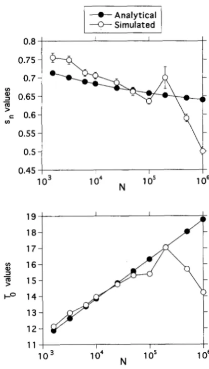
FIGURE 1.-Mean values of s, and time to loss ( T o ) from sets of simulations (0), compared with the analytical predicted values ( 0 ) for a Uvalue of 0.025 (sh = 0.02). SEs are shown for the s, values but not for the To values as they are too small to be visible.

gence can be seen in Table 1. For the higher mutation rates, it is is clear that even populations of over a million individuals have substantial departures of allele frequency distributions from those obtained under a purely neutral process. Figure 1 shows the relation between s, and N predicted by equation 10 of the Appen- dix of CHARLESWORTH et al. (1993) for the case of U = 0.025, together with the simulation results. The two agree quite well for N

>

3200, but the simulated values converge on

fo

considerably faster than predicted. A similar pattern is found for the mean time to loss.

With lower sh values, the s, values were larger for a given value of

fo

than shown in Table 1. For instance, with sh equal to 0.002, instead of 0.02, the values were 0.491 with U = 0.1, and 0.592 with U = 0.05. This is expected, since s, is an increasing function of the mean time to loss of gametes with deleterious mutations

(6)

1624 D. Charlesworth, B. Charlesworth and M. T. Morgan

TABLE 2

Mean values and standard errors of the sample statistics

Background selection U = 0.01, Background selection U = 0.1,

expectedf" = 0.779 expectedfo = 0.082

Sample size k 0 DT D,: k 0 DY. D,:

M = 1

20 0.719 0.753 -0.084 -0.147 0.086 0.093 -0.091 -0.185

0.014 0.012 0.023 0.024 0.004 0.004 0.051 0.053

50 0.564 0.731 -0.084 -0.185 0.086 0.094 -0.140 -0.202

0.013 0.01 1 0.027 0.030 0.004 0.003 0.038 0.042

100 0.740 0.788 -0.180 -0.396 0.091 0.107 -0.204 -0.483

0.015 0.010 0.023 0.027 0.004 0.003 0.036 0.044

20 7.85 7.84 -0.0900 -0.314 0.818 0.864 -0.170 -0.284

0.094 0.067 0.0'21 0.022 0.015 0.012 0.021 0.023

50 7.47 7.56 -0.132 -0.193 0.691 0.791 -0.293 -0.461

0.083 0.052 0.019 0.022 0.013 0.010 0.021 0.025

100 7.17 7.68 -0.290 -1.118 0.880 0.943 -0.163 -0.266

0.084 0.050 0.021 0.027 0.014 0.010 0.022 0.024

The table shows results from 2000 replicate runs with two different mutation rates for selected loci in the genetic background. Calculations of the D statistics include only samples that contained some genetic variation. M = 10

parture of the allele freqency spectrum from the neutral pattern if selection against deleterious alleles is weak than if it is strong, provided that the mutant alleles are maintained close to their deterministic equilibrium frequencies.

Coalescence model: The above results apply to the parameters of the population as a whole. It is possible that the effects of background selection could be too small to be easily detectable in samples from the population. Simulations based on the coalescent process were therefore done to ask two questions. First, can the effects of background selection on diversity measures be detected in samples of reasonable size (as opposed to the entire population)? Second, are significant values of test statistics for departures of allele frequency spectra from neutral expectation likely to be detected?

In the simulations, a mutation rate to deleterious mutations ( v ) of 0.1 or 0.01 per diploid genome per generation, multiplicative fitnesses with sh = 0.02, and a population size of N = 25,000 were assumed for most of the runs. From the results described above, this population size implies the existence of larger departures of frequency spectra from neutral expectation than is likely for the much larger effective sizes characteristic of most natural populations used for studies of DNA

variability. Two different M values were used, M = 1

and M = 10, representing the range from low to high values for empirical studies. The quantities of interest were generated as described in the previous section.

The distributions of the statistics of interest for samples of various numbers of genomes were calculated from runs both with and without background selection. In the absence of selection, the approximate simulation method used here produces results that are similar to

those obtained by TAJIMA (1989) and by Fu and LI (1993) for the same parameter values. The mean values of k and S, are close to M, as expected (WATTEMON 1975; TAJIMA 1989). The mean values of the D statistics in small samples are consistently negative, as found by

TAJIMA (1989) and Fu and LI (1993).

To make comparisons of the D statistics with samples simulated with background selection, neutral simulations with values of M approximately equal to the values expected in the presence of selection at linked loci were run ( i e . , M was discounted by a factor of f o , representing the expected reduction in nucleotide diversity due to background selection) (CHARLESWORTH et al. 1993).

As the true parameter values are not known for real samples, it is natural to compare empirical data with theoretical expectations that match the observed amounts of diversity. We should therefore make similar comparisons when we examine the power of statistical tests. Thus, for the higher mutation rate of U = 0.1, we compared the results with neutral runs with M reduced to -8% of the values with selection, i.e., for M = 10 we compared with neutral runs done with M = 0.8 (for n = 100) or M = 1 (for smaller samples with n = 20 or 50). The Mvalues were adjusted by using a lower mutation rate for the neutral runs.

(7)

Background Selection 1625

TABLE 3

Power tests for samples of various sizes for values of K and

8, with two M values, and two different mutation rates for selected loci in the genetic background

M = 1 M = 10

Sample size Pvalue k 8 k

e

u

= 0.01 20

50

100

u =

0.1 20 50 100 0.01 0.025 0.05 0.1 0.01 0.025 0.05 0.1 0.01 0.025 0.05 0.1 0.01 0.025 0.05 0.1 0.01 0.025 0.5 0.1 0.01 0.025 0.5 0.1 -

-

0.097 0.030 0.067 0.127 0.046 0.124 0.217

-

0.579 0.658 0.743 0.822 0.705 0.791 0.835

-

0.097 0.030 0.030 0.149 0.021 0.021 0.126

-

0.579 0.658 0.658 0.933 0.593 0.593 0.886

-

0.021 0.060 0.089 0.169 0.022 0.077 0.145 0.232 0.083 0.143 0.181 0.299 0.959 0.993 0.997 0.974 0.974 0.991 0.996

1 .000 0.963 0.977 0.994 0.998 0.009 0.054 0.119 0.235 0.046 0.123 0.216 0.331 0.063 0.096 0.202 0.289

1 .000 1 .000 1.000 1.000 1 .000 1 .000 1 .000 1 .000 1 .000 1 .000 1.000 1 .000

The table shows percentages of runs that yielded lower values than the critical points for the same M values and no background selection. Only samples that contained some genetic variation were included.

to detect the effect of background selection on genetic variability, even with samples as small as 20, at least with high M values. When Mfo is low because of strong background selection, there is a high probability that no diversity will be present in a sample. There is no great difference between the performance of k and 0

as diversity measures, despite the smaller variance of 6’ under neutrality (WATTERSON 1975; TAJIMA 1989). When a given critical point for the neutral case is a zero

(no genetic variability), it is impossible for background selection to produce a lower value, so the frequencies of these cases cannot be given and are indicated in the table by dashes.

These conclusions do not imply that the effect of background selection on the allele frequency spectrum will be easily detectable. Tables 3 and 4 show this clearly. The D statistics were affected in the qualitatively expected way, i.e., their means are all negative and larger in magnitude than in the comparable neutral cases. However, when we compare the distributions of the

D statistics with the results of neutral simulations with

TABLE 4

Power tests for samples of various sizes for TAJIMA’S and FU and LI’S statistics (DT and DF, respectively)

u

= 0.01

u=

0.1

Sample size Pvalue DT

4

07.

9

20 0.01 0.018 0.015 0.009 0.005

0.025 0.037 0.048 0.019 0.032

0.05 0.082 0.070 0.051 0.074

0.1 0.138 0.117 0.130 0.101 50 0.01 0.015 0.009 0.012 0.008

0.025 0.028 0.018 0.035 0.052

0.05 0.058 0.059 0.078 0.091

0.1 0.113 0.128 0.160 0.157

100 0.01 0.044 0.092 0.043 0.068

0.025 0.082 0.112 0.081 0.139

0.05 0.116 0.289 0.135 0.217

0.1 0.186 0.400 0.230 0.327

The table shows percentages of runs with M = 10 that yielded samples with variation that gave values than more extreme than the critical points for the case of no background selection. Only samples that contained some genetic variation were included. For the lower U values, comparisons were made with neutral runs with M = 8. For the higher V , comparisons were made with neutral runs with M = 1, which is close to the value of 0.8 expected under background selection with this mutation rate.

matching levels of diversity, their power to detect departures from neutrality in samples appears very limited (Table 4), even when the allele frequency spectrum in the population is strongly affected (Table 3). Even in sets of samples that exhibited extreme effects on the distributions of the diversity measures (e.g., the case of strong background selection with U = 0.1 and high

M, see Table 3) and with samples as large as 100, the proportion of samples that yielded test values more extreme than the critical points in the matched comparisons was less than three times as high as for the samples sets from neutral runs. The standard errors of the statistics for many of these cases were often lower than for the corresponding neutral cases, indicating that the shape of the distributions is changed by background selection, such that tails of the distributions are less extreme than with neutrality. Such an effect clearly means that comparisons with the critical points from the distributions obtained by neutral simulations may not be of much value in testing for the presence of background selection.

Table 4 shows only the samples generated with high Mvalues, because if significant effects on the frequency spectra are undetectable with such samples, it is impossible for samples with lower diversity to yield detectable effects, even if they are very large. This was borne out by runs with M = 1 with the higher mutation rate used in Tables 2 and 5, and with n = 100. For background selection with U = 0.1, significant values of both TAJI-

(8)

TABLE 5

Results of WAITERSON’S tests with background selection

assuming a mutation rate, 17, of 0.1

Fraction of samples with Fvalues greater than the critical point

M = 10 M = 10 M = 100

No. of alleles n = 50 n = 100 n = 100

2 205 83 3

0.3951 0.4458

3 387 175 7

0.1344 0.1543

-

4 459

5 414

6 254

7 142

0.1242 0.1

0.1377 0.1

0.1220 0.1

0.1761 0.1

Overall distribution

341 19

584 0.3158

362 19

492 0.2125

39 1 137

38 1 0.1971 299 216

505 0.1528

1861 1651 462

0.1628 0.1641 0.1818

Results are from 2000 samples of size n = 50 or 100 with various Mvalues. The results are shown for the P = 0.05 level only, for each sample constitution with respect to the number of alleles given at the top of each column of frequencies. Cases when the number of samples with a given number of alleles was too low to perform the test are indicated by-. The results when all allele numbers were combined are also shown.

quencies that were less than or equal to the expected frequencies under neutrality for all four critical points examined. This is because a large number of samples lack variability, so that the tests cannot be applied. For

U = 0.01, the frequencies were very slightly above the expected frequencies under neutrality (a maximum of 23% greater).

Runs with M

>

10 gave higher frequencies of samples outside the critical values. For instance, with M = 100 and a mutation rate of 0.1 in the genetic background, comparisons with critical values derived from neutral runs with M = 8 and samples of 100 alleles yielded 38% of samples beyond the 1 % point for FU and LI’S statistic, and 66% beyond the 5% point. The frequencies were lower for the TAJIMA test (10 and 23% for the 1 and 5% points, respectively). Very large M values in the absence of background selection were, however, needed to obtain this statistical power. With M = 20, the frequencies were similar to those with M = 10.

As described in METHODS, we also studied the perfor-

mance of WATTERSON’S homozygosity test (WATTERSON

1977, 1978). As the distribution of values of WATT- ERSON’S test depends on the number of alleles in the sample, we did the tests separately for the sets of samples with different numbers of alleles but also tabulated the results over all numbers of alleles for which reason-

ably large numbers of samples were obtained. Table 5 shows the results from samples with U = 0.1, for com- parison with the results given in Table 4 for the other two tests. With M = 10 and n = 50 or 100, the fractions of samples with higher values than the critical points are increased by a factor of two to three, compared with the neutral expectations. For instance, with n = 100, 15% of samples with seven alleles, and 18% of all samples, exceeded the 5% critical values. Table 5 shows that samples with small numbers of alleles are not very useful, as might be expected because the different critical points tend to be very similar to one another with small allele numbers. In general, even for samples with five or more allelic types, this test had low power, comparable with that of TAIIMA’S test, to detect the effect of background selection on the frequency spectrum but, unlike TAJIMA’S and FU and LI’S tests, there was no evident improvement in power in simulations with very high M values.

Efect of changes in the selection regime: It is important to consider the effect of the selection regime on the properties of samples from populations. The sh values used above were chosen because they correspond to the estimate of the harmonic mean effect of a heterozygous detrimental mutation on the fitness of Drosophila in nature (CROW and SIMMONS 1983). Potential effects in other species are, of course, also of interest, but at present few data are available either for estimating the relevant parameters or for testing predicted diversity values. In any species, it is likely that there is a wide distribution of selection coefficients around the mean, possibly with a long tail of rather weakly selected mutations (KEIGHT- LEY 1994). Since the simulations described above indicated that weaker selection tends to cause a larger devia- tion of the allele frequency spectrum from neutral expectation, there is thus a possibility that the results for large sh may underestimate the power of tests for deviations from neutrality.

We studied the effect of the magnitude of sh by similar analyses to those just described, assuming M = 10. We chose a low value of

j ,

(0.08) to produce strong background selection and studied samples of size 100,

(9)

Background Selection 1627

Tajima's D, Sample size 100

0.4 T-

O

0

Mutt, N = 25,000

Mult, N = 100,000

Mult, N = 500,000

Synergistic, N = 25,000

9

Y

0 0.005 0.01 0.015 0.02

hs value

Fu and

Li's

D,

Sample size 100

0.4 I I

Q

0

I " " / " " 0 0.005 0.01 0.015 0.02

hs value

FIGURE 2.-Fractions of TAJIMA'S Dand

Fu

and LI'S Dvalues that were significant at the 5% level, out of sets of 2000 samples of size 100 simulated with background selection. The mutation rate Uto deleterious alleles and the product shwere chosen such that the value offo was 0.08 in all cases. The D values were compared with their distributions in sets of neutral samples simulated with the same selection model and population size, but with M = 0.8 so that diversity was similar to that in the samples with background selection. Populations with N = 25,000, 100,000 and 500,000 were simulated under the assumption of multiplicative selection (denoted by Mult in the figure), and N = 25,000 was assumed for the runs with synergistic selection. The a and p values for synergistic selection were as follows: for hs

=

0.02, a was 0.08, was 0.032, and Uwas 0.1; for hs = 0.01, a was 0.004,

p

was 0.0016, and Uwas 0.05; for hs

=

0.005, a was 0.002, = 0.0008, and

U was 0.025.

As the results from the infinite sites model (see above) showed that the effect of background selection on the allele frequency spectrum tends to decrease with increasing population size, we also studied the effect of changing the population size. With a population of N

= 100,000 or 500,000, instead of 25,000 as above, the frequencies of significant results were lower for each sh value studied (Figure 2) . This conclusion was true even when both Nand sh were changed so as to preserve the same value of Nsh. With either Nsh = 50 ( N = 25,000 and sh = 0.002 us. N = 100,000 and sh = 0.0005) or Nsh = 500 ( N = 25,000 and sh = 0.02 us. N = 100,000

and sh = 0.005), the frequency of significant tests was lower with the lower selection, showing that the effect of sh was more important than that of population size. There has been much discussion of the evolutionary role of synergistic fitness interactions among deleteri-

ous mutations (KIMURA and MARYAMA 1966; CROW

1970; KONDRASHOV 1988; CHARLESWORTH 1990). For

this reason, we have also studied samples generated assuming synergistic interactions between the loci under selection (see METHODS). For the three strengths of selection studied with synergism (equivalent to sh values of approximately 0.02, 0.01 and 0.0052), the frequencies of significant results were very similar to those for the comparable cases with multiplicative selection (Figure 2). This suggests that we can have confidence in the conclusions obtained by assuming multiplicative fitnesses.

DISCUSSION

Our results for the case of no recombination, using the ITO approximate method of stochastic simulation, confirm our earlier conclusion that background selection causes an excess of rare variants over neutral expectation in populations of small to moderate size, and show that the difference between the behavior of 7r and s, diminishes as population size becomes very large (Table 1 and Figure 1). Figure 1 shows that that the ratio of s, to the classical neutral values approaches its asymptotic value offo = 0.535 faster than expected from the analytical result. As the population size increases,

so that selection becomes more effective, the mean time to loss (which is the major influence on s,) is increas- ingly overestimated by the analytic approximation. This is not unexpected, since this formula ignores the possibility that a gamete carrying a single deleterious mutation acquires a further mutation (and so is selected against more strongly) before elimination from the population (CHARLESWORTH et ul. 1993).

(10)

1628 D. Charlesworth, B. Charlesworth and M. T. Morgan

pected intensity (although this may not be detectable in samples by tests such as TAJIMA’S and FU and LI’S tests; see below).

With samples of realistic sizes, the simulations of the coalescent process with selection show that the effect on the level of genetic diversity should be detectable (Table 3 ) . This is in accord with the only currently available data from Drosophila, which indicate reduced variability at the DNA level at loci in regions of reduced recombination (see below). The tests of departure from neutrality studied here offer (in principle) the possibility of determining whether observed instances of reduced genetic diversity could be explained by background selection. But significant departures of allele frequency spectra from expectations under neutrality (as assessed by the values of TAJIMA’S or Fu and LI’S statistics, or by Watterson’s test) are unlikely to be found under background selection with the “standard” sh

value of 0.02 that corresponds to the estimated harmonic mean selection coefficient against a heterozygous detrimental mutation in Drosophila (MUKAI 1964;

MUKAI et al. 1972; CROW and SIMMONS 1983). This re- mains true even when the true population size is small, so that the

x

and

8

values (relative to neutral expectation) for the population are expected to differ widely. This conclusion is based on our simulations employing populations of size 25,000. In real populations of Dro- sophila, which appear to have very large effective population sizes (KREITMAN 1983), it is even less likely that one will detect an effect. Even a fourfold increase in population size yields samples with much lower frequencies of statistically significant D values, for a given value of sh (see above). The low power of TAJIMA’S D

statistic for detecting the effect of background selection has also been noted by HUDSON and

-LAN

(1994).

A limitation of our results is that they are based on the unrealistic assumption of identical selection coefficients for all selected mutations. This restrictive assump tion enables us to use the technically very convenient coalescence method. It remains to be seen how our conclusions might be changed if samples were generated with mutations at the selected loci drawn from some biologically plausible distribution of heterozygous selection coefficients. Since, however, even selection one hundred times weaker than the current best estimate of the mean value yields only modest frequencies of significant test statistics if effective population size is large (Figure 2 ), our conclusion appears robust; reduction of genetic diversity due to background selection seems unlikely to be frequently associated with significant values of any of the test statistics examined here, in contrast to what is found with hitchhiking (see below).

A difficulty that is inherent in the nature of the empirical data is that strong effects of background selection, which are most likely to cause large departures of allele frequency spectra from neutral expectation, tend to result in a high frequency of samples with little or no

variability, so that the ability to test for such departures is very limited (see Table 3). Significant differences from the neutral expectation were seen with apprecia- ble frequency only when we modeled very high diversity

( M = 100) and strong background selection ( U = 0.1). In this set, FU and LI’S statistic yielded more than twice the frequency of significant results than TAJIMA’S test. A similar superiority of FU and LI’S test is also seen in many of the results given in detail in Table 4, though the difference is usually not as large. These findings suggest that TAJIMA’S test is not as good as Fu and LI’S test at detecting the effects of background selection. It

is important to note, however, that this comparison is based only on our simulations, in which the phyloge- netic trees are completely known. With real data sets, it is necessary to perform this test to construct trees from the data, or from other sources of information, so the error inherent in this process might outweigh this benefit. There is also no reason from our results alone to believe that FU and LI’S test must be superior as a test for other departures from neutrality, such as hitchhiking, for example. It is therefore probably best to use both tests on real data sets. Our results also sug-

gest that WATTERSON’S test is not appreciably better at detecting the effects of background selection than TAJIMA’S test (Tables 4 and 5).

As

WATTERSON’S test is considerably more troublesome to perform, it does not seem to be a satisfactory means of testing for the causes of lowered genetic diversity.

These results imply that data on very long sequences would be necessary to detect the effects of background selection on allele frequency spectra. A diversity value per nucleotide site of 0.005, a typical value for a gene in a freely recombining section of the D. melanogaster genome (LANGLEY 1990), is equivalent to a sequence of length M/0.005 or 20,000 bases for M = 100. Surveys of such large tracts are unlikely to be possible in studies that use sequencing as the only methodology. Methods such as single-strand conformation polymorphism, which can survey large tracts of DNA (e.g., AGUADE et

(11)

Background Selection

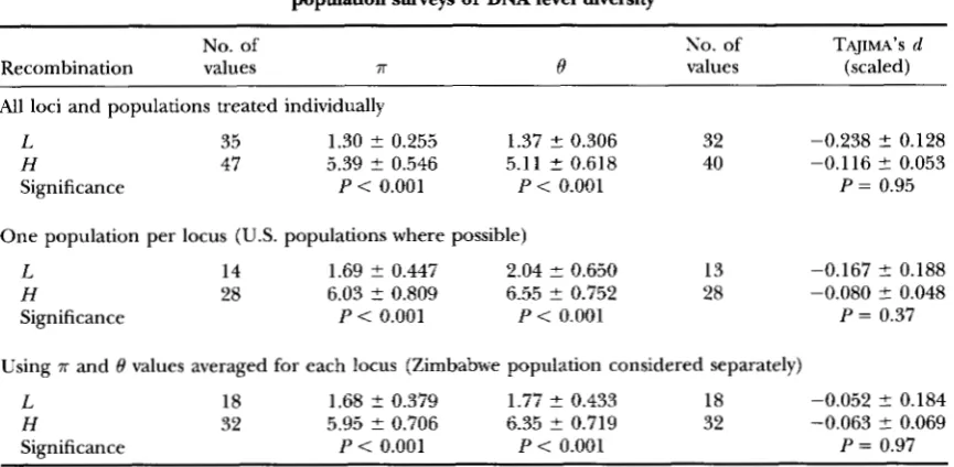
TABLE 6

Results of TAJIMA’S tests for 50 loci studied in Drosophila melanogaster

population surveys of DNA level diversity

1629

No. of

Recombination values T

No. of TAJIMA’S d

0 values (scaled)

All loci and populations treated individually

L 35 1.30 f 0.255 1.37 2 0.306 32 -0.238 2 0.128

H 47 5.39 rt 0.546 5.11 2 0.618 40 -0.116 2 0.053

Significance P < 0.001 P < 0.001 P = 0.95

One population per locus (U.S. populations where possible)

L 14 1.69 f 0.447 2.04 f 0.650 13 -0.167 2 0.188

H 28 6.03 2 0.809 6.55 f 0.752 28 -0.080 2 0.048

Significance P < 0.001 P < 0.001 P = 0.37

Using T and 8 values averaged for each locus (Zimbabwe population considered separately)

L 18 1.68 2 0.379 1.77 f 0.433 18 -0.052 2 0.184

H 32 5.95 rt 0.706 6.35 f 0.719 32 -0.063 2 0.069

Significance P < 0.001 P

<

0.001 P = 0.97

The table shows estimates of variability in terms of the two standard measures (T and 8), for regions of low

recombination ( L ) compared with other chromosomal regions ( H ) . All values are multiplied by 1@. Values of TAJIMA’S statistic are shown in terms of unstandardized d values (T -

e),

scaled as described in the text.

SEs of the statistics are also given, and the levels of significance of the differences between results from the L and H recombination regions were tested by MANN-WHITNEY U tests. Note that numbers are lower for the TAJIMA statistics than for the diversity measures, because for some loci no diversity was detected, so that the statistic could not be calculated. The initial data source was the compilation of KREITMAN and WAYNE (1994). For sequencing studies published since that compilation, this was supplemented by data for silent and noncoding (intron and flanking) sites where available (LEICHT et al. 1994; SIMMONS et al. 1994) or with unpublished data for silent sites in coding regions complied by E. N. MORIYAMA and J. R. POWELL. We also included the SSCP study of AGUADE et al. (1994) and additional unpublished data supplied by C. F. AQUADRO, J. HEY, H. HILTON, E. C . KINDAHI., J. PRITCHARD and S. W. SCHAEFFER.

destroys diversity, the number of alleles should recover faster than T , and this should produce negative values

of TAJIMA’S D, or of Fu and LI’S D. In contrast to our results for background selection, significant values of TAJIMA’S and FU and LI’S test statistics in samples of realistic size occurred in a high proportion (>60% of one-tailed tests) of simulations in which hitchhiking caused greatly reduced diversity values (BRAVERMAN et al. 1995; SIMONSEN et al. 1995). WATTERSON’S test performed about as well as the other tests.

BRAVERMAN et al. (1995) compared their simulation results with five studies of molecular variation in D.

melanogastm, where the loci surveyed were in regions of very low recombination and had substantially reduced levels of genetic diversity compared with typical values, and where there were enough segregating sites in the samples that tests of neutrality compared with the hitchhiking alternative had reasonable power. Only one of the cited studies in which TAJIMA’S D was calculated yielded a significant value, while diversity was reduced to -10% of the standard value for D. melanogaster.

Hitchhiking of the intensity required to explain this reduction in diversity would be very likely to produce significant Dvalues. These authors therefore concluded that severe hitchhiking alone cannot explain the low

genetic diversity observed. In contrast, our power analyses indicate that significant D values are unlikely to be detected if background selection had caused the low genetic diversity at these loci. In the published litera- ture to date (see Table 6 ) , three out of 51 values of TAJIMA’S standardized Dvalue significant at the 5% level have been found (two for the y-ac-sc region, and one for Adh-dup)

.

(12)

which may inflate estimates of variability, and produce discrepancies between x and d (see STROBECK 1987,

pp.

151-152). Taking the reported data at face value, it is, however, possible to compare T and d values, i.e., to calculate the unstandardized TAJIMA’S d, whose expectation is zero under neutrality. We did this for all studies that we could find, whether based on restriction enzyme or SSCP surveys of loci and their surrounding sequences, or on sequencing studies of individual loci. Where both restriction and sequencing studies were available for the same locus in a given population, we used the restriction enzyme data, as these generally had larger sample sizes and usually include noncoding sequences.

Out of 82 pairs of values, including 50 loci, we classi- fied 35 (18 loci) as coming from regions with low recombination (loci in X chromosomal bands 1-3A4, bands 21, 38-43E, and 59E-60 of chromosome 2, and bands 61-62A, 78-84 and 100 of chromosome 3), and 47 as representing regions with more recombination (see LANGLEY et al. 1988). Because selection events such as hitchhiking might occur within one population but not another, it is most appropriate to calculate TAJIMA’S d values for data from single populations. For measures of diversity, however, it may be preferable to calculate estimates from data combined from as many populations as possible. We therefore treated the data in several different ways (see Table 6).

Genetic variability was significantly reduced in the low recombination regions as defined above, for both

x

and 0 values, averaging 0.24-0.32 of the values estimated for the other loci, depending on how the data were treated (Table 6 ) . Because differences between x and 0, from which TAJIMA’S d values are calculated, will tend to be smaller when the diversity measures are themselves small, i.e., in the regions with low recombination, we scaled each value by dividing by the mean

d value for the loci in its set (data from either low recombination regions or from loci in the other regions) and compared the scaled d values. Unlike the diversity measures, there was no significant difference in d between the two recombinational environments, the values being slightly negative for both sets of loci with a slight tendency for the samples from loci in low recombination regions to have larger negative values (Table 6). The data thus suggest that there may be a slight overall excess of rare alleles, compared with the neutral expectation, due either to selection on the sites studied or on linked sites. The departure is, however, significant only in one of the six tests (for the H loci in the upper set of results in Table 6), and this result is rendered doubtful by the evident lack of independence between the different data sets for the same loci.

The data thus provide no clear evidence favoring hitchhiking but appear consistent with the reduction of variability in low recombination regions having been caused by background selection. The d values from

these studies were similar to values resulting from our simulations, when scaled in the same manner. For the samples of size 100, for instance, with the parameter values of Table 2 and either high or low mutation rates to deleterious alleles, the d value scaled in the same way was -0.066. These results cannot, however, be considered as strong evidence in favor of background selection as the sole cause of reduced genetic variation, relative to neutral expectation, as other possibilities that preserve the neutral pattern of alleles frequencies may also exist. GILLESPIE (1994) has, for instance, shown that a model of fluctuating selection, involving the ultimate fixation or loss of weakly selected alleles, can also lead to reduced genetic diversity without generating a large difference between the effect on x and 0, so that sig- nificantly negative D values would presumably not be found in samples. Thus, the observation of reduced variability without significant departures of allele frequencies from neutral expectation does not necessarily mean that background selection is the force involved.

In our previous study of the effects of background selection (CHARLESWORTH et al. 1993), we concluded that this process alone was not a plausible explanation for the great reduction in genetic diversity in some regions of the D. melanogastergenome, such as the tip of the X chromosome and the fourth chromosome. The reason was that it is unlikely that rates of deleterious mutation in such small regions of the genome would be high enough to make background selection a powerful force. This conclusion should now, however, be qualified. Good approximate methods for large populations have recently been developed that enable model- ing of the effects of background selection in the presence of- genetic recombination (R.

R.

HUDSON and

N. L. KAPLAN 1995; M. NORDBORG, B. CHARLESWORTH and D. CHARLESWORTH, unpublished results). These

methods can be used to predict levels of genetic diversity in different regions of the Drosophila genome, for which some of the relevant parameters can be estimated, and data on reduced variability in the centro- meric regions of chromosomes can be fitted reasonably well

(R.

R.

HUDSON and N. L. KAFTAN, unpublished results; B. CHARLESWORTH and

R.

R. HUDSON, unpublished results). The data on reduced variability at loci on the tip of the X and the fourth chromosome can also explained if the effects of transposable element insertions are taken into account (B. CHARLESWORTH

and

R. R.

HUDSON, unpublished results). As noted by

HUDSON (1994), transposable elements may play an important role in background selection, since the available evidence suggests that such elements are usually mildly deleterious in their effects on fitness and are distributed over many sites in the genome