Push-over analysis method - definition of conversion factors of the capacity curve depending on the load profile

(1)

Division V

PUSH-OVER ANALYSIS METHOD – DEFINITION OF CONVERSION

FACTORS OF THE CAPACITY CURVE DEPENDING ON THE LOAD

PROFILE

Jean-Marc Vezin1, Nader Mezher1, Véronique le Corvec1, Thibaud Thénint1

1

NECS, 196 rue Houdan, 92330 Sceaux, France ([email protected])

ABSTRACT

The push-over analysis method is now recognized by international standards as one of the reference method for seismic structural analysis. This paper deals with one step of the method: the conversion of the capacity curve of the structure to the behaviour diagram of the equivalent SDOF oscillator. The numerous publications about push-over method provide guidance on these factors, but do not give a rigorous definition. This paper reminds the theoretical foundations of the push-over analysis, from which one deduces the rigorous definition of the conversion factors, depending on the structure, the load profile, and the choice of the control point. An example illustrates the influence of these factors.

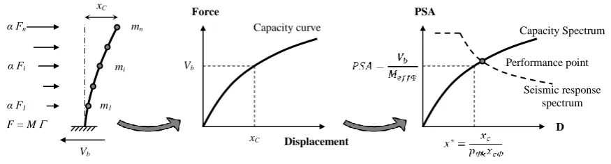
Figure 1. Principals of the push-over method

INTRODUCTION

The push-over analysis method is now recognized by international standards as one of the reference method for seismic structural analysis (ATC 40, FEMA 356 et 440, NF EN 1998). Furthermore, the term push-over covers not only one method, but many derivatives, based on the same principles.

The principles of this method are well known and detailed in numerous publications (Chopra & Goel, 1999 ; Krawinkler, 1996). It involves representing the structural seismic response by a progressive static loading, assessing the nonlinear response of the structure under this loading, and determining the performance point of the structure.

One of the main basis of this method is the assumption that the structure behaves as a nonlinear Single Degree of Freedom Oscillator (SDOF) whose behaviour is determined according to the nonlinear structural response under the static incremental loading. The SDOF behaviour curve is constructed in the ADRS (Acceleration - Displacement Response Spectrum) coordinates system by

m1

mi

mn

α F1

α Fi

α Fn

xC

Vb

Capacity curve

Force

Displacement Vb

xC

Capacity Spectrum

PSA

D

Seismic response spectrum Performance point

(2)

transformation of the Capacity Curve of the structure (Global Force - Displacement of Control Point) by conversion factors applied on the abscissa and ordinate.

The numerous publications about push-over provide guidance on these factors, but do not give a rigorous definition. In fact, the conversion factors depend on the structure behaviour, the choice of the Control Point, and the load profile.

This paper reminds the theoretical foundations of the push-over analysis, from which one deduces the rigorous definition of the conversion factors, depending on the structure, the load profile, and the choice of the control point (Note: this is not the aim of this paper to validate the relevance of the assumptions regarding the load profile or the control point, but only to give rigorous tools to calculate the conversion factors). An example illustrates the influence of these factors.

FORMULATION OF PUSH-OVER ANALYSIS FOR A GIVEN LOADING PROFILE

Formulation of the dynamic problem

In the context of a structural analysis by the Finite Element Method (FEM), the structure is represented by its stiffness matrix K, its mass matrix M and its damping matrix C. The dynamic equation of the structure’s relative displacement under the effect of an unidirectional ground motion is:

𝑀𝑈̈(𝑡) + 𝐶𝑈̇(𝑡) + 𝐾𝑈(𝑡) = −𝑀𝑘(𝑡), with (1)

U(t) = relative displacement vector

k = unit vector in the direction of excitation, k = x, y or z (i.e. a vector with all components equal to zero except the one corresponding to the k direction set to 1)

(t) = ground motion acceleration

The principle of push-over analysis is based on the assumption that the time history structural response U(t) is proportional to a reference deflection shape :

𝑈(𝑡) = 𝛼(𝑡) (2)

This reference deflection shape should represent the seismic response of the structure. It’s generally the main eigen mode if the structure has a mono-modal behaviour. Otherwise, the reference deflected shape is calculated under a static loading representative of the seismic action. We consider the general case of a reference loading defined by an acceleration field  in the structure:

𝐹 = 𝑀= 𝐾 (3)

Hence = 𝐾−1𝐹 = 𝐾−1𝑀 (4)

Substituting U(t) by (t) in (1), and multiplying it by t, the matrix equation (1) becomes a scalar equation, and the MDOF problem is converted into a SDOF problem:

𝑡_𝑀__{𝛼̈(𝑡) +}_𝑡_𝐶__{𝛼̇(𝑡) +}_𝑡_𝐾__{𝛼(𝑡) = −}_𝑡_𝑀_

𝑘(𝑡) (5)

or 𝑡_𝑀__{𝛼̈(𝑡) +}_𝑡_𝐶__{𝛼̇(𝑡) +}_𝑡_𝑀__{𝛼(𝑡) = −}_𝑡_𝑀_

𝑘(𝑡) (6)

We define the following parameters depending on the load profile and the associated reference deflection shape:

participation factor : 𝑝_𝑘 =

𝑡_𝑀_ 𝑘

𝑡_𝑀_ (7)

(3)

generalised damping : 𝐶∗=𝑡𝐶 (9)

generalised stiffness : 𝐾∗=𝑡𝐾=𝑡𝑀 (10)

We introduce a variable change:

𝛼(𝑡) = 𝑝_𝑘𝑥∗(𝑡) (11)

We obtain the equation of the equivalent SDOF oscillator:

𝑀∗_𝑥̈∗_{(𝑡) + 𝐶}∗_𝑥̇∗_{(𝑡) + 𝐾}∗_𝑥∗_{(𝑡) = −𝑀}∗__(𝑡) ₍₁₂₎

The pseudo-acceleration of the equivalent SDOF oscillator is then:

𝑃𝑆𝐴 =∗2_𝑥∗₌ 𝐾∗

𝑀∗𝑥∗ (13)

In spectral analysis, the maximum response of the oscillator is given by the response spectrum in relative displacement Sd(*; ) or in pseudo-acceleration Sa(*; ) = *² Sd(*; ):

𝑥𝑚𝑎𝑥∗ = 𝑆𝑑(∗;) = 𝑆𝑎(∗;)

∗2 =

𝑀∗ 𝐾∗𝑆𝑎(

∗_;_₎ ₍₁₄₎

Calculation of the Capacity Curve of the structure

The static response of the structure is computed using a nonlinear model of the structure, under an incremental progressive loading proportional to the reference load profile F. Thus, the displacement field of the structure U() is calculated for a loading  F,  varying from 0 to max.

The capacity curve of the structure is the diagram representing the relation between the total base shear force Vb and the displacement xc of a point of the structure named Control Point (see Figure 1). The Control Point is chosen to be representative of the global behaviour of the structure. Usually, the Control Point is chosen at the top of the building. However, it is interesting to consider several control points, in order to assess the results variability depending on the chosen control point.

Transformation of the Capacity Curve into Capacity Spectrum

The transformation of the Capacity Curve into Capacity Spectrum aims to define the nonlinear behaviour law of the SDOF oscillator equivalent to the structure. The Capacity Curve is defined in Acceleration-Displacement (A-D) coordinates. It allows determining the Performance Point of the structure under seismic load, by its intersection with the seismic Response Spectrum (itself also converted into A-D coordinates).

This transformation is defined by a double affinity applied on the abscissa and the ordinates of Capacity Curve.

On the abscissa, the conversion factor should transform the Control Point displacement into the SDOF equivalent oscillator displacement. Its formulation is derived from equations (2) and (11) which give a relation between the structure’s displacement field and the SDOF equivalent oscillator displacement, using the reference deflected shape :

𝑈 = 𝛼 = 𝑝𝑘𝑥∗ (15)

This equation is valid on each point of the structure. Writing it at Control Point, we obtain the following conversion formula:

𝑥∗₌ 𝑥𝑐

(4)

Thus, the displacement conversion factor is equal to the product of the participation factor pk calculated for the reference deflected shape  (see equation 7), by the control point displacement xc in the same deflected shape .

On the ordinate, the conversion factor should transform the base shear force into the pseudo-acceleration of the SDOF equivalent oscillator. This factor is a mass quantity, and is named Meff (effective mass associated to the reference deflected shape ):

𝑃𝑆𝐴 = 𝑉𝑏

𝑀𝑒𝑓𝑓 (17)

The base shear force is equal to the sum of forces applied to the structure in the seismic direction:

𝑉𝑏=𝑘𝑡𝛼 𝐹 =𝑡𝑘𝑀 𝑝𝑘𝑥∗ (18)

By combining equations (17) and (18) with (13), (8) and (10), we obtain the formulation of the effective mass:

𝑀𝑒𝑓𝑓 =

𝑡_𝑀_ 𝑘𝑘𝑡𝑀

𝑡_𝑀_ (19)

This effective mass is an extension of the standard concept of the effective mass used in modal-spectral analysis, generalised to any inertial load profile. The meaning of this effective mass can be checked for two specific cases of loadings:

- If the load profile follows the shape of an eigen mode of the structure i, then  = i and  = i² i. Therefore, 𝑀𝑒𝑓𝑓= (𝑡𝑖𝑀𝑘)²/(𝑖𝑡𝑀𝑖) which is exactly the eigen mode effective

mass.

- If the load profile is an uniform acceleration:  = k, then 𝑀𝑒𝑓𝑓 =𝑘𝑡𝑀𝑘 = 𝑚𝑡𝑜𝑡, which is

the total mass of the structure.

Influence of the nonlinear structural behaviour on the conversion factors

Generally, the conversion factors pk xc and Meff are determined with the assumption of linear elastic behaviour of the structure, which is realistic if seismic loading is low.

When the loading increases in the push-over analysis, the deflected shape could differ from the initial shape, more or less significantly. Some authors suggest taking into account the influence of this shape change by an adaptative loading, whose shape changes at each load increment according to the new deflected shape (FEMA 440). Other possibility consists of maintaining a constant load shape while updating the conversion factors at each loading increment according to the new deflected shape. The influence of load profile may also be analysed, considering several different load profiles.

Thus, the conversion factors may be updated at each load increment in the push-over analysis. Therefore, pk xc and Meff are recalculated at each load increment, replacing the reference deflected shape  by the actual deflected shape U(). Finally, with one given static nonlinear analysis under a given load profile, we can derive several capacity spectra:

- One capacity spectrum may be defined considering the constant conversion factors pk xc and

Meff. If several control points are considered, each of them will lead to a different capacity spectrum.

- An additional capacity spectrum may be defined considering the variable conversion factors: pU()k xc U() and Meff U(). With these assumptions, the capacity spectrum is defined by 𝑥∗=

𝑥𝑐 𝑈(𝛼)/(𝑝𝑈(𝛼)𝑘𝑥𝑐 𝑈(𝛼)) = 1/𝑝𝑈(𝛼)𝑘 and 𝐴 = 𝑉𝑏/𝑀𝑒𝑓𝑓𝑈(𝛼). It is noticeable that x* no longer

(5)

By comparing these different spectra one can notice the scatter in results based on different assumptions, and therefore this is an indicator of uncertainties. If all spectra are close, it means that the deflected shape of the structure remains relatively proportional to the reference deflected shape, and so the results are not significantly affected by the choice of control point. On the contrary, the results dispersion is a good indicator of uncertainties in the seismic structural behaviour, and it has to be taken into account in the results analysis.

EXAMPLE OF APPLICATION

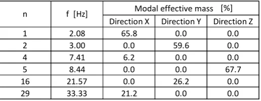
The studied structure is a simple regular reinforced concrete building with 3 levels, each 4 m heigh. The structure is made up of two portal frames ensuring floors bearing and bracing in longitudinal X direction, two walls ensuring bracing in transverse Y direction, 3 floors and a base slab. The structure and its finite element model are described in detail in (Thénint, 2015). The model is shown on figure 2 and its main eigen modes are presented in table 1.

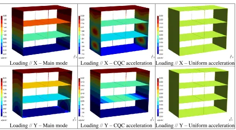
Several push-over analyses are carried out, for each earthquake direction (X and Y), considering successively 3 different loading profiles (see figure 3):

- loading according to main eigen mode shape,

- acceleration profile according to spectral response (CQC superposition of modal responses),

- uniform acceleration.

Three different control points are considered, one at the centre of each floor, in order to evaluate the results variability depending on the chosen control point.

Figure 2. General view of finite element model (mesh and volumic representation)

Table 1. Main eigen modes and associated effective masses

The table 2 presents, for each direction and loading profile, the constant conversion factors (CF), calculated according to the reference deflected shape based on a linear elastic analysis. It is noticeable that the effective mass significantly varies depending on the loading profile. In case of modal loading, we find the effective mass of the main mode (66 % of the total mass in X direction and

Direction X Direction Y Direction Z

1 2.08 65.8 0.0 0.0

2 3.00 0.0 59.6 0.0

4 7.41 6.2 0.0 0.0

5 8.44 0.0 0.0 67.7

16 21.57 0.0 26.2 0.0

29 33.33 21.2 0.0 0.0

Masse modale effective [%]

(6)

60 % in Y direction). In case of uniform acceleration loading, we find the total building mass (822 t). In case of CQC acceleration load profile, we find a value in between the two previous ones. This is consistent with the CQC load profile which is between the modal profile (which is quasi-triangular) and the uniform profile. Regarding the displacement CF, they are almost identical for the 3 load profiles. The difference is less than 1 % for the roof control point, and slightly increases (< 5 %) for the control points of lower floors.

The table 3 presents the variable CF, calculated according to the deflected shape of the nonlinear model under progressive loading. The CF are calculated at each loading increment, which allows assessing their range of variation. It is noticeable that for this regular structure, the CF vary very little while loading increases. The variation is less than 1 % for the roof control point. For the control points at lower floors, the CF variation is more significant, but it remains low (< 7 %). It can be concluded that for this regular building, the nonlinear deflected shape remains relatively proportional to the reference linear elastic deflected shape.

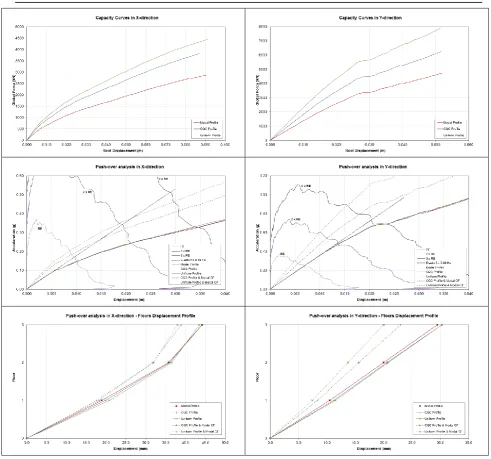
The figure 4 presents a summary of the main results of push-over analysis, for each direction and each loading profile. The chosen control point is located at roof level. The first series of graphs present the capacity curves for the three loading profiles. The second series presents the capacity spectra derived using the CF specific to each loading profile. By way of comparison, we present also (dashed lines) the capacity spectra calculated by applying the same CF for all load profiles, based on the effective mass and the participation factor or main eigen mode. This approach corresponds to the usual practice, in the absence of a rigorous definition of conversion factors. The capacity spectra are superimposed to a seismic demand spectrum (reference earthquake RE), and its multiples (2 x RE and 3 x RE). The third series of graphs presents the floors displacement profile for the performance point at earthquake level 3 x RE.

The comparison of results shows the importance of using the appropriate conversion factors corresponding to each loading profile:

- With the appropriate conversion factors, the 3 loading profiles lead to almost identical capacity spectra, and the floor displacement are very close.

- When the conversion factors are arbitrarily fixed based on the main eigen mode, the CQC and uniform loading profiles lead to inaccurate results which significantly differ from those of modal profile. The capacity spectrum is over-estimated, and its initial slope does not match to the eigen frequency of the structure (slope = ² = (2f)²). The floor displacements are under-estimated by 10 % in X direction, and 35 % in Y direction.

(7)

Loading // X – Main mode Loading // X – CQC acceleration Loading // X – Uniform acceleration

Loading // Y – Main mode Loading // Y – CQC acceleration Loading // Y – Uniform acceleration

Figure 3. Studied acceleration distribution

Table 2. Constant conversion factors based on the linear elastic reference deflected shape

Table 3. Variable conversion factors based on the deflected shape of the nonlinear model under progressive loading (minimum and maximum values over all loading increments)

modal CQC uniform modal CQC uniform

541 731 822 490 655 822

roof 1.27 1.27 1.26 1.29 1.30 1.30

2nd floor 1.01 1.01 1.02 0.87 0.88 0.89

1st floor 0.57 0.59 0.60 0.45 0.46 0.47

Factor

Meff (t)

Loading profile // X

pk xc

Loading profile // Y

modal CQC uniform modal CQC uniform

538-542 730-732 822 491-492 654-656 822 roof 1.26-1.27 1.25-1.27 1.24-1.25 1.29-1.30 1.30 1.30 2nd floor 1.01-1.02 1.01-1.03 1.02-1.04 0.87-0.89 0.88-0.89 0.89-0.90

1st floor 0.53-0.57 0.56-0.59 0.59-0.61 0.47-0.45 0.47-0.48 0.48-0.50 Meff (t)

pk xc

(8)

Figure 4. Results summary of push-over analysis

(9)

CONCLUSION

The push-over analysis is based on the assumption that the structure behaves as a nonlinear single degree of freedom oscillator. One important stage of the method is the transformation of the capacity curve of the structure (Global Force - Displacement of Control Point) into capacity spectrum of the equivalent SDOF oscillator (Acceleration - Displacement).

This paper provides a rigorous formulation of the conversion factors, depending on the structure, the load profile, and the choice of the control point.

An application carried out for an example of regular building shows the importance in using the appropriate conversion factors. The use of identical conversion factors regardless the loading profile may lead to inaccurate and unsafe results. Thus, in the studied example, when we consider the loading profiles different of modal shape (CQC or uniform profile), while using the conversion factors calculated according to modal shape, the floor displacements are under-estimated by 10 to 35 %.

The application to other structures would allow drawing more general conclusions, especially regarding the results variability depending on the choice of the control point, and the relevancy of using constant or variable conversion factors depending on the loading level.

REFERENCES

ATC 40, “Seismic evaluation and retrofit of concrete buildings”, vol. 1, Applied Technology Council, November 1996.

A.K. Chopra, R.K. Goel, "Capacity-demand-diagram methods for estimating seismic deformation of inelastic structures: SDF systems”, Report No. PEER-1999/02, University of California, Berkeley, April 1999.

Clough & Penzien, Dynamics of Structures, Third Edition, Computers & Structures Inc., 1995.

FEMA 356, “Prestandard and commentary for the seismic rehabilitation of buildings”, November 2000.

FEMA 440, “Improvement of nonlinear static seismic analysis procedures”, June 2005.

Krawinkler H., “Push-over analysis: ‘Why, how, when and when not to use it’”, 65th annual convention of SEAOC, October 1-6, 1996.

NF EN 1998-1 et NF EN 1998-3, EC8, Calcul des structures pour leur résistance au séisme, 2005.