INTEGRATED IMPERFECT PRODUCTION PROCESS WITH EXPONENTIAL DEMAND RATE

-175-

Aryabhatta Journal of Mathematics & Informatics Vol. 6, No. 1, Jan-July, 2014 ISSN : 0975-7139 Journal Impact Factor (2013) : 0.489

INTEGRATED IMPERFECT PRODUCTION PROCESS WITH

EXPONENTIAL DEMAND RATE

Naresh Kumar Kaliraman*, Ritu Raj**, Dr Shalini Chandra*** and Dr Harish Chaudhary****

*Research Scholar, Centre for Mathematical Sciences, Banasthali University, P.O. Banasthali Vidyapith, Banasthali – 304022, Rajasthan, India • e-mail:dr.nareshkumar123@gmail.com

**Research Scholar, Centre for Mathematical Sciences, Banasthali University, P.O. Banasthali Vidyapith, Banasthali – 304022, Rajasthan, India • e-mail: rrituiit@gmail.com

*** Associate Professor, Centre for Mathematical Sciences, Banasthali University, P.O. Banasthali Vidyapith, Banasthali – 304022, Rajasthan, India • e-mail: chandrshalini@gmail.com

****Assistant Professor, Department of Management Studies, Indian Institute of Technology, Delhi, New Delhi-110016, India • e-mail: hciitd@gmail.com

ABSTRACT:

This paper is developed a three layer supply chain production-inventory model for supplier, producer and retailer. The model speculates exponential demand and production rate for all member of three-layer supply chain. The model deliberates the effect of commercial policies such as exponential demand rate; production rate is demand dependent, perfect order size of raw material, unit manufacturing price and idle times in assorted sectors on integrating marketing framework. The basic assumption of the model is that manufacturing items are of perfect and imperfect quality. This technique used in different types of production industries like electrical and electronics, paper, pharmaceutical, automobiles etc. Mathematical modeling is used to derive the production rate and order size of raw material for maximum total profit of supply chain. A numerical example including the sensitivity analysis is validated to the outcomes of the production-inventory model.

Keywords: Exponential Demand Rate, Imperfect Production Process, Integrated, Supply Chain

1. INTRODUCTION:

Naresh Kumar Kaliraman, Ritu Raj, Dr Shalini Chandra and Dr Harish Chaudhary

despatching position. Wee et al. [2007] and Eroglu and Ozemir [2007] accumulated the model of Salameh and Jaber [2000], letting shortages. In a realistic manufacturing surroundings, the defective quality objects could be revised and reconstructed (Sana and Choudhary [2010]; Sana [2010, 2010a]; Sarkar et al. [2010]); therefore, generally manufacturing inventory charges can be condensed prominently (Hayek and Salameh [2001]; Chiu [2003]; Chiu et al. [2004, 2006]). Whole phases from delivery of raw materials to finished goods can be incorporated in a supply chain, consolidating supplier, manufacturer, retailer and customers. A three layer supply chain depends on better performance of business strategies like price, better delivery of goods, quantity deduction, quantity up and down, guarantee of purchase quantity etc. Goyal and Gunasekaran [1995] extended an integrated model for defining the economic production quantity and economic order quantity for raw materials in multi-stage manufacturing framework. Aderohunmu et al. [1995] accomplished the savings of both the retailer and customer when they monitored a supportive approach and mutual cost message along with other information in time. Thomas and Grifin [1996] studied that effective supply chain system needs arrangement and management between the system followers including producers, vendors and mediators if any. Narsimhan and Carter [1998] expressed, a good supply chain system totally depends on the combination of supply of goods and management between providers, producers and consumers. Munson and Rosenblatt [2001] developed two level supply chains to a three level supply chain, including a provider, a producer and a vendor where producer was leader of the supply chain system. Yang and Wee [2001] developed a three-layer supply chain model including supplier, manufacturer and retailer. They proved that cost reduction is more important instead of individual decision of each member of supply chain. Khouja [2003] presumed three-layer system between the followers of the supply chain that lead to significant contraction in total cost. Cardenas-Barron [2007] accumulated the model of Khouja [2003] by numerical technique, including n-stage multi-customer supply chain inventory system. Yao et al. [2007] developed an analytical model that allocate the important supply chain limits, specifically ordering costs and carrying charges, affects the inventory cost savings.

The projected model deliberates a three-layer supply chain including supplier, producer and retailer, who are reliable for execution of the raw materials into finished goods and mark them obtainable to gratify consumer’s demands in time. Inventory and manufacturing policies are prepared at the supplier, producer and retailer stages. The challenge is to accomplish inventory and manufacturing policies through the supply chain so that the total anticipated profit of the supply chain is maximized.

The remnant of this paper is arranged as follows: Section 2 describes essential assumptions and notations. Section 3 describes mathematical model and solutions. Section 4 describes numerical example. Section 5 describes sensitivity analysis. Section 6 concludes the paper. A list of references is also provided.

2. ESSENTIAL ASSUMPTIONS AND NOTATIONS

The mathematical model is developed on the bases of following assumptions:

1. The demand rate is exponential increasing function of time. 2. Production rate is demand dependent

i.e.

P t

 





D t

 

, where

D t

 



be

at

and





1

3. Production cost per unit is a function of production rate. 4. Idle time costs are assumed at supplier’s and producer’s level.

Integrated Imperfect Production Process With Exponential Demand Rate

6. Single item products are considered for joint effect of supplier, producer and retailer in a three layer supply chain.

7. Replenishment rate is instantly infinite but its size is finite at producer’s level. 8. Insignificant lead time.

The mathematical model is developed on the bases of following notations: Q Supplier’s replenishment lot size.

at

be



Producer’s production rate that is equal to supplier’s demand rate.



Supplier’s proportional probability of imperfect items with probability density function

f

 



.

A

S

Supplier’s set up cost.

r

s

Supplier’s screening rate per unit time.

s

S

Supplier’s screening cost per unit item.

h

s

Supplier’s holding cost per unit time.

I

S

Supplier’s cost per unit idle time.

s

C

Supplier’s purchasing cost per unit item.

w

s

Supplier’s selling price per unit perfect items.

w

s

Supplier’s selling price per unit imperfect items.

 

E x

Expectation of variable

x

.

SAP

Supplier’s average profit.

ESAP

Supplier’s expected average profit.



Producer’s proportional probability of imperfect items with probability density function

g

 



.

p

A Producer’s set up cost.

p

r Producer’s screening rate per unit time.

p

S Producer’s screening cost per unit item.

p

h Producer’s holding cost per unit time.

I

p

Producer’s cost per unit idle time.

 

P C

Per unit item production cost.

p

w Producer’s selling price per unit perfect item.

p

w Producer’s selling price per unit imperfect item. PAP Producer’s average profit.

EPAP Producer’s expected average profit.

at c

be Customer’s demand rate.

at r

be Retailer’s demand rate.

A

r

Retailer’s set up cost.

h

Naresh Kumar Kaliraman, Ritu Raj, Dr Shalini Chandra and Dr Harish Chaudhary

w

r

Retailer’s selling price per unit item.

RAP

Retailer’s average profit.

ERAP Retailer’s expected average profit. T Retailer’s cycle length.

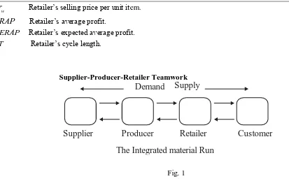
Supplier-Producer-Retailer Teamwork

Demand

Supply

Supplier

Producer

Retailer

Customer

The Integrated material Run

Fig. 1 3. MATHEMATICAL MODEL

In this projected model, supplier deliveries the raw materials at rate



beat to the producer up to manufacturing run time

t

₁. The imperfect objects at supplier are sent back after finished the assessment at one lot with sales rate

s

_w

per unit item to the external supplier where the raw materials are bought. The producer meets the demand of retailer at a rate be_ratupto time

kT k





1



. Throughout manufacturing run time

 

0,

t

₁ , inventory of best items stacks up with rate_



1

 



beatbe_rat_.The collected inventory_



1

 



beat be_rat_t₁ gratifies the demand of retailer through



t kT

₁

,



. The imperfect items



be

at are collected at time

t

₁ those are sold at lesser rate in one lot. Thus, inventory cost for imperfect items up to time

t

₁ is measured. The demand of customers is met with rate

at c

be by retailer where the supply rate of produced objects is sustained up to time

kT

. The collected inventory at time

kT

is



be_ratbe_cat



kT that gratifies the demand for the period



kT T

,



(See Fig. 1.). The leading differential equations at supplier, producer and retailer level are as follows:

3.1. Specific average profit of supplier

 

S

I

t

is an inventory of perfect objects. In this case, the lot size Qis detached with rate

r

_sat cost

S

_sper unit item, after compilation of detaching, the total imperfect items are sent back to the retailers where supplier bought at a price

s

_w per unit item. The leading differential equation is

 

'

1

, 0

at s

I

t

 



be

 

t

t

… (1) With

I

_S

  

0

 

1





Q

and

I

_S

 

t

₁



0

.

From equation

 

1

, we have

 



1





1



, 0 1

at s

b

I t e Q t t

a



_

Integrated Imperfect Production Process With Exponential Demand Rate

Now,

I

_S

 

t

₁



0

, we have

t

₁

1

log 1

a



1



Q

a

b













_



_





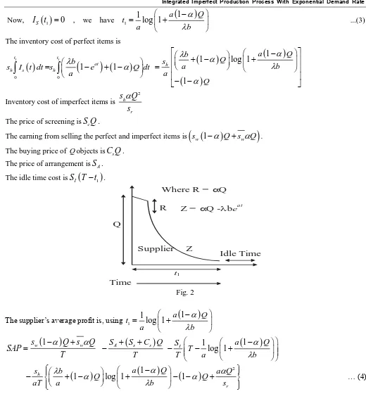
...(3)

The inventory cost of perfect items is

 









1 1

0 0

1

1

t t

at

h s h

b

s

I t dt s

e

Q dt

a



_







_



 

_





















1

1

log 1

1

h

a

Q

b

Q

s

a

b

a

Q





_







_

_









 

















_





_

_



_{ }







Inventory cost of imperfect items is

2

h

r

s

Q

s



The price of screening is

S Q

_c .

The earning from selling the perfect and imperfect items is



s

_w



1







Q



s

_w



Q



. The buying price of Qobjects is

C Q

_s .

The price of arrangement is

S

A.

The idle time cost is

S T

_I





t

₁



.

Q

Z Supplier

Idle Time R

Where R = Q

t1

Z = Q -bea t

Time

Fig. 2

The supplier’s average profit is, using

t

₁

1

log 1

a



1



Q

a

b













_



_





SAP



s

w



1



Q

s

w

Q

T









SA



Ss C Qs



T

 

 SI _T 1log 1 a



1



Q

T a b





   

 _    _

 

 













2

1

1 log 1 1

h

r

a Q

s b a Q

Q Q

aT a b s





_

_





    

  

 _   _{ }  _   _

 

   

  … (4)

3.2. Specific average profit of producer

 

p

I

t

is on-hand inventory of perfect items. In this stage, producer produces



beat objects per unit time where raw material is delivered with



beat rate up to the manufacturing run time

t

₁. Then, the differential equations are

  



'

1

1

at at

, 0

p r

I

t

 

 

be



be

 

t

t

... (5)

Naresh Kumar Kaliraman, Ritu Raj, Dr Shalini Chandra and Dr Harish Chaudhary

and

I

_p'

 

t

 

be

_rat

,

t

₁

 

t

kT

… (6)

with

I

_p

 

kT



0

From equations (5) and (6), we get

 













1

1

1 at 1 at , 0

p r

b b

I t e e t t

a a

 

  

      

  … (7)

and

 



₁ at





1





₁ at1



p r

b b

I t e e

a a

 



   

,

t

₁

 

t

kT

… (8)

Now,

I

_p

 

kT



0

, we have





1

1 1

log 1 1

akT r

e t

a





 _ 

 

 _  _



 

 







1

log 1 a 1 1

T Q

ak b





 

  _    _

  … (9)

The cost of arrangement isA_p

The earning from selling the perfect and imperfect items is

The cost of screening is 1 1





₁



₁



1

at akT

p p r

S



be S b





e



   

 The inventory cost of perfect items is

 

 











 

 



1

1 1

2

0 ₁

1 1

1 1 1

akT

t kT

r p

p p p p _at

t

akT e bh

HG h I t dt I t dt

a _{akT e akT at}

 

 

 

     

 

   

      

 







  

IO

Z

Producer _{Idle Time}

R

Where R = (1- ) b   eat

kT

Z = –be_rat

Time

IO = On-hand Inventory

Fig. 3

The inventory cost of imperfect items is







₁ 1 1







₁



₁



1

at at akT

p p p p r

w

 

be w



be w w



b





e



 

  _  _   



Integrated Imperfect Production Process With Exponential Demand Rate





1 2 2 2 1

1 0 t at at p p p b e

HD h be t t dt

r





         

















2 2 2 1 1 log 1 1 1 1 1 1 akT akT r r p akT r p e e h b

a _{a b e}

r

















 _  _      _ _       _{ }   _{ }      _{  }     

The total cost of manufacturing is

 

 





1 ₁ 1

1

akT

at er

P C



be P C



b





 _     _  _     

The unit manufacturing cost of finished product is

 

at

w p at

L

P C s be

be







   

Where

w

_s, the supplier’s buying cost per unit raw material, which is static,

p



is the static cost of finished product per unit.

at

L be



is equally distributed labor and energy cost over production size





at

be



.

at

be



is per unit instrument cost of finished product which is proportional to the magnitude of manufacturing rate



at



be



.

The producer’s average profit is



















1

1



1

1

₁

1

akT

akT _{p p r}

p r p

w

w

b

e

S b

e

A

PAP

T

T

T



_

_





_





_



_

_{ }







 

_

_

_

 





























2

1 1 1 1 1

1

1 log 1

1 akT akT r r p akT r

akT e akT e

bh

e

a T _akT













                           _{   }       













 









2 2 2

1

1

1

log 1

1

1

1

1

1

1

1

1

log 1

1

1

akT akT akT

p r r r

p

akT akT

r I r

h

b

_e

_e

_a

_b

_e

a T

r

P C

b

e

p

e

T

T

T

a



_

























_

_

_

_

_

_

_













_





_



_



_





_



_

_



























_





_







_



_







_





_





_



_

















… (10)

3.3. Specific average profit of retailer

 

r

I t

is on-hand inventory where producer deliver at ratebe_ratto the retailer up to time

kT

. After receiving customers demand at ratebe_cat, inventory stacks up with rate be_rat be_cat b e



_rate_cat



up to time

kT

. The collected inventory at time

kT

reduces and reaches to zero level at time

T

. Then, the leading differential equations are

 





'

, 0

at at

r r c

I t b e e  t kT … (11)

with

I

_r

 

0



0

Naresh Kumar Kaliraman, Ritu Raj, Dr Shalini Chandra and Dr Harish Chaudhary

with

I T

_r

 



0

From equations (11) and (12), we have r

 



rat cat



, 0

b

I t e e t kT

a

    … (13)

and r

 



rakT cat



,

b

I t e e kT t T

a

    …(14)

Now,

 

0

1

at c

r at

r

be

I T

k

be

  



as e_rat e_cat

For possibility of the model,

t

₁



kT



T

must be gratified. As stated,

kT



T

grasps as

k



1

. Now,

t

₁



kT

, we have ₁



1



1,



1



,

at

at at r at

r

be t

t e e

be

 

 



   



1



at _rat

E

e

e











… (15)

The cost of arrangement is

r

_A

The earning from selling items isr be T_{w c}at .

IO _{Retailer Z}

T

where Z = –be_ca t

Time

IO = On-hand Inventory

Fig. 4 The cost of buying objects is

w be T

_{p c}at .

The cost of inventory is

 

 

0

kT T

r h r r

kT

H r _ I t dt I t dt_







 2





1





akT aT

h r c

b

r e aT akT e

a

   

The retailer’s average profit is









2 1

at A at h akT aT

w c p c r c

r b r

RAP r be w be e aT akT e

T a T

       … (16)

3.4. Leader-Follower Association

In this case, producer is the leader; supplier and retailer are the followers. The producer bids followers to (i) buyback of the imperfect items, (ii) limited replacement charges with one time ordering cost (iii) assign buying costs, (iv) count the idle times of followers of the chain and (v) regular delivery agreement at every phase.

From equation (10), using 1





1

1

log 1

a

Q

t

a

b













_



_





,

akt at

r c

be be and T 1 log 1 a



1



1



Q

ak b





 

 _    _

Integrated Imperfect Production Process With Exponential Demand Rate

E [PAP] =





 

 

 



 



1

log 1 1 1

p

p p p p

p

h E b

ak b w E w E S P C akA

r

a

E E Q

b

 











               _{  }     







 



 







 



2 2

2

1

1

log 1

1

1

p p p

p p p

p

h

h

h

b

ak

w

E

S

P C

w

E

aE

Q

a

a

r

a

E

E

Q

b















_

_









_

_

_

_

_

_

_



_











_

_























_

_

_











  









 





 



2 2 2 2

1

1

1

log 1

1

1

p _{p p}

I

p

akh a E

E

Q

_bh

_h

_p

ak

E

E

Q

a

a

a

ak

r

E

E

Q

b















_

_





_









_



_

_

_



_

_















 



 







 



2 2

1

1

1

1

log 1

log 1

1

1

p p p I

bh

h

h E

b

p

aE

Q

ak

E

E

E

Q

a

a

a

a

b

a

E

E

Q

b

 





























































_

_

_











2

[ ] [ ( ) log(1 )

log(1 )

( ) log(1 )]

A

E PAP D FGQ HQ J LQ S BQ

BQ

K LQ M N PQ

      



    

…(17)

where

A



ak

, B aE



1

 

E 1



b





   , M h Ep

 

₂ b

a

 

 , N pI

a

 , P aE



1



b







 ,

G



aE



1







,



1



 

 

p

 

p p p p

p

h E

b

D

b w E

w E

S

P C

A

r

 

























_













_





















 



 



2 2

2

1

p p p

p p p

p

h

h

h

b

F

w

E

w

E

S

P C

a

a

r







































_







_























, I p S ak 

  







2 2 1 p p

h a E E H

r







 ,



1

 

1



p

h

L E E

a





   ,K bh₂p E



1



a





  ,J bh₂p

a



From equation (4), using

t

₁

1

log 1

a



1



Q

a

b













_



_





, akt at r c

be be and T 1 log 1 a



1



1



Q

ak b





 

 _    _

 

The supplier’s expected average profit is

E [SAP] =





 

 



 



2

1

log 1

1

1

h

w w s s A

r

I

aE

Q

s

akQ E

s

E

s

S

C

ak S

a

s

S

a

E

E

Q

Naresh Kumar Kaliraman, Ritu Raj, Dr Shalini Chandra and Dr Harish Chaudhary











 



1

1

log 1

log 1

1

1

h h I

aE

Q

b

k

s

E

Qs

S

a

b

a

E

E

Q

b





_















_

_

_



_













_

_





_

_

_











… (18)

From equation (16), using

t

₁

1

log 1

a



1



Q

a

b













_



_





, akt at r c

be be and T 1 log 1 a



1



1



Q

ak b





 

 _    _

 

The retailer’s average profit is



































 





2 1 1

1 1 1 1

log 1 1 1

1 1 1 1

log 1

akT A akT h akT akT

w r p r r r

akT

h A

w p r

h A

w p

h h

w p w p

A

r b r

RAP r be w be e aT akT e

T a T

r r

b r w k e

a T

r a akr

b r w k Q

a

a b

Q b

r r

b r w k a r w k Q

a a akr a













          _    _        _    _    _       _{    }        _    _ _    _       





1



1



Q

b





 _{ } 

 

 

The retailer’s expected average profit is

E [RAP] = h



1



h



1

 

1

 

1



w p w p

r r

b r w k a r w k E E Q

a a





 _{  } _  _{  }  _{ }

   

   



 



log 1 1 1

A

akr a

E E Q

b





  _{  }      … (19) Solution:

For optimum value of EAPP [Q], we have

log(1 )

EPAP A

Q BQ

 _

 

2

log(1

) (

) log

log(1

) (

) log

FG

HQ

L

BQ

K

M

N

LQ

P

L

PQ

J

LQ

S

B











 







_

_

_

_

_













 





 



2 2

log 1

log 1

log(1

)

D

FGQ

HQ

K

M

N

LQ

PQ

AB

J

LQ

S

BQ

BQ











 























_



_

We consider EPAP 0

Q 



 , which give us the value of Q













2 2

2

(

log

log )

(

log

log )

log

log

(

log

log

log

log

log

log )

H

L

B

L

P

BH

L

B

BL

P

H

L

B

L

P

BD

FG

K

B

M

B

N

B

K

P

M

P

N

P

Q

 



 









 

















Integrated Imperfect Production Process With Exponential Demand Rate

Again, we have the value of







 

2



2

3 2

2 2

log(1 ) log log

log(1 )

2 log(1 ) log(1 )

2

( ) log ( ) log

log(1 )

( ) log(1 )

( ) log(1 )

BQ H L B L P

B BQ

FG HQ L BQ L PQ

EPAP A

Q BQ K M N LQ P J LQ S B

D FGQ HQ K M N LQ PQ

B

J LQ S BQ

 _{  }         _{    }   _  _  _       _        _              _{ }  _{   }      Thus 2 2

0

EPAP

Q



_



grasps atQ satisfying inequality (15), then EPAP

 

Q

is maximum.

3.5. Integrated expected average profit

The integrated expected average profit of the supply chain is

EIAP=















 







 

 

 



 







 

 





1 1 2 2

1 1 1 1

1

log 1 1 1

2

1 1

p h

w p I I w p p h

p

p p p p A

p

p p p

p p p

p

kbh br

br bw p S k ar aw kh r k E E Q

a a

h E b

ak b w E w E S P C akA akr

r

a

E E Q

b

h h h b

ak w E S P C w E aE

a a r





 



















                                    _{  }            _{      }  _     _{ }          





 



 



  







 



 



1 1 2 2 2 2 1 1 1

log 1 1 1

1

log 1 1 1

h

A w w s s

p

r

p

Q s

akS ak E s E s S C

a

a

E E Q

b

a kE

akh a E E Q

s

a

r E E Q

b



















        _{ }  _  _ _{  }       _{ }        _{  }         _{ }          _{  }     





 



















 



1 1 1 1

1 1 1 log 1

log 1 1 1

p p

I I h p h

bh h E b aE Q

b

k p S s E h E s E Q

a a a b

a

E E Q

b     _{   }                             _{  }      EIAP=









 





2

1 1 1 1 1 1 1 1 1 1

1 1 1 1

1 1 1 1 1 1

log 1

log 1 log 1

H J Q K Q

D F Q G Q A B C Q

E C Q E C Q

 

 

  

Naresh Kumar Kaliraman, Ritu Raj, Dr Shalini Chandra and Dr Harish Chaudhary

where ₁ p h



1



w p I I

kbh

br

A

br

bw

p

S

k

a

a







_













_





B1



arwawpkhp rh



1k





,



 



1

1

1

C



E





E





, 1



1



 

 

 

p

p p p p A

p

h E b

D ak b w E w E S P C akA akr

r

 









  _      _    , 1 a E b  ,





 

 









 

2 2 1 2 1 1 1

p p p

p p p

p

h

A w w s s

h h h b

ak w E S P C w E aE

a a r

F

s

akS ak E s E s S C

a













              _   _              _{ }  _  _ _{  }     _ _      

  





2



2

 

2 1 1 1 p p r a kE

G akh a E E

r s







     _   _    ,





 

1 1 p p

I I h

bh h E b

b

H k p S s E

a a a

 



_

_

   _      _  ,













1 p 1 h 1

J k h E 



s E 



,





1 1 aE K b





 











 

 



2

1 1 1 1 1 1 1 1 1 1 1 1 1 1 1 1 1 1 1 1

log 1

1

log 1

log 1

D

F Q

G Q

H

J Q

K Q

A

B C Q

EIAP

E C Q

E C Q



























_

_



_

_

Solution:

Differentiating EIAP partially with respect to

Q

₁, we have













































1 1 1 1 1 1 1 1 1 1 1 1 1 1 1 1 1 1

1 1 1

1 1 1 1

2

1 1 1 1 1 1 1 1 1 1 1 1 1 1 1 1 1 1 1 2

1 1 1

2

log

log 1

log

log 1

log 1

log

1

log

1

log 1

F

G Q

C E

A

B C Q

B C

E C Q

K

H

J Q

J

K Q

EIAP

Q

E C Q

E C D

F Q

G Q

A

B C Q

E C Q

H

J Q

K Q

E C Q





















_

























For optimum value of

EIAP Q

 

₁ , put

1 0 EIAP Q    ,













































1 1 1 1 1 1 1 1 1 1 1 1 1 1 1 1 1 1

1 1 1

1 1 1 2

1 1 1 1 1 1 1 1 1 1 1 1 1 1 1 1 1 1 1 2

1 1 1

2 log log 1 log

log 1

log 1 ₀

log 1 log 1

log 1

F G Q C E A B C Q B C E C Q K H J Q

J K Q

E C Q

E C D F Q G Q A B C Q E C Q H J Q K Q

E C Q

Integrated Imperfect Production Process With Exponential Demand Rate

























2 2

1 1 1 1 1 1

1 1 1 1 1 1 1 1 1 1 2

1 1 1 1 1 1

1 1

2 3

1 1 1 1 1 1 1 1 1 1

1 ₂

3

1 1 1 1 1 1 1 1 1 1

2 2 log 2 log

log log logJ

2 log log 4

log

log log

2 log log

G B C E J K

C D E F B C C H E

G B C E J K

H K

C G E B C E C J E K

Q

C G E B C E C J E K

            _{   }       

   … (22)

Again, we have













































2

1 1 1 1 1 1

1 1 1

1 1 1 1 1 1 1 1 1 1 1 1 1 1 1 1

2

1 1 1 1 1 1 1

2 2

1 _{1 1 1}

2 2 2

1 1 1 1 1 1 1 1 1 1 1 1 1 1 1 1 1 1 1

log log

log 1

2 log log 1

log log 1

2

log 1

log 1 log 1

log 1

G B C E J K

E C Q

F G Q E C A B C Q B C E C Q

E C

K H J Q J K Q

EIAP

Q _{E C Q}

E C D F Q G Q A B C Q E C Q H J Q K Q

E             _{   }   _{ }     _          









3

1C Q1 1

                            Thus, 2 2 1

0

EIAP

Q



_



hold at

Q

1, and then

EIAP Q

 

1 is maximum.

4. NUMERICAL EXAMPLE: Example 1:

The following parameters in applicable units are considered as:

$400

A

S



,

s

_r



185, 000

units per unit time,

C

_s



$20

per unit,

S

_s



$0.6

per unit,

b



2

per unit,

k



0.5

per unit,

$3.5

h

s



per unit per unit time,

S

_I



$30

per unit time,

a



0.7

per unit,

s

_w



$70

per unit,

s

_w



$40

per unit,

$5000

p

A  ,r_p 180, 000units per unit time, S_p $0.8per unit, h_p $4.5per unit per unit time,

p

_I



$20

per unit time, wp $600per unit, wp $400per unit, 300

at c

be  units,

r

_A



$4000

,

r

_h



$6

per unit per unit time,

$620

w

r



per unit,



_p $2.5per unit,



$0.02per unit,





$1.5

per unit,

L



$4500

,

 

1 , 0.3 0.04

f







0.04

 



0.3

,

 

1

0.3 0.05

g





 , 0.05 



0.3.

The ideal outcome for integrated framework is Q21.90 units,

ERAP



$2960

,

ESAP



$164.40

,

$1006.80

EPAP



. Total profit of the supply chain is

$4131.20

.

 



   







0.3 0.3 2 2 2 0.04 0.04

0.04

0.3

1

1

1

0.3

0.04

0.3 0.04

0.26

2

2 0.26

1

0.0884

0.09 0.0016

0.17

Naresh Kumar Kaliraman, Ritu Raj, Dr Shalini Chandra and Dr Harish Chaudhary

Example 2:

The following parameters in applicable units are considered as: The values of the parameters in Example 1 are identical except

.

The ideal outcome for integrated framework is Q22.04 units,

ERAP



$2960

,

ESAP



$179.80

,

$1017

EPAP



. Total profit of the supply chain is

$4156.80

.

From Example1 and Example2, expected average profit of the supply chain with exponential demand is maximum.

5. SENSITIVITY ANALYSIS:

To know, how the optimal solution is affected by the parameters, we derive the sensitivity analysis for all

parameters. From the given numerical example, we derive the finest solution for a static subset. The finest values of all parameters in the subset increases or decreases by5%, 5% and10%, 10% . The results of total profit are existing in the following table 1.

TABLE 1

0 0

I I

Integrated Imperfect Production Process With Exponential Demand Rate

6. CONCLUSION:

Naresh Kumar Kaliraman, Ritu Raj, Dr Shalini Chandra and Dr Harish Chaudhary

at low price. A uniform distribution function is followed by the proportional influence of imperfect items. The cost of a unit of manufacturing is a function of manufacturing budget. We consider that producer as leader of the chain and the supplier and retailer are the followers of that chain. The total profit of producer is maximized. The integrated profit is also maximized by adding the profit of supplier, producer and retailer. Chief contributions of this research are exponential demand rate, production rate is demand dependent, idle times, finite replenishment rate and effect of imperfect items on the three-layer supply chain. The unit production cost is increases because the servicing costs of remedial and preclude maintenance is considered. Mathematica is used to derive the optimal solution. A numerical example including the sensitivity analysis is validated to the outcomes of the production-inventory model. Future research can be done for Weibull distribution deterioration under inflation, reverse logistics and shortages are allowed.

ACKNOWLEDGEMENTS

The author needs to propagate his appreciation to the editors and referees for their priceless refinements and suggestions to improve the lucidity of the present paper.

REFERENCES

[1] Goyal S. K., Gunasekaran A. (1995), An integrated production-inventory-marketing model for deteriorating items, Computers & Industrial engineering 28, 755-762.

[2] Aderohunmu. R. et al. (1995), Joint vendor buyer policy in JIT manufacturing, The journal of the operational research society 46, 375-385.

[3] Liu J. J., Yang P. (1996), Optimal lot-sizing in an imperfect production system with homogeneous rework able jobs, European journal of operational research 91, 517-527.

[4] Thomas D. J., Grifin P.J. (1996), Coordinated supply chain management, European journal of operational research 94, 1-15.

[5] Narsimhan R., Carter J. R. (1998), Linking business unit and material sourcing strategies, Journal of business logistics, 19, 155-171.

[6] Salameh M. K., Jaber M. Y. (2000), Economic production quantity model for items with imperfect quality, International journal of production economics 64, 59-64.

[7] Hayek P. A., Salameh M. K. (2001), Production lot sizing with the reworking of imperfect quality items produced, Production planning & control, 12, 584-590.

[8] Yang C. P., Wee H. M. (2001), An arborescent inventory model in a supply chain system, Production planning & control, 12, 728-735.

[9] Munson L.C., Rosenblatt J. M. (2001), Coordinating a three level supply chain with quantity discounts, IIE Transactions 33, 371-384.

[10] Goyal S. K., Cardenas-Barron L. E. (2002), Economic production quantity model for items with imperfect quality, International journal of production economics 77, 85-87.

[11] Chiu Y. P. (2003), Determine the optimal lot size for the finite production model with random defective rate, the rework process, and backlogging, Engineering optimization 35, 427-437.