4061
High Accuracy Data Interpolation Using Rational
Quartic Spline With Three Parameters
Adila Harim, Samsul Ariffin Abdul Karim, Mahmod Othman, Azizan Saaban
Abstract: Data interpolation is very important in special effects of computer graphics and geometric modelling. There is a requirement for trade to form changes on the ultimate form of the curve or surface while not provides any new information. To achieve this, we propose new rational quartic spline scheme of the form quartic numerator and quadratic denominator with three parameters. The proposed scheme is used for form management analysis and error analysis by manipulating the worth of the free parameters. Error analysis for three totally different information sets indicate that the proposed scheme provides the tiniest absolute error compared with some existing schemes. The proposed scheme is best than some existing schemes.
Index Terms: Quartic polynomial, Rational Quartic Spline, Error Analysis, Absolute Error, RMSE, R2, C2 continuity
————————————————————
1
I
NTRODUCTIONIn the area of computer graphics (CG), computer-aided design (CAD) computer-aided geometric design (CAGD), the uses of data interpolation are important for interpolating curve that enables the final shape of the interpolated data to refine by manipulating the values of parameters. For example, if the given data sets id a positive value, then the resulting interpolation curves and surfaces must be positive. There are exists many methods that can be used to interpolate the data sets given. For instance, it can be in the forms of a quartic numerator; and the denominator can be either linear or quartic with one or more parameters in the description of the rational quartic spline interpolant. Fristch and Carlson [7] have been proposed the idea on the uses of the cubic Hermite spline for monotonicity and positivity reserving interpolation. For
monotonicity preserving, their method required the
modification of the first derivation if the monotonicity of the interpolating curve is found on some interval. They proposed four quadrants that can be used to construct the monotonic interpolating curves. Brodlie and Butt [1] and Butt and Brodlie [2] have been extended the works by Fristch and Carlson [7] by constructing the piecewise cubic Hermite interpolation
withC1continuity to preserve the positivity and monotonicity
respectively. Their scheme, one or two extra knots need to be inserted in the interval where the shape of violation exists. Wang and Tan [10] have introduced the new rational quartic spline of the form quartic numerator and linear denominator with two parameters. The sufficient conditions for monotonicity of the rational quartic interpolant were derived. It was found that the conditions require the modification of the first derivative in the interval in which monotonicity is not meet. Wang and Tan [11] extended the their univariate rational quartic spline [10] to the bivariate cases. The condition for monotonicity preserving of monotone surface data was derived. The main drawback is that the first order partial derivative is still required to be modified if the non-monotonicity is found in x- and/or y-direction. Han [8]
introduced a new family of piecewise rational quartic interpolation (quartic/quadratic) with one tension parameter. Wang et al. [12] have introduced the weighted rational quartic spline by using the Wang and Tan [10] and rational quartic spline based on function of Deng et al. [6]. The conditions are derived both for shape preserving and data interpolation. Zhu [13] constructed new rational quartic spline (quartic/cubic) with four parameters however, his scheme is too complicated, and the derivation is difficult to understand. Therefore, to address this drawback we improve the rational quartic spline of Wang and Tan [10] by increasing the degree of the denominator from degree one (linear) to degree two (quadratic) with three parameters. This will enable us to have more degree of freedom to interpolate the curves. Several nice features of the proposed rational quartic spline for data interpolation is summarized below:
1. The proposed scheme has three parameters
meanwhile Wang and Tan [10] have two parameters. 2. Error estimation shows that the proposed scheme
gives high accuracy with smaller error compared with quartic polynomial, Wang and Tan[10] and Zhu [13].
This chapter is organized as follows. In Section 2, we give some basic introduction as well as related literature review. Section 3 is devoted to the derivative estimation. Section 4, we discuss on the rational quartic scheme for this paper. Section 5 is dedicated for Results and Discussion including the comparison with existing schemes and default quartic polynomial. Conclusion will be given in the final section.
2
D
ERIVATIVEE
STIMATIONWhen the data interpolation is not from the true function, the second derivative need to be determined. There is a common method to estimate the second derivative which is the arithmetic mean method (AMM) by Delbourgo and Gregory [3]. Suppose a data
(xi, fi),i 0,1,2,..., n
is considered that. ... 1
0 x xn
x The derivation of diat the point
are estimated as follow: Let assume
i i
i x x
h 1 and
i i i i
h f
f
1
.
a. Arithmetic Mean Method (AMM)
At the end points of x0 and xn .
) )(
(
1 0
0 1 0 0 0
h h
h d
(1) ————————————————
Noor Adilla Harim is currently pursuing masters of science in Applied Math degree program in Applied Math in Universiti Teknologi Petronas, Malaysia. E-mail: [email protected]
Samsul Ariffin Abdul Karim is currently senior lecturer in Universiti Teknologi Petronas, Malaysia. E-mail: [email protected]
Mahmod Othman is currently senior lecturer in Universiti Teknologi Petronas, Malaysia. E-mail: [email protected]
4062 ) )( ( 2 1 1 2 1 1 n n n n n n n h h h d (2) At the center point,xi 1,2,3,.., n 1 the value of di are
given as ) ( 1 1 1 i i i i i i i h h h h d (3)
b. Geometric Mean Method (GMM)
For the end points of x0andxn
1 0 1 0 0 , 2 1 0 0 , 0 h h h h d (4)
with 2
1 2 0 , 2 x f f , otherwise or if d n n n n h h n n h h n n n n n 2 1 2 1 2 , 1 1 2 , 1 , 0 0 0 (5)
with 2
2 , 2 , n n n n n n x x f f
for the interior points, xi,i1,2,..., n 1, the values are given by
i i
i i i i h h h i h h h i i d 1 1 1
1 (6)
c. Harmonic Mean Method (HMM)
If all i,i0,1,2,..., n 1 have same sign, then at the end
points x0 and xn the derivatives are
20 , 2 0 0 d and
22 , 1 n n n n d (7)
where 2 0
0 2 0 , 2 x x f f
and 2
2 2 , n n n n n n x x f f
at interior points, xi,i1,2,..., n 1, the values are given by
1 1 1 i i i i i d (8)
with 1 1
1 1 1 , 1 i i i i i i x x f f
TABLE 1DATA SET FOR DIFFERENCES THE DERIVATIVE ESTIMATION
i
x 0 1 2 3 4
i
y 0 2 3 9 11
i
d 0.5 1.5 7 9 13
i
d
(AMM) -2.833 3.8333 4.7619 1.5833 2.4167
i
d
(GMM) 0.0266 1.6583 1.3540 0.8165 2.7734
i
d
(HMM) 0.1970 1.2692 1.7111 0.8889 4.5
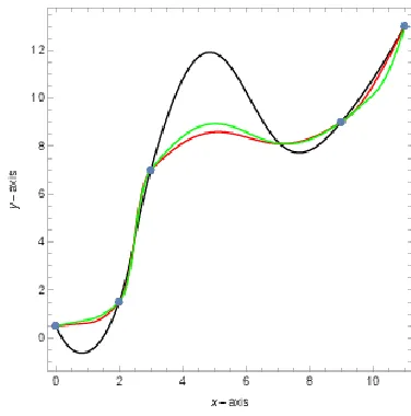
Data Table 1 is from Sarfraz [9]. The first derivative for Table 1 is calculated by using Equation [1-8].
Fig 1. The differences of derivative estimation
Fig 1 shows the interpolation curve between AMM (black), GMM (red) and HMM (green) derivative estimation method. From the figure, it can be concluded that the interpolation curve by using AMM derivative estimation gives the best curve compared with GMM and HMM.
3 R
ATIONALQ
UARTICS
CHEMEFor this paper, we are using the rational quartic scheme with different parameters such as Wang and Tan [10] and Zhu [13] schemes. These schemes will be compared with the proposed scheme of rational quartic spline with three parameters.
Wang and Tan [10] have been proposed the function of rational quartic spline with two parameters which are iand
i
as follow:
4063 ) ( ) ( ) ( ) ( ) ( t Q t p t s t h x s x s i i i i
i
(9) where 1 4 3 3 2 2 3 4 ) 1 ( ) 1 ( ) 1 ( ) 1 ( )
( i i i i i i
i t f t tA t t B t t V t f
p
t t Qi() i(1 ) i
With i i i i i
i f d h
V1 (3 ) ,V2 3i fi1 3ifiand
i i i i i
i f d h
V3 ( 3 ) 1 1 for iand i are shape parameters which will choose all positive and derivatives values given at knots xi.
Meanwhile, Zhu [13] constructed new rational quartic spline (quartic/cubic) with four parameters however, his scheme is too complicated and the derivation is difficult to understand. Let (xi fi) be given the real data and the derivative values
have been chosen at knots of xi where
b x x
x
a 1 2 ... n is partition of the interval [a,b]
forhi xi1 xi,
i i
h x x
t
, i i i i h f f 1
,Ai i di
and Bi di1 i
Then a new rational quartic interpolation spline given as
) ( ] ) 1 ( ) 1 ( )[ 1 ( ) 1 ( ) ( 2 1 2 1 t Q t B w t t B A t A w t h tf f t x s i i i i i i i i i i i (10)
where wi,i and i are the local tension shape parameters and 2 1 2 1 2 2 ) 1 )( ( ) 1 )( ( ) 1 ( )
(t w t B t t A t t w t
Qi i i i i i i i i
For the proposed scheme of rational quartic spline with three
parameters defined as for scalar
data{(xi, fi),i 0,1,..., n}wherex0 x1 ... xnand the first derivative di, at the respective pointxi,i0,1,..n. Then the
rational quartic spline with three parameters i,i 0 and 0
i
on the interval [xi,xi1],i0,1,..., n1 is given by:
) ( ) ( ) ( i i i Q P x S (11) where 1 4 3 2 2 3 4 ) 1 ( ) 1 ( ) 1 ( ) 1 ( )
( i i i i i i i
i f A B C f
p
2 2 ) 1 ( ) 1 ( )
( i i i
i
Q
2 2 1 4 3 2 2 3 4 ) 1 ( ) 1 ( ) 1 ( ) 1 ( ) 1 ( ) 1 ( ) ( i i i i i i i i i i i f C B A f x s (12)
The rational quartic spline defined by Equation (12) that satisfies the continuity
, ) ( , ) ( ) ( , ) ( 1 1 ) 1 ( ) 1 ( 1 1 ) 1 ( ) 1 ( i i i i i i i i d x s d x s f x s f x s (13) ) 1 (
s represents that the first derivatives of s with respect to x. Hences(x)C1[x0,xn]. By using the conditions in Equation (12) the unknowns’ coefficients Ai,Bi and Ci are determined
as follow are given by
1 1 1 ) 2 ( ) ( ) ( ) 2 ( i i i i i i i i i i i i i i i i i i i i i d h f C f f B d h f A (14) Data in Table 2 for comparison the curve for each rational quartic scheme for Fig 2.
TABLE2DATA POINTS FOR RATIONAL QUARTIC SCHEME
i
x 0 2 3 9 11
i
y 0.5 1.5 7 9 13
i
d -2.833 3.8333 4.7619 1.5833 2.4167
Fig 2 Comparison interpolation curve
Fig 2 shows the interpolation curve by schemes proposed scheme (blue), Wang and Tan [10] (red) and Zhu [13] (green). From figure above, it can be concluded that the curve interpolation for the proposed scheme gives more smoothness compared with the others scheme for data Table 2.
4 R
ESULT AND DISCUSSION4064 calculated error analysis for each example. For the proposed
scheme, we have selected three different values for each example. For each example, let assume that, f(x) for the true function for each example, p(x) is considered as the quartic polynomial. Other than that, Wang and Tan [10] scheme is considered as w(x) and z(x) for Zhu [13] scheme. Meanwhile, the proposed scheme is considered as s(x).
4.1 Example 1
Table 3 shows function of x
e x
f( ) for x{0,1,2,3,4}
Table 3: Data point
0 1 2 3 4
0 10 20 30 40 50
x axis
y
a
xi
s
( a ) Tr u e F u n c t i o n
( b ) Q u a r t i c P o l y n o mi a l
( c ) W a n g a n d Ta n [ 1 0 ]
( d ) Z h u [ 1 3 ]
( e ) T h e P r o p o s e d S c h e m e
( f ) T h e P r o p o s e d S c h e m e
Fig. 3 Interpolation curve i
x 0 1 2 3 4
i
y 1 2 . 7 1 8 2 3 7 . 3 8 9 1 2 0 . 0 8 5 5 5 4 . 5 9 8 2
i
4065 Fig 3 shows the interpolating curve for Example 1. Fig 3(a)
shows the interpolating the true value for the true function of x
e x
f( )
. Fig 3(b) shows the quartic polynomial with
2 , 1 ,
1
i i
i
. Fig 3(c) shows the interpolation curve by
scheme the Wang and Tan [10] and Figure 3(d) shows the Zhu [13] scheme. Fig 3(e) and Fig 3(f) show the interpolating
curve by the proposed scheme with three different value of i.
For Figure 3(e), the value parameter used
arei 1,i 1,i 0.03 meanwhile Figure 3(f), we used
3 . 0 , 1 ,
1
i i
i
. By using graphical estimation, Figure
3(e) shows smoothness visually to be compared with Figure 3(f).
TABLE 3FUNCTION VALUE FOR EXAMPLE 1
f(x) p(x) w(x) z(x) s1(x)
0.00 1.00000 1.00000 1.00000 1.00000 1.00000
0.20 1.22140 1.26370 1.21456 1.26864 1.22690
0.40 1.49182 1.58685 1.47887 1.58970 1.49676
0.60 1.82212 1.91699 1.81064 1.92304 1.81477
0.80 2.22554 2.26763 2.22087 2.27697 2.21838
1.00 2.71828 2.71828 2.71828 2.71828 2.71828
1.20 3.32012 3.43510 3.30153 3.42753 3.33507
1.40 4.05520 4.31351 4.01997 4.26838 4.06861
1.60 4.95303 5.21091 4.92182 5.17535 4.93305
1.80 6.04965 6.16405 6.03694 6.16983 6.03018
2.00 7.38906 7.38906 7.38906 7.38906 7.38906
2.20 9.02501 9.33758 8.97449 9.22757 9.06566
2.40 11.0231 11.7253 10.9274 11.4009 11.0596
2.60 13.4637 14.1647 13.3781 13.8641 13.4094
2.80 16.4446 16.7556 16.4101 16.6817 16.3917
3.00 20.0855 20.0855 20.0855 20.0855 20.0855
3.20 24.5325 25.3821 24.3951 24.8356 24.6430
3.40 29.9641 31.8728 29.7038 30.4996 30.0632
3.60 36.5982 38.5037 36.3676 37.1748 36.4505
3.80 44.7011 45.5465 44.6073 45.0740 44.5573
4.00 54.5981 54.5981 54.5981 54.5981 54.5981
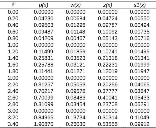
TABLE 4ABSOLUTE RELATIVE ERROR FOR TABLE 4
p(x) w(x) z(x) s1(x)
0.00 0.00000 0.00000 0.00000 0.00000
0.20 0.04230 0.00684 0.04724 0.00550
0.40 0.09503 0.01296 0.09787 0.00494
0.60 0.09487 0.01148 0.10092 0.00735
0.80 0.04209 0.00467 0.05143 0.00716
1.00 0.00000 0.00000 0.00000 0.00000
1.20 0.11499 0.01859 0.10741 0.01495
1.40 0.25831 0.03523 0.21318 0.01341
1.60 0.25788 0.03121 0.22231 0.01999
1.80 0.11441 0.01271 0.12019 0.01947
2.00 0.00000 0.00000 0.00000 0.00000
2.20 0.31257 0.05053 0.20256 0.04065
2.40 0.70217 0.09576 0.37777 0.03647
2.60 0.70099 0.08483 0.40041 0.05433
2.80 0.31099 0.03454 0.23708 0.05291
3.00 0.00000 0.00000 0.00000 0.00000
3.20 0.84965 0.13734 0.30314 0.11049
3.40 1.90870 0.26030 0.53555 0.09912
3.60 1.90548 0.23060 0.57659 0.14768
3.80 0.84535 0.09389 0.37282 0.14383
4.00 0.00000 0.00000 0.00000 0.00000
TABLE 5MAXIMUM VALUE FOR EXAMPLE 1
Scheme
Values of hi
05 . 0 i
h hi 0.1 hi 0.2
Quartic Polynomial p(x) 2.06935 2.06935 1.90869
Wang and Tan w(x) 0.26752 0.26451 0.26030
Zhu z(x) 0.58751 0.58374 0.57659
Quartic Spline
s1(x) 0.19317 0.19317 0.14768
s2(x) 0.51806 0.51806 0.51806
s3(x) 2.50076 2.50076 2.34859
Table 4 shows the function value for Example 1 while Table 5 shows the absolute relative error by using the value ofi 2 for the quartic polynomial,i 3for Wang and Tan
[10] scheme, i 3for Zhu [13] scheme
andi 0.03,i 0.3,i 3for the proposed scheme, s1(x) ,s2(x) and s3(x) respectively while the other parameters fixed to 1. Table 7.6 shows the maximum value for absolute relative error for various value forhi . From Table 6, it can be
concluded that the smallest of valuehi , the highest value of the maximum value for absolute relative error. For the proposed scheme, the s1(x) have the smallest value compare with others two. Value for hi 2 is more suitable for Example 1.
4066 From Fig 4, can be concluded that quartic polynomial the
highest value for the error compared with the other schemes.
Fig 5 Error interpolating curve for the proposed schemes
From Figure 5, the proposed scheme, s1(x) with value of 03
. 0 , 1 ,
1
i i
i
have the smallest absolute relative
error compare with s2(x) and s3(x).
4.2 Example 2
Data for Table 7 show function of
2 cos )
(x x
f for x= {0,
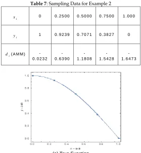
0.25, 0.5, 0.75, 1}. Table 7 shows the data points and derivative values using Arithmetic Mean Method (AMM).
Table 7: Sampling Data for Example 2
i
x 0 0 . 2 5 0 0 0 . 5 0 0 0 0 . 7 5 0 0 1 . 0 0 0
i
y 1 0 . 9 2 3 9 0 . 7 0 7 1 0 . 3 8 2 7 0
i
d ( A M M ) -0 . -0 2 3 2
-0 . 6 3 9 -0
-1 . -1 8 0 8
-1 . 5 4 2 8
-1 . 6 4 7 3
(a) True Function
(b) Quartic Polynomial
(c) Wang and Tan [10]
4067 (e) The Proposed Scheme
(f) The Proposed Scheme
Fig 6 Error interpolating curve for Example 1
Fig 6 shows the interpolating curve for Example 2. Fig 6(a) shows the interpolating of true function for Example 2. Figure
6(b) shows the quartic polynomial withi,i 1i 2. Fig
6(c) shows the Wang and Tan [10] scheme withi 1,i 5.
Fig 6(d) shows the Zhu [13] scheme
withi 1,i 1,i 0.5,ei 1. Fig 6(e) shows the
proposed scheme withi 1,i 1,i 0.05 .Figure 6(f)
shows the proposed scheme withi 1,i 1,i 0.5.
TABLE 8FUNCTION VALUE FOR EXAMPLE 2
f(x) p(x) w(x) z(x) s1(x)
0.0000 1.00000 1.0000 1.0000 1.0000 1.0000
0.0625 0.99518 0.9891 0.9925 0.9915 0.9950
0.1250 0.98079 0.9682 0.9775 0.9722 0.9802
0.1875 0.95694 0.9484 0.9555 0.9513 0.9566
0.2500 0.92388 0.9238 0.9238 0.9238 0.9238
0.3125 0.88192 0.8735 0.8902 0.8789 0.8818
0.3750 0.83147 0.8145 0.8412 0.8244 0.8310
0.4375 0.77301 0.7615 0.7771 0.7683 0.7726
0.5000 0.70711 0.7071 0.7071 0.7071 0.7071
0.5625 0.63439 0.6253 0.6524 0.6325 0.6344
0.6250 0.55557 0.5368 0.5769 0.5512 0.5552
0.6875 0.47140 0.4587 0.4803 0.4684 0.4710
0.7500 0.38268 0.3826 0.3826 0.3826 0.3826
0.8125 0.29028 0.2817 0.3152 0.2897 0.2905
0.8750 0.19509 0.1774 0.2246 0.1938 0.1949
0.9375 0.09802 0.0861 0.1105 0.0970 0.0977
1.0000 0.00000 0.0000 0.0000 0.0000 0.0000
TABLE 9ABSOLUTE RELATIVE ERROR FOR TABLE 8
p(x) w(x) z(x) s1(x)
0.00000 0.00000 0.00000 0.00000 0.00000
0.06250 0.00532 0.00607 0.00364 0.00019
0.12500 0.00945 0.01258 0.00855 0.00052
0.18750 0.00532 0.00849 0.00558 0.00030
0.25000 0.00000 0.00000 0.00000 0.00000
0.31250 0.00451 0.00817 0.00298 0.00005
0.37500 0.00801 0.01693 0.00699 0.00044
0.43750 0.00451 0.01142 0.00462 0.00036
0.50000 0.00000 0.00000 0.00000 0.00000
0.56250 0.00301 0.00902 0.00186 0.00009
0.62500 0.00535 0.01870 0.00437 0.00029
0.68750 0.00301 0.01262 0.00295 0.00036
0.75000 0.00000 0.00000 0.00000 0.00000
0.81250 0.00106 0.00850 0.00052 0.00022
0.87500 0.00188 0.01762 0.00128 0.00010
0.93750 0.00106 0.01189 0.00093 0.00031
1.00000 0.00000 0.00000 0.00000 0.00000
TABLE 10MAXIMUM ERROR FOR EXAMPLE 2
Scheme
Values of hi
05 . 0 i
h hi 0.1 hi 0.25
Quartic Polynomial p(x) 0.00945 0.00945 0.00945
Wang and Tan w(x) 0.03148 0.03148 0.02959
Zhu z(x) 0.00433 0.01408 0.01408
Quartic Spline
s1(x) 0.00053 0.00052 0.00052
s2(x) 0.00382 0.00382 0.00382
s3(x) 0.01348 0.01348 0.01347
Table 8 shows the function value for Example 2 while Table 9 shows the absolute relative error by using the value ofi 2 for the quartic polynomial,i 0.5 for Wang and Tan
10] scheme, i 0.5for Zhu [13] scheme
andi 0.05,i 0.5,i 5for the proposed scheme, s1(x)
,s2(x) and s3(x) respectively while the other parameters are
4068 Fig 7 Error interpolating curve for Example 2
Fig 8 Error curve interpolating for the proposed scheme
Fig 7 and Fig 8 show the error curve interpolating for Example 2.
4.3 Example 3
: The function of 2
3 ) 1 ( 1 )
(x x f
where,
] 4 , 0 [ , 3
1 k k x
is used. Table 11 shows the sampling
point for function 2
3 ) 1 ( 1 )
(x x f
.
TABLE 11SAMPLING POINT FOR EXAMPLE 3
i
x
0 . 3 3 3 3
0 . 5 0 0 0
0 . 6 6 6 7
0 . 8 3 3 3
1 1 . 1 6 6 7
1 . 3 3 3 3
1 . 5 1 . 6 6 6 7 i
y
0 . 7 5 4
0 . 6 3 4
0 . 5 5 7 2
0 . 5 1 4 0
0 . 5
0 . 5 1 4 0
0 . 5 5 7 2
0 . 6 3 4 0
0 . 7 5 4 6
( a ) Tr u e F u n c t i o n
( b ) Q u a r t i c P o l y n o mi a l
4069 ( d ) Z h u [ 1 3 ]
( e ) T h e P r o p o s e d S c h e m e
( f ) T h e P r o p o s e d S c h e m e
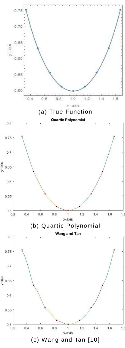
Fig 9 Interpolating curve for Example 3
Fig 9 shows the interpolating curve for Example 3. Fig 9(a) shows the interpolating curve for the true function. Figure 9(b) shows the curve for quartic polynomial with constant parameter i,i 1 i 2. Fig 9(c) shows the curve
interpolation scheme of Wang and Tan [10] by
usingi 1,i 2. As in Fig 9(c), the graph of interpolation
is not very smooth due to value of parameters. Fig 9(d) shows
the interpolating curve for Zhu [13] scheme. Fig 9(e) shows the proposed scheme withi 1,i 1,i 0.02 . Figure 9(f)
also shows the interpolating curve of the proposed scheme
with different values of
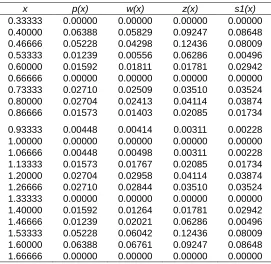
i . Figure 9(f) is by using the values of parameters of i 1,i 1,i 0.2TABLE 12FUNCTION VALUE FOR EXAMPLE 3
f(x) p(x) w(x) z(x) s1(x)
0.33333 0.75464 0.75464 0.75464 0.75464 0.75464
0.40000 0.70000 0.76388 0.75829 0.79247 0.78648
0.46666 0.65409 0.70637 0.69708 0.77845 0.73418
0.53333 0.61556 0.62796 0.62112 0.67843 0.62053
0.60000 0.58348 0.56757 0.56538 0.56568 0.55407
0.66666 0.55719 0.55719 0.55719 0.55719 0.55719
0.73333 0.53621 0.56331 0.56130 0.57131 0.57145
0.80000 0.52020 0.54724 0.54433 0.56134 0.55895
0.86666 0.50892 0.52466 0.52296 0.52977 0.52627
0.93333 0.50222 0.50670 0.50637 0.50534 0.50451
1.00000 0.50000 0.50000 0.50000 0.50000 0.50000
1.06666 0.50222 0.50670 0.50720 0.50534 0.50451
1.13333 0.50892 0.52466 0.52660 0.52977 0.52627
1.20000 0.52020 0.54724 0.54979 0.56134 0.55895
1.26666 0.53621 0.56331 0.56465 0.57131 0.57145
1.33333 0.55719 0.55719 0.55719 0.55719 0.55719
1.40000 0.58348 0.56757 0.57085 0.56568 0.55407
1.46666 0.61556 0.62796 0.63578 0.67843 0.62053
1.53333 0.65409 0.70637 0.71451 0.77845 0.73418
1.60000 0.70000 0.76388 0.76761 0.79247 0.78648
1.66666 0.75464 0.75464 0.75464 0.75464 0.75464
TABLE 13ABSOLUTE ERROR FOR EXAMPLE 3
x p(x) w(x) z(x) s1(x)
0.33333 0.00000 0.00000 0.00000 0.00000
0.40000 0.06388 0.05829 0.09247 0.08648
0.46666 0.05228 0.04298 0.12436 0.08009
0.53333 0.01239 0.00556 0.06286 0.00496
0.60000 0.01592 0.01811 0.01781 0.02942
0.66666 0.00000 0.00000 0.00000 0.00000
0.73333 0.02710 0.02509 0.03510 0.03524
0.80000 0.02704 0.02413 0.04114 0.03874
0.86666 0.01573 0.01403 0.02085 0.01734
0.93333 0.00448 0.00414 0.00311 0.00228
1.00000 0.00000 0.00000 0.00000 0.00000
1.06666 0.00448 0.00498 0.00311 0.00228
1.13333 0.01573 0.01767 0.02085 0.01734
1.20000 0.02704 0.02958 0.04114 0.03874
1.26666 0.02710 0.02844 0.03510 0.03524
1.33333 0.00000 0.00000 0.00000 0.00000
1.40000 0.01592 0.01264 0.01781 0.02942
1.46666 0.01239 0.02021 0.06286 0.00496
1.53333 0.05228 0.06042 0.12436 0.08009
1.60000 0.06388 0.06761 0.09247 0.08648
4070
TABLE 14MAXIMUM VALUE FOR ABSOLUTE RELATIVE ERROR
Scheme
Values of hi
5 . 0 . 0 i
h hi 0.1 hi 0.2
Quartic Polynomial p(x) 0.06609 0.06439 0.06388
Wang and Tan w(x) 0.07117 0.07072 0.06761
Zhu z(x) 0.12436 0.12436 0.12436
Quartic Spline
s1(x) 0.09645 0.09645 0.08648
s2(x) 0.09176 0.09176 0.08360
s3(x) 0.02878 0.02878 0.02771
Table 12 shows the function value for Example 3 while Table 13 shows the absolute relative error for proposed scheme and existing scheme by using the value ofi 2for the quartic
polynomial,i 2 for Wang and Tan [13] scheme, i 0.2 for
Zhu [13] scheme andi 0.02,i 0.2,i 20 for the proposed scheme, s1(x), s2(x) and s3(x) respectively while the other parameters are fixed to 1. From that table, it can be concluded that the highest value fori, the smallest value of absolute relative error. Table 14 shows the maximum value by different value ofhi. Forhi 0.0.5 , we can conclude that Zhu [13] have the highest value for maximum absolute relative error while the proposed scheme gives have the smallest value. For hi 0.0.5 andhi 0.1, the maximum value for Zhu [13] scheme and the proposed schemes of both value of
i
h are the same but is different for Wang and Tan [10] and
quartic polynomial.
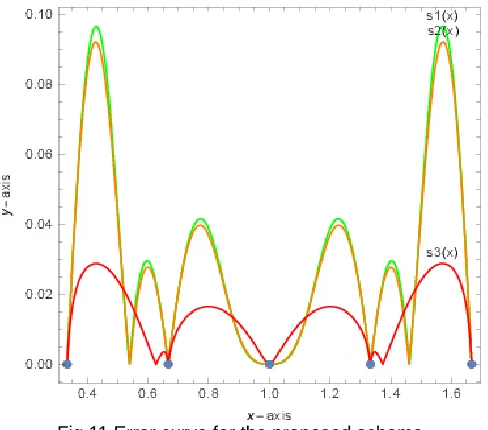
Figure 10 Error curve interpolating for example 3
Fig 11 Error curve for the proposed scheme
In Fig 10, it can be concluded that quartic polynomial and Wang and Tan [10] has the same value of absolute relative error and the highest error to be compared with the scheme by Zhu [13] and the proposed schemes. From Fig 11, we can tend to concluded that, the proposed scheme s3(x) withi 20 have the smallest error compared with the others parameters.
5 CONCLUSION
In this paper, a new rational fourth power spline (quartic/quadratic) with three parameters were created for curve and data interpolation. From the error analysis, it can be concluded that the proposed scheme with three parameters will implement for data interpolation by manipulating the values of parameters, it is able to do can the smallest error compare with the present schemes. We concluded that, the proposed scheme is more appropriate scheme compared to the existing schemes. For future studies, it will be more focusing on shape preserving interpolation by using the proposed scheme as well as image interpolation.
ACKNOWLEDGMENT
The author would like to acknowledge Universiti Teknologi Petronas (UTP) for the financial support received in the form
of a research grant: FRGS/
1/2018/STG06/UTP/03/1015MA0-020.
REFERENCES
[1] Brodlie, K. W., & Butt, S. (1991). Preserving convexity using piecewise cubic interpolation. Computers & Graphics, 15(1), 15-23
[2] Butt, S. and Brodlie, K.W. (1993). Preserving positivity using piecewise cubic interpolation. Computers & Graphics, 17(1), 55-64
[3] Delbourgo, A., & Gregory, J. A. (1984). The
determination of derivative parameters for a
4071
University Mathematics Technical Papers
collection;
[4] Delbourgo, R and Gregory, J.A (1985). The
determination of Derivative Parameters for a
monotonic Rational Quadratic Interpolant. IMA
Journal of Numerical Analysis, 5, 397-406.
[5] Delbourgo, R. (1989). Shape preserving interpolation to convex data by rational functions with quadratic numerator and linear denominator. IMA Journal of Numerical Analysis, 9(1), 123-136.
[6] Deng, S., Fang, K., Xie, J., & Chen, FJune). Rational biquartic interpolating surface based on function
values. In International Conference on
Technologies for E-Learning and Digital
Entertainment (pp. 773-780). Springer, Berlin,
Heidelberg
[7] Fritsch, F.N. and R.E. Carlson, 1980. Monotone
piecewise cubicinterpolation. SIAM J. Numer.
Analysis. 17: 238-246.
[8] Han, X (2008). Convexity-preserving piecewise
rational quartic interpolation. SIAM Journal of Numerical Analysis, 46(2), 920-929.
[9] Sarfraz, M., S. Butt, and M.Z. Hussain. (2001). Visualization of shaped data by a rational cubic spline interpolation. Computers & Graphics, 26,193-197.
[10]Wang, Q., & Tan, J. (2004). Rational quartic spline involving shape parameters. Journal of Information and Computational Science, 1(1), 127-130.
[11]Wang, Q., & Tan, J. (2006). Shape preserving piecewise rational biquartic surface. Journal of Information and Computational Science, 3, 295-302. [12]Wang, Y., Tan, J., Li, Z., & Bai, T. (2013). Weighted
rational quartic spline interpolation. Journal of Information & Computational Science, 10(9),
2651-2658.