Performance Evaluation of Bit Flipping and Sum Product Algorithm of LDPC coder in Different Channel Environment

(1)

IJEDR1402153

International Journal of Engineering Development and Research (www.ijedr.org)

2234

Performance Evaluation of Bit Flipping and Sum

Product Algorithm of LDPC coder in different

channel environment

1

Jigisha Patel,

2

Neeta Chapatwala,

3

Mrugesh Patel

1_{M E Scholar,}2_{Associate Professor,}3_Lecturer

Sarvajanik College of Engineering & Technology,, Surat, Gujarat, India.

[email protected], [email protected], [email protected]

________________________________________________________________________________________________________ Abstract— Low Density Parity Check (LDPC) codes are one of the block coding techniques that can approach the

Shannon’s limit within a fraction of a decibel for high block lengths. In many digital communication systems, these codes have strong competitors of turbo codes for error control. LDPC codes performance depends on the excellent design of parity check matrix and many diverse research methods have been used by different study groups to evaluate the performance. Unlike many other classes of codes, LDPC codes are already equipped with a fast, probabilistic decoding algorithm. This makes LDPC codes not only attractive from a theoretical point of view, but also very suitable for practical applications. This paper throws hard decision and soft decision algorithm of LDPC. The hard decision algorithm contains Bit flipping algorithm and Soft decoding algorithm contains Sum product algorithm which is used to correct burst error. Sum Product algorithm is also called as belief propagation. Bit flipping and Sum Product algorithms are explained and can be implemented for the generated parity check matrix of (648,324) for LDPC code with code rate 1/2.

Keywords- Encoder, Bit Flipping Algorithm, Sum Product Algorithm, AWGN, Rayleigh and Rician Channel

________________________________________________________________________________________________________

I.INTRODUCTION

Low-density parity-check (LDPC) codes are a class of linear block codes with implementable decoders, which provide near-capacity performance on a large set of data transmission and data-storage channels. Low-density parity-check (LDPC) codes were first introduced by R.G.Gallager[1] and rediscovered by MacKay in 1996[2]. Davey and Mackay rediscovered that by extending the order of Galois Field GF (q)[3]. This class of codes is known as non-binary LDPC codes. These codes are showing more and more competitive and have become some error-correcting code standards or the candidate standard in communication system.

LDPC codes were invented by Gallager in his 1960 doctoral dissertation and were mostly ignored during the 35 years that followed[2]. One notable exception is the important work of Tanner in 1981, in which Tanner generalized LDPC codes and introduced a graphical representation of LDPC codes, now called a Tanner graph[4]. The study of LDPC codes was resurrected in the mid 1990s with the work of MacKay, Luby, who noticed, apparently independently of Gallager’s work, the advantages of linear block codes with sparse (low-density) parity-check matrices[5].

The Bit-Flipping (BF) decoding algorithm[6], which was proposed by Gallager in 1962, and rediscovered by Mackay and Neal in 1996, is based on the hard decision of symbol. BF is simple and easy to be implemented, but has only limited decoding performance. Well designed LDPC codes decoded with iterative decoding based on belief propagation algorithm, such as the sum product algorithm (SPA)[7] achieve performance close to the Shannon limit 0.0045[8].

The paper is organized as follows: Section I the introduction of LDPC is explained. Section II is containing block diagram of the coded system. Section III is containing encoding method of LDPC for generating codeword that is transmitted on channel. Section IV decoding methods of LDPC in this section Bit Flipping (Hard Decision) and Sum Product (soft Decision) algorithm of the decoder is explained. Section V Results and analysis for different decoding algorithm explained. Section VI contains Conclusion.

II.BLOCK DIAGRAM OF CODED SYSTEM

(2)

IJEDR1402153

2235

Fig. I Coded System [2]

As shown in Fig. 1 encoder may encode user information by using encoding process of low density parity check (LDPC) code. The result of encoding user information is codeword denoted as w. Codeword may be of a predetermined length, which may be referred to as n, where n≥k. Codeword may include non-binary symbols corresponding to any of the elements in Galois Field (q), where q denotes the number of elements in the Galois Field. Codeword may be referred to as a GF (q) codeword.

Codeword is passed to a modulator. Modulator prepares codeword for transmission on channel. Modulator may use phase shift keying, frequency-shift keying, quadrature amplitude modulation, or any suitable modulation technique to modulate codeword into one or more information-carrying signals [2]. Channel may represent media through which the Information-carrying signals travel. For example, channel may represent a Wired or Wireless medium in a communication system.

Due to interference signals and other types of noise and phenomena, channel may corrupt the waveform transmitted by modulator. Thus, the waveform received by demodulator [1]. Received waveform may be different from the originally transmitted signal waveform. Received waveform may be demodulated with demodulator. The result of demodulation is received vector, which may contain errors due to channel corruption. Each entry in received vector may be referred to as a symbol or a variable. Each variable or symbol may be one of multiple non-binary values. Received vector may then be processed (decoded) by LDPC decoder. This processing may also equivalently be referred to as decoding a non-binary LDPC code or a received vector. LDPC decoder may be a non-binary code decoder. LDPC decoder may be used to correct or detect errors in received vector.

III.ENCODING

There are plenty of methods used for generating parity check matrix and Generator matrix. Parity check matrix is generated using Base matrix which consists of many sub matrices within it. Memory requirement is quite crucial issue during the VLSI implementation of LDPC codes. Generation of Parity check matrix using Base matrix requires less memory. Parity check matrix is obtained after expansion of Base matrix. Base matrix has elements like 0, -1 and any number between 0 to Z-1, where Z is an expansion factor. During expansion, -1 is replaced by Z x Z all zero matrix and any number between 0 to Z-1 is replaced by Z x Z identity matrix circular shifted by that number that shown in Fig. 2. Many of the standards like 802.11n, 802.16e etc. uses this method. Parity check matrix of size 324 x 648 is used for the simulation. Generator matrix is generated from parity check matrix using Gauss elimination method [5].

Fig. 2 Base matrix having expansion factor 7

A. Gauss Elimination Method

(3)

IJEDR1402153

2236

derived from the matrix multiplication c = u x G, where u is the message to be transmitted. The encoding process consists of normal matrix multiplication.

IV.DECODING ALGORITHM OF LDPC CODER

The algorithm used to decode LDPC codes was discovered independently several times and as a matter of fact comes under different names. The most common ones are the belief propagation algorithm, the message passing algorithm and the sum-product algorithm [7]. In order to explain this algorithm, a very simple variant which works with hard decision [6], will be introduced first. Later on the algorithm will be extended to work with soft decision which generally leads to better decoding results.

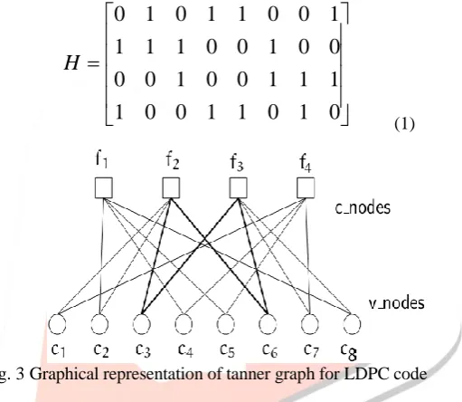
Tanner designed LDPC codes with a graphical representation method which called Tanner graph [4]. Tanner graph can express the decoding process of LDPC codes effectively and completely. For an example of Tanner graph with (8, 4) LDPC code is given in Figure 2 and it can describe a regular parity check matrix H intuitively in Eq. 1 Tanner graph has two different nodes which are the variable nodes (v-node) and the check nodes (c-node). Each row of a parity check matrix H is to match each check node of Tanner graph, and each column of a parity check matrix H is to match each variable node of Tanner graph. Check node i is connected to neighbor variable node j when hij in H is assigned to 1. Otherwise, it is not connected the value of this element is 0. Therefore, n variable nodes and m = n-k check nodes are existed in a parity check matrix H and are matched to Tanner graph.















0

1

0

1

0

1

0

1

0

1

0

1

0

1

0

1

0 H

(1)

Fig. 3 Graphical representation of tanner graph for LDPC code

A. Hard Decision (Bit Flipping) Algorithm

Here Hard Decision (Bit Flipping) Algorithm is explain by one example. An error free codeword of H is c = [1 0 0 1 0 1 0 1]. Suppose we receive y = [1 1 0 1 0 1 0 1]. So c2 was flipped. The algorithm is as follow

Step 1. All v-nodes ci send a”message” to their c-nodes fj containing the bit they believe to be the correct one for them. At this stage the only information a v-node ci is the corresponding received i

th

bit of c. That means for example, that c1 sends a message containing 1to f1 and f3, node c2 sends messages containing y1 (1) to f0and f1, and so on.

Step 2. Every check nodes calculate a response to their connected message nodes using the messages they receive from step 1. The response message in this case is the value (0 or 1) that the check node believes the message node has based on the information of other message nodes connected to that check node. This response is calculated using the parity-check equations which force all message nodes connect to a particular check node to sum to 0 (mod 2).

Table 1. Check nodes activities for hard-decision Decoder for code of Fig. 3

(4)

IJEDR1402153

2237

back to c5. At this point, if all the equations at all check nodes are satisfied, meaning the values that the check nodes calculate match the values that receive, the algorithm terminates. If not, we move on to step 3.

Step 3. In this step, the message nodes use the messages they get from the check nodes to decide if the bit at their position is a 0 or a 1 by majority rule. The message nodes then send this hard-decision to their connected check nodes. Table 2 illustrates this step. To make it clear, let us look at message node c2. It receives 2 0’s from check nodes f1 and f2. Together with what it already has y2 = 1, it decides that its real value is 0. It then sends this information back to check nodes f1 and f2.

Table 2. Message nodes decisions for hard decision Decoder for code of Fig. 3

Step 4. Repeat step 2 until either exit at step 2 or a certain number of iterations has been passed. In this example, the algorithm terminates right after the first iteration as all parity check equations have been satisfied. c2 is corrected to 0.

B. Soft-Decision Algorithm

The above description of hard-decision decoding was mainly for educational purpose to get an overview about the idea. Soft-decision decoding of LDPC codes [7], which is based on the concept of belief propagation, yields in a better decoding performance and is therefore belief propagation the preferred method.

The soft-decision decoder operates with the same principle as the hard-decision decoder, except that the messages are the conditional probability that the received bit is a 1 or a 0 given the received vector y.

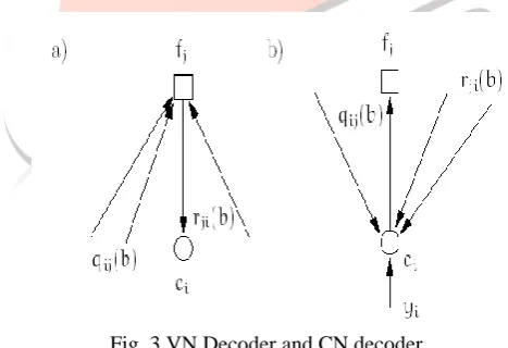
let Pi = Pr(ci = 1|yi) be the conditional probability that ci is a 1 given the value of y and let Pr(ci = 1|yi) = 1- Pi. qij is a message sent by the variable node ci to the check node fj. Every message contains always the pair qij(0) and qij (1) which stands for the amount of belief that yi is a”0” or a ”1”.

Fig. 3 VN Decoder and CN decoder

rji is a message sent by the check node fj to the variable node ci. Again there is a rji(0) and rji(1) that indicates the (current)amount of believe in that yi is a ”0” or a ”1”.The step numbers in the following description correspond to the hard decision case.

Step 1. All variable nodes send their qij messages to check node from below equation qij(1) = Pi and qij(0) =1 - Pi (2)

Step 2. The check nodes calculate their response messages rji

 

_













i j

j i ji

v i

q

r

/

'

)

1 (

2

1

2

1

2

1

0

(3)

(5)

IJEDR1402153

2238

)

0 (

1 )

1 (

ji ji

r





₍₄₎

So they calculate the probability that there is an even number of 1’s among the variable nodes except ci (this is exactly what Vj\i means). This probability is equal to the probability rji(0)that ci is a 0. This step and the information used to calculate the responses is illustrated in Fig. 3.

Step 3. The variable nodes update their response messages to the check node ci to the variable node fj. This is done according to the following equations,









j i i j ij ij c j

r

Pi

k

q

/ ' '

)

0 (

)

1 (

)

0 (

(5)







j i i j i ij ij c j

r

P

k

q

/ ' '

)

0 (

)

1 (

(6)

Where by the Constants Kij are chosen in a way to ensure that qij(0)+qij(1) = 1. Ci\j now means all check nodes except fj.At this point the v-nodes also update their current estimation their variable ci. This is done by calculating the probabilities for 0 and 1 and voting for the bigger one. The used equations are quite similar to the ones to compute qij(b) but now the information from every c-node is used.









i ji i i i C j

r

P

K

Q

(

0 )

(

1 )

(

0 )

(7)







i ji i i i C j

r

P

K

Q

(

1 )

(

1 )

(8)

If the current estimated codeword fulfills now the parity check equations the algorithm terminates. Otherwise termination is ensured through a maximum number of iterations.

(9)

V.RESULTSANDANALYSIS

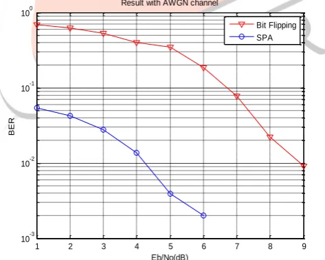
In this section, the BER performance for the Hard decision (Bit flipping) and Soft decision (Sum Product) algorithms with irregular (324,648)LDPC codes with codeword length is 648 and code rate is 0.5 are implemented. The simulations are performed over an additive white Gaussian noise (AWGN), Rayleigh and Rician channel with BPSK modulation.

1 2 3 4 5 6 7 8 9

10-3 10-2 10-1 100 Eb/No(dB) BER

Result with AWGN channel

Bit Flipping SPA

Fig. 4 Simulation result for BF and SPA algorithm for AWGN channel

















else

Q

ifQ

C

i i i

(6)

IJEDR1402153

2239

1 2 3 4 5 6 7 8 10-3

10-2 10-1 100

Eb/No(dB)

BER

Result with rician channel

Bitflipping SPA

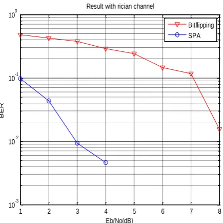
Fig. 5 Simulation result for BF and SPA algorithm for Rician channel

1 2 3 4 5 6 7 8

10-3 10-2 10-1 100

Eb/No(dB)

BER

Result with rayleigh channel

Bitflipping SPA

Fig. 6 Simulation result for BF and SPA algorithm for Rayleigh channel

Fig. 4, Fig. 5 and Fig. 6 are shows BER Vs SNR is plotted for the Hard decision (Bit flipping) and Soft decision (Sum Product) algorithms for the different channel environment. BER performance of the soft decision (SPA) algorithm is improves by compare hard decision (BFA). For Rician channel BER performance of both algorithm is improve by comparing with AWGN and Rayleigh channel.

VI.CONCLUSIONS

BER Performance for Sum Product Algorithm and Bit Flipping Algorithm is checked with different channel environment. It is observed that for Rician channel BER performance of both algorithm is improve as comparing with AWGN and Rayleigh channel. It can be seen from BER performance that the Sum Product Algorithm is better in comparison with Bit flipping Algorithm.

ACKNOWLEDGEMENT

I am really thankful to my guide without which the accomplishment of the task would have never been possible. I am also thankful to all other helpful people for providing me relevant information and necessary clarifications.

REFERENCES

[1] William E. Ryan, Shu Lin, “Channel Codes-Classical and Modern”,Cambridge University Press 2009, ISBN-13 978-0-511-64182-4 eBook (NetLibrary).

[2] R.G. Gallager, “Low-density parity check codes,” IRE Transaction Info.Theory, vol. IT-8, pp. 21–28, Jan. 1962.

[3] S.-Y. Chung, D. Forney, T. Richardson, and R. Urbanke, “On the design of low-density parity-check codes within 0.0045 dB of the Shannon limit," IEEE Communication Letters, vol. 5, pp. 58 − 60, 2001.

(7)

IJEDR1402153

2240

[5] S. K. Chilappagari, B. Vasi´c, and M. W. Marcellin, “Guaranteed error correction capability of codes on graphs,” in

Proceedings of the Information Theory and Applications, UCSD, Feb. 8 - 13, 2009.

[6] D. Burshtein, “On the error correction of regular LDPC codes using the flipping algorithm,” IEEE Trans. Inf. Theory, vol. 54, no. 2, pp.517–530,Feb. 2008.

[7] T. Richardson and R. Urbanke, “The capacity of low-density parity check codes under messagepassing decoding,” IEEE Trans. Inform. Theory, vol. 47, pp. 599 – 618, 2001.

[8] Lingqi Zeng, Ying Y. Tai, Member, IEEE, Lei Chen, Shu Lin,Life Fellow, IEEE, and Khaled Abdel-Ghaffar, Member, IEEE ,“Construction of Quasi-Cyclic LDPC Codes for AWGN and Binary Erasure Channels: A Finite Field Approach” , IEEE Transactions On Information Theory, Vol. 53, No. 7, July 2007.

[9] David declercq, marc fossorier, fellow, “Decoding algorithms for non binary ldpc codes over gf(q),” IEEE transactions on communications, vol. 55, no. 4,pp.633,643, april 2007.