FOREIGN AID, GOVERNMENT EXPENDITURE AND
SECTORAL GDP GROWTH IN KENYA
KENNETH KIBET LAGAT
K102/CTY/PT/20611/2010
A Research Project Submitted to the Department of Economic Theory in the School of
Economics in partial fulfillment of the requirements for the award of the Degree of
Master of Economics (Policy and Management) of Kenyatta University
i
DECLARATION
This research project is my original work and has not been presented for a degree or any other award in any University.
Signature: ... Date: ... Kenneth Kibet Lagat
BA (Hon) in Economics & Mathematics Reg. No. K102/CTY/PT/20611/2010
This research project was submitted for examination with our approval as University Supervisors.
Signature: ... Date: ... Dr. George Kosimbei
Senior Lecturer
Department of Economic Theory Kenyatta University
Signature: ... Date: ... Dr. Steve Makori
Lecturer
ii
DEDICATION
iii
ACKNOWLEDGEMENTS
First and foremost, I wish to express my sincere gratitude to the ALMIGHY GOD. To Him, be the glory and honour. I would like to express my gratitude to my supervisors, Dr.George Kosimbei and Dr. Steve Makori for their constructive recommendations, suggestions, criticisms and advice which were invaluable in shaping this project. I am also grateful to those who may have been involved in different ways including moral, financial and spiritual support in the course of this study. I would like to express my gratitude to the National Treasury, in particular the Director of External Resources Department, for the scholarship to undertake the master’s programme at Kenyatta University.
Special gratitude goes to my wife Eddah Waihiga Maina and my daughter Maria Jerop Lagat for the unending support, love and encouragement which have gotten me this far. I owe a lot of appreciation to my friends whose comments and criticisms added value to this project. Specifically, I would like to acknowledge comments and encouragement received from Abel Otwori, Parliamentary Budget Office and George kariuki, Kenyatta University.
iv
TABLE OF CONTENTS
DECLARATION ... i
DEDICATION ... ii
ACKNOWLEDGEMENTS ... iii
OPERATIONAL DEFINITIONS OF TERMS ... viii
ABBREVIATIONS AND ACRONYMS ... x
ABSTRACT ... xi
CHAPTER ONE: INTRODUCTION ... 1
1.1 Background ... 1
1.2 Problem Statement ... 10
1.3 Research Questions ... 11
1.4 Objectives of the study ... 11
1.5 Significance of the study ... 12
1.6 Scope of the study ... 12
CHAPTER TWO: LITERATURE REVIEW ... 13
2.1 Introduction ... 13
2.2 Theoretical Literature ... 13
2.3 Empirical Literature ... 21
2.4 Overview of Literature ... 27
CHAPTER THREE: METHODOLOGY ... 29
3.1 Introduction ... 29
3.2 Research Design ... 29
3.3 Theoretical Framework ... 29
3.4 Model Specification ... 31
3.5 Definition and measurement of variables ... 32
3.6 Data types and sources ... 33
3.7 Panel data Properties ... 33
3.8 Data Analysis ... 34
CHAPTER FOUR: EMPIRICAL FINDINGS ... 35
4.1 Introduction ... 35
4.3 Panel data Properties ... 36
v
CHAPTER FIVE: SUMMARY, CONCLUSION AND POLICY RECOMMENDATIONS
... 44
5.1 Introduction ... 44
5.2 Summary ... 44
5.3 Conclusion... 45
5.4 Policy Recommendations ... 46
5.5 Limitations ... 47
5.6 Areas of future research ... 47
REFERENCES ... 49
vi
LIST OF TABLES
Table 3. 1: Definition and measurement of variables ... 32
Table 4. 1: Descriptive Statistics for the Panel……….……...……..35
Table 4. 2: Results from Unit Root Test ... 37
Table 4. 3: Hausman test results ... 38
Table 4. 4: Regression results ... 39
Table A 1: Sectoral GDP growth and Contributions to sectoral GDP (in Constant and Current prices)………..…………..……....53
vii
LIST OF FIGURES
Figure 1. 1: Foreign aid, Government expenditure and sectoral GDP growth (Health sector) . 6
Figure 1. 2: Foreign aid, Government expenditure and sectoral GDP growth (Agriculture and forestry sector) ... 7
Figure 1. 3: Foreign aid, Government expenditure and sectoral GDP growth (Education sector) ... 9
viii
OPERATIONAL DEFINITIONS OF TERMS
Development Expenditure: Total of expenditures from all the development projects and activities carried out by Government Ministries, Departments and Agencies.
Economic growth: Refers to the increase in the economy’s output over time. It is measured using real GDP in constant prices due to the fact that changes over time in GDP in current prices are as a result of a mixture of price changes and output changes.
Employment: A contract between two parties, where one party is working in a full time or part time basis in exchange for compensation, either in the public or non-public (private) sector.
Foreign aid: Refers to aid flows to developing countries which are provided by official agencies, and each transaction of which is administered with the promotion of the economic development and welfare of developing countries as its main objective. It includes grants but excludes loans.
Foreign Aid (Appropriation in Aid): Refers to aid flows that are factored in the annual budget and disbursed directly to the implementing entity.
Foreign Aid (Revenue): Refers to aid flows that are factored in the annual budget and disbursed through the government disbursement systems.
Government expenditure: Refers to the amount spent on personnel remuneration, goods and services and on capital investments by the government. It comprises of development expenditure and recurrent expenditure.
ix
Recurrent expenditure: refers to those expenditures which are undertaken by the Ministries, Departments and Agencies (MDAs) to cover day-to-day normal services, wages and salaries (labour costs) and operation and maintenance along with minor capital expenditures such as purchase of equipment.
Sectoral Gross domestic product (sectoral GDP): It is the total value of all goods and services produced over a given time period in a given sector of an economy.
x
ABBREVIATIONS AND ACRONYMS
AIA Appropriation in Aid
ARDL Autoregressive Distributive Lag
DPs Development Partners
GDP Gross Domestic Product
GLS Generalized Least Square Method
IPS Im-Pesaran-Shin test
KNBS Kenya National Bureau of Statistics
Kshs Kenya Shillings
LLC Levin-Lin-Chu test
MDAs Ministries, Departments and Agencies
MDGs Millennium Development Goals
MTEF Medium Term Expenditure Framework
NARC National Alliance of Rainbow Coalition
NT National Treasury
ODA Official Development Assistance
OECD Organization for Economic Co-operation and Development
OLS Ordinary Least Square Method
PFM Public Financial Management
SAPs Structural Adjustment Programmes
UNDP United Nations Development Programme
xi
ABSTRACT
1
CHAPTER ONE
INTRODUCTION
1.1 Background
Government play important roles in any modern economy such as promotion of economic growth, employment creation, ensuring efficiency in allocation of resources and stabilization of the economy by spending resources that are mobilised domestically through tax revenues and from external resources in form of foreign aid. However the roles of foreign aid and government expenditure in fostering economic growth and development continue to be contentious debates among policy makers and researchers (Gomanee, K., Girma S., and O. Morrissey ,2005; Nyagwachi, 2013).
Foreign aid flows began during and after the World War II, when it was used primarily to support the rebuilding of economies of Western Europe and contain the Soviet expansion in the aftermath of World War II through the famous Marshall Plan. The Marshal plan was widely considered as a great success with many European countries undergoing a period of rapid industrialization during the late 1940s and early 1950s. Following the success of the Marshal plan, US president Harry Truman announced a major programme of increased foreign assistance to the developing countries in 1949 (Rotarou and Ueta, 2009; Tarp, 2009). According to Tarp (2009), it is after the success of the Marshall Plan, that the attention of industrialized nations turned to the developing countries, many of which became independent during the 1960s, with the belief that poverty and inequality in these countries would be quickly eliminated through growth and modernization.
2
one was to promote short-term political and strategic interests of donor countries (World Bank, 1998). Despite the increased flow of foreign aid, the continent still face development challenges especially with regard to meeting the Millennium Development Goals (MDGs), (Gomanee et. al, 2005).
The concern on the effectiveness and efficiency of foreign aid has resulted in several meetings aimed at improving aid effectiveness. These include the Monterrey Consensus on Financing for Development in 2002, (United Nations, 2003); the Rome Declaration on Harmonization in 2003; the Paris Declaration in 2005 (OECD, 2005); Accra Agenda for Action in 2008 (OECD, 2008) and the Busan Partnership for effective Development in 2012 (OECD, 2012). The Monterrey consensus resolved to address the challenges of financing for development around the world and developing countries especially those needed to attain the MDGs. Furthermore, it emphasized the need of scaling up foreign aid as one of the important financing tools to achieve the new development goals (United Nations, 2003). In the same breath, the Commission for Africa (2005) argued for a substantial increase in resources for SSA, especially to finance needed investment, estimated as requiring an additional US$25 billion per annum in aid to Africa to be achieved by 2010, with a further US$25 billion per annum increase by 2015.
1.1.1 Overview of Foreign Aid, Government expenditure and Economic performance in
Kenya
3
a remarkable growth rate, about 6.5 percent annually, attributed to both high flows of foreign investment and technical assistance.
During the first two decades after independence, both bilateral and multilateral aid sources were many and increasing. Gross ODA inflows increased from an annual average of US$205 million in the 1970s to US$630 million in the 1980s and slightly over US$1 billion in the 1990s. This is partly attributed to the flows arising from the need to cushion the economy from the effects of the SAPs and the need to ensure sustenance of the reforms that the country was undertaking during the period. Thereafter, the flow of aid assumed a declining trend due to the persistent aid cuts in the 1990s and 2000s. The period 2001-2011 recorded some growth in ODA flows mainly from the multilateral donors compared to the previous period. This could be attributed to the increased donor interest in Kenya arising from the regime change in 2002 and Kenya’s commitment to reform. (Njeru, 2003; Ojiambo, 2009).
Kenya’s economy performed remarkably well in the 1960s and early 1970s, registering an average of 6.6 percent annual growth in GDP during 1964-73. However, this growth was not sustained mainly due to exogenous factors. During 1974-79, the growth rate declined to 5.2 percent, dropping even further to 4.1 percent over 1980-89 and down to 2.5 percent in 1990-95. The annual GDP growth rate continued to decline reaching a low of 1.4 percent in 1999, 0.6 percent in 2000 and it rose to 4.4 percent in 2001; however it fell again to a low 0.5 percent in 2002. Some of the reasons behind poor economic performance include reduced investor confidence, poor governance, institutionalized corruption, poor infrastructure, reduced inflows of donor assistance, and unfavorable weather conditions (Republic of Kenya and UNON, 2003).
4
over the period despite adverse effects of drought and high oil prices (Republic of Kenya and UNDP Kenya, 2012). Growth dropped from 7.1 percent in 2007 to 1.6 percent in 2008, before reaching 2.6 percent in 2009 reflecting a moderately strong recovery in view of the global economic crisis at the time, (World Bank, 2010). Real GDP expanded by 5.6 percent in 2010 compared to a growth of 2.6 percent in 2009 whereas Real GDP expanded by 4.6 percent in 2012 compared to a growth of 4.4 percent in 2011 ( World Bank, 2011; 2012;2013).
The Government of Kenya undertook some key macroeconomic reforms such as Public Financial Management reform and long-term planning such as the Vision 2030. An efficient PFM system was thought to be a key factor to efficient utilization of scarce public resources, foreign aid included. On the other hand, Vision 2030 aims at transforming Kenya into a globally competitive and prosperous country with a high quality of life. The vision is anchored on the following three pillars; the Economic pillar, the Social pillarand the Political pillar. The blueprint also identifies some key sectors that will play the key role of delivering the GDP growth of 10 percent and propelling the country into middle income economy. These sectors include agriculture, health, and education among others (Republic of Kenya, 2007).
5
6
Figure 1. 1: Foreign aid, Government expenditure and sectoral GDP growth (Health sector)
Source of data: Various NT Development Estimates and variousKNBS Statistical Abstracts
The health sector experienced a high growth rate of 27.2 percent in 1996 and a negative growth rate of -0.6 percent 1991. From 2002, the aid flows to the health sector as a percentage of health GDP increased from 8.71 percent in 2002 to 24.56 percent in 2007. The government expenditure as a percentage of health GDP increased from 54.67 percent in 2002 to 94.88 percent in 2007, however, the GDP growth rates for the sector kept on fluctuating.
The total government expenditure and foreign aid flows to the agriculture and forestry sector as a percentage of the agriculture real GDP have been low relative to the health and education sectors. The sector managed a higher rate of government expenditure of 16.2 percent in 2012 and lower rates of 0.2 percent and 0.3 percent in 1991 and 1992 respectively. This also
-20% 0% 20% 40% 60% 80% 100% 120% 140% 160% 180% 200%
1980 1981 1982 1983 1984 1985 1986 1987 1988 1989 1990 1991 1992 1993 1994 1995 1996 1997 1998 1999 2000 2001 2002 2003 2004 2005 2006 2007 2008 2009 2010 2011 2012
7
corresponded with a decline in the growth rate of the sector from 3.50 percent in 1990 to -0.90 percent in 1991 to -3.60 percent in 1992 as illustrated in figure 1.2 below.
Figure 1. 2: Foreign aid, Government expenditure and sectoral GDP growth (Agriculture and forestry sector)
Source of data: Various NT Development Estimates and variousKNBS Statistical Abstracts
The decline in government expenditure and foreign aid flows as a share of agriculture and forestry real GDP together with the low growth rates could be attributed to drop in the aid flows to the sector following the aid freeze to Kenya. Furthermore, Kenya had her first general election under a multi-party system at that time, which meant government resources
-10% -5% 0% 5% 10% 15% 20% 198 0 198 1 198 2 198 3 198 4 198 5 198 6 198 7 198 8 198 9 199 0 199 1 199 2 199 3 199 4 199 5 199 6 199 7 199 8 199 9 200 0 200 1 200 2 200 3 200 4 200 5 200 6 200 7 200 8 200 9 201 0 201 1 201 2
Foreign aid flows to Agriculture & Forestry sector (As a percentage of sector real GDP)
Government Expenditure to Agriculture & Forestry sector (As a percentage of the sector real GDP)
8
were being diverted from the agriculture and forestry sector to the social sectors, in this regard the education and health sector.
The sector experienced a higher growth rate of 10.5 percent in 2001, however it also experienced negative growth rates of -3.6 percent, -0.9 percent, -3.6 percent, -3.8 percent, -3.2 percent, -1.2 percent, -3.1 percent,-4.1 percent and -2.6 percent in 1984, 1991, 1992, 1993, 1997, 2000, 2002, 2008 and 2009 respectively. The decline in the real GDP growth in the sector in the stated years could be attributed to high prices of inputs, adverse weather conditions and disruption from the post-election violence in 2008. The decline in 2009 could be explained by depressed demand in the international market especially for horticultural produce.
The education sector experienced an increasing trend in foreign aid flows and government expenditure as a percentage of real GDP in the education sector with exception of 1992 and 1997, when the foreign aid flows declined from 1.25 percent in 1991 to 1.15 percent in 1992 and from 1.59 percent in 1996 to 1.48 percent in 1997. The education growth rates also declined from 10.0 percent in 1991 to 4.7 percent in 1992 and from 7.7 percent in 1996 to 2.2 percent in 1997 as shown in figure.1.3 below.
9
programme that started under the NARC regime. In the year 2011 and 2012, the increasing trend in foreign aid flows to the sector’s GDP continued after the government took bold steps in prosecuting the corrupt officials who misappropriated the donor funds in the Ministry of Education.
Figure 1. 3: Foreign aid, Government expenditure and sectoral GDP growth (Education sector)
Source of data: Various NT Development Estimates and variousKNBS Statistical Abstracts
-10% -5% 0% 5% 10% 15% 20% 25% 0% 50% 100% 150% 200% 250% 1 9 8 0 1 9 8 1 1 9 8 2 1 9 8 3 1 9 8 4 1 9 8 5 1 9 8 6 1 9 8 7 1 9 8 8 1 9 8 9 1 9 9 0 1 9 9 1 1 9 9 2 1 9 9 3 1 9 9 4 1 9 9 5 1 9 9 6 1 9 9 7 1 9 9 8 1 9 9 9 2 0 0 0 2 0 0 1 2 0 0 2 2 0 0 3 2 0 0 4 2 0 0 5 2 0 0 6 2 0 0 7 2 0 0 8 2 0 0 9 2 0 1 0 2 0 1 1 2 0 1 2
Foreign aid flows to Education sector ( As a Percentage of Education real GDP)-Left Axis
Government Expenditure to Education sector ( As a percentage of education real GDP)-Left Axis
10
1.2 Problem Statement
Kenya has been a recipient of Foreign aid since she gained her independence in 1963. Official foreign aid to developing countries such as Kenya is always issued to governments to fund government spending especially development expenditure (Gomanee et. Al, 2005). However the roles of foreign aid and government expenditure in fostering economic growth in Kenya have not been explored exhaustively. Several studies have been done on foreign aid-growth nexus in Kenya for example Njeru (2003); M’Amanja and Morrissey (2006); Ojiambo (2009), and on government expenditure-growth nexus in Kenya for example, Maingi (2010); M’Amanja and Morrissey (2005); Muthui et. al (2013); Ojwang (2013). These studies analysed the entire economy, however there are no studies carried out to establish the aid-growth nexus at the sectoral level and there are very limited studies carried out to establish government expenditure-growth nexus at sectoral level for example Nyagwachi, (2013). This study focussed on the effects of government expenditure and wage employment on sectoral growth but did not consider the effects of foreign aid on sectoral GDP growth in Kenya.
The Kenyan government spends resources that are mobilised through domestic revenue collections and from external resources in the form of aid flows, in order to stimulate and sustain economic growth, invest in infrastructure, agriculture and forestry and to deliver key services such as health, education, which could otherwise be expensive if left to the private sector.
11
aid flows and government expenditure to the three sectors increasing both in absolute terms and as a percentage of the real sectoral GDP, as indicated in figures 1.1, 1.2 and 1.3.
This study therefore sought to investigate and fill the gap in literature of whether foreign aid and government expenditure enhance, deter or have no impact on sectoral GDP growth in Kenya, based on the fact that it has not been adequately covered by other studies.
1.3 Research Questions
This research study sought to address the following questions:
i. What are the effects of foreign aid on sectoral GDP growth in Kenya?
ii. What are the effects of government development expenditure on sectoral GDP growth in Kenya?
iii. What are the effects of government recurrent expenditure on sectoral growth in Kenya?
1.4 Objectives of the study
1.4.1 General Objective
The general objective of this study was to determine the effects of foreign aid and government expenditure in agriculture and forestry, education and health on GDP growth in the sectors.
1.4.2 Specific Objectives
i. Determine the effects of foreign aid on sectoral GDP growth in Kenya
ii. Determine the effects of government development expenditure on sectoral GDP growth in Kenya
12
1.5 Significance of the study
This study will help policy makers in decision making especially when it comes to mobilization of foreign aid and allocation of scarce budgetary resources in agriculture and forestry, education and health sectors in light of the devolved system of governance. This study will also provide guidance to policy makers in Kenya at the National and sectoral level on effects of foreign aid and government expenditure on the economic performance of the above sectors.
1.6 Scope of the study
13
CHAPTER TWO
LITERATURE REVIEW
2.1 Introduction
This chapter presents both the theoretical and empirical literature on the Foreign aid-sectoral GDP growth nexus and government expenditure-sectoral GDP growth nexus.
2.2 Theoretical Literature
Foreign Aid and Economic growth
2.2.1 The Two Gap Model
Two Gap Model was advanced by Chenery and Strout (1966) to predict the macroeconomic impact of foreign aid. The two-gap model combined three model strains for estimating macroeconomic impact of foreign aid. The strains are: the skill limitation (essentially the capital absorptive capacity approach); the gap between domestic investment required to achieve a givenrate of economic growth and domestic savings and the gap between foreign exchange requirements to sustain the required level of domestic investment and the country's foreign exchange earnings.
According to Harms and Lutz (2004), the two gap model has two components. The first component is the relationship between investment and growth, wherein the level of growth is assumed to be dependent on the level of investment. The model is based on the Harrod-Domar model which assumes a linear relationship between output (Y) and capital (K),
Y=𝐾𝑣,………... (2.1)
14
𝑌̇ 𝑌 =
𝐾̇
𝑣𝑌=
𝐼
𝑣𝑌 - 𝛿, ………. (2.2)
where a dot over a variable denotes the change over time (e.g. 𝑌̇ = 𝑑𝑌
𝑑𝑡 is the change in output
between now and the next period) and δ the depreciation rate. Note that current output is
predetermined by past investments. As a planning framework, (2.2) allow policy makers to determine the minimum level of investment (I*) required to achieve the desired rate of output growth (g*):
𝐼∗
𝑌 = v (g* +𝛿), ………. (2.3)
The second component is the relationship between savings, which is assumed as a critical factor for investment expansion and growth. From basic national income accounting we know that
Sp− I = (G − T) + (X− M) ………..…………... (2.4)
where Sp= private savings, G = government (current and capital) expenditure, T = taxes, X =
exports and M = imports. Equation (4) can be rewritten as
I = 𝑆𝑝 + (𝑇 − 𝐺)⏟
Domestic savings
+ (𝑀 − 𝑋) ⏟
Foreign savings
= S+F……… (2.5)
In equation (2.5), private savings and the budget surplus have been aggregated into ‘domestic savings’ (S). The last term is referred to as ‘foreign savings’ (F), since the trade
deficit (on goods and services) has to equal the sum of net current transfers (including foreign aid), net capital inflows (capital account plus financial account) and net factor payments.
15
I SG≤ S + F…………... (2.6)
If the resulting investment level happens to be below the desired level I*, the economy would be facing a savings gap. To derive the foreign-exchange gap, the model assumes further that imports consist of capital imports (MK) and other imports (MO):
M = MO+ MK.………. (2.7)
A fixed share m of all capital goods needs to be imported from abroad,
I = 1
𝑚MK =
1
𝑚 (M-MO)………...(2.8)
Substituting M = X + F into this equation gives
I = 𝑚1[(X – MO) + F] ………. (2.9)
Again, the two-gap model assumes that the variables on the right-hand side are either exogenous or predetermined. The investment constraint due to this foreign-exchange restriction is given by
IFG≤𝑚1[(X – MO) + F]………... (2.10)
There is a ‘foreign exchange gap’ (or ‘trade gap’), if this investment level is below I*, i.e.
below the level required to achieve the desired level of output growth g*.
Depending on the various exogenous and predetermined variables, either the savings constraint (2.6) or the foreign-exchange constraint (2.10) can be binding for a country. In this regard, the role of foreign aid is to supplement the savings gap and the foreign exchange gap.
16
The two gap model is not without criticism, especially with regard to its assumptions. Harms and Lutz (2004) point out that the gap model laid more emphasis on the role of physical capital investment, without paying attention to other determinants of growth such as education and research & development. Harms and Lutz (2004) also argue that in reality, domestic recipient of aid is either the government or part of the public sector. In this regard, it is possible that it alters its general expenditure pattern as a result of the foreign aid inflow. For instance, resources previously earmarked for investment may get re-allocated to recurrent expenditure.
2.2.2 The Solow-Swan Model and the Poverty Traps
According to Barro and Sala-i-Martin (2004), the Solow–Swan model is a simple neoclassical growth model which supposes that all the assumptions of the Solow model are satisfied; that is the function F (.) exhibit constant returns to scale:
F (λK, λL) =λ. F (K, L), for all λ >0 ……….... (2.11)
The model further assumes that there are no private international capital flows, such that domestic investment I has to be financed out of domestic savings S. It postulates that growth of per-capita output is the result of capital accumulation and/or technological progress. As soon as the economy reaches its steady state, per-capita output growth is only possible via technological progress, which is exogenous in the model (Harm and Lutz, 2004). According to Harm and Lutz (2004),
Y=F (K, L); K̇ = I −δK; I=S, ………... (2.12) where δ denotes the exogenous rate of depreciation.
17
income doesn’t exceed this level of consumption. Thus the savings function can be described
as follows.
S= {s[Y − C̃L] if Y > C̃L
0 if Y ≤ C̃L , ……….…... (2.13)
with 0 < s < 1 and C̃ representing per capita consumption needs.
If we combine equations (2.12) to (2.14), we obtain a modified ‘Solow equation’:
k̇ = s[f(k) − C̃] – (δ + n)k, ………...……...…... (2.15)
where k is the capita stock in per-capita terms and n is the exogenous population growth rate.
In figure 2.1 below, the evolution of capital stock, k̇ is depicted as the vertical distance
between s[f(k) − C̃] and (δ + n) k. The figure above has two steady states: one stable,
Solow-type steady k∗∗, and the second one, unstable steady state, k∗ that determines the boundary of the poverty trap. If a country’s initial capital stock (per capita) is lower than k*,
the dynamic forces of the model will drive it to an even lower level.
(δ + n) k
s[f(k) − C̃]
k∗ k∗∗ k
Figure 2. 1: Poverty traps in a Solow-Swan model with subsistence consumption
Source: Harms and Lutz (2004)
18
Against this background, there is an obvious role for aid: since a one-time increase of the capital stock can propel a country out of the poverty trap, and therefore permanent inflows of aid not required in lifting developing countries to higher levels of income and growth. Therefore, flow of funds from abroad results into increased income and capital and this could help to free an economy from the low-level equilibrium traps (Harms and Lutz, 2004).
2.2.3 The Theory of Public Goods Provision
Samuelson (1954) defined a public good to be a good that is both non-rival in consumption for a population of consumers and whose benefits have the characteristics of non-exclusion. The Non- rivalness in consumption implies that all individuals are entitled to the same share of the goods and services, that is use of a unit of the good by one consumer does not preclude or diminish the benefit from another consumer using the same unit of the good. Thus, there is jointness in consumption of the good as one unit of the good produced generates multiple units of consumption. Non-rivalness implies that the marginal cost of providing a good or a service to an additional user or consumer is zero. The non-excludability trait implies that there is no mechanism put in place to exclude some individuals from consumption of the good or service.
19
Government Expenditure and Economic growth
2.2.4 Musgrave-Rostow’s Theory
This theory views government expenditure as a prerequisite of economic development, its level being directly related to the stage of development that a country has reached. In the early stage of economic growth and development, public investment as a proportion of the total investment of the economy is found to be high. The public sector provides social infrastructure overheads such as roads, transport infrastructure, sanitation services, law and order, health, education and other investments in human capital, which are all necessary to gear up the economy for takeoff into the middle stages of economic and social development.
In the middle stages of growth, the government continues to supply investment goods, but this time public investment is complementary to the growth in private investment. During the two stages of development, markets failures exist, which can frustrate the push towards maturity, hence increase in government involvement in order to deal with these market failures. In the mass consumption stage, income maintenance programmes and policies designed to redistribute welfare grows significantly relative to other items of government expenditure, and also relative to GNP (Muthui et. al (2013).
The limitation of the theory is that it ignores the productive expenditure of the private sector and assumes that government plays the major role in development, which may not be the case always.
2.2.5 Endogenous growth Theory
20
capital (technology). In endogenous growth models a higher level of investment, which includes both physical and human capital, not only increases per capita income but can also sustain high and even rising rates of income growth over the future. This is simply not possible within the neoclassical Solow-type growth model, where once the steady-state equilibrium level of income is reached; it remains unchanged unless the exogenous technology shifts the production function upward.
Therefore, growth is driven by accumulation of the factors of production while accumulation in turn is the result of investment in the private sector. Endogenous growth models suggest that government policies can definitely affect the rate of long-term economic growth by impacting the accumulation of both physical and human capital and the effort devoted to development. The central premise of the modern endogenous growth theory is the emphasis placed on the effectiveness with which a country’s endowments, e.g., human and physical
capital, other resources, and knowledge capital, are utilized in the production process in order to achieve economic growth (Wickens, 2008).
2.2.6 Keynesian Theory
Keynesian theory was advanced by John Maynard Keynes, the 20th Century British Economist. Keynesian economics advocated for the state to intervene in the economy generally, which is a significant departure from popular classical economic thought which preceded it - laissez-faire economic liberalism, which advocated that markets and the private sector operated best without state intervention.
21
responsible for helping to pull a country out of a depression. If the government increased its expenditure, then the citizens were encouraged to spend more because more money was in circulation. People would start to invest more, and the economy would go back to normal (Muthui et. al (2013). However, one of the greatest limitations of Keynesian theory is that it fails to adequately consider the problem of inflation which might be brought about by the increase in government spending.
2.3 Empirical Literature
The relationship between foreign aid, government expenditure and economic growth have drawn great attention for years. There is a large literature on the aid-growth and government expenditure-growth nexus now; however, the empirical results are mixed.
2.3.1 Foreign Aid-Growth Nexus
Boone (1995) sought to relate the effectiveness of foreign aid programs to the political regime of recipient countries. The study adopted reduced form equations using data on non-military aid flows to 96 developing countries. The study found that aid does not significantly increase investment and growth, nor benefit the poor as measured by improvements in human development indicators, but it does increase the size of government. The study also found that that the impact of aid does not vary according to whether recipient governments are liberal democratic or highly repressive.
22
study further sought to find out whether bilateral and multilateral donors do favour good policy. The conclusion of the study is that there is no significant tendency for the bilateral donors to favor good policy; however multilateral donors do allocate aid in favour of good policy environment.
Addison et al. (2004) set out to examine the macroeconomic impact of official aid, especially with regard to its contributions to economic growth and poverty reduction. In particular the study surveyed the literature on aid and growth and it reviewed volumes and trends in official development assistance flows to sub-Saharan Africa and the Pacific since 1960 up to 1990s. The study found out that empirical literature, published over the last seven or eight years, concludes overwhelmingly that aid increases economic growth.
Feenly (2005) investigated the impact of foreign aid on economic growth in Papua New Guinea (PNG) during the periods of good governance and World Bank structural adjustment using time-series data for the period 1965 to 1999. The study disaggregated foreign aid into its various components to investigate the effectiveness of different types of aid. Using Autoregressive Distributed Lag (ARDL) approach to cointegration, to estimate the empirical model, the study found that there was little evidence that aid and its various components have contributed to economic growth in PNG. However the study found that there is some evidence that aid provided in the form of projects has positive contributions to growth.
23
M’Amanja and Morrissey (2006) employed a multivariate approach on time series data for
Kenya over the period 1964 – 2002 to investigate the growth effects of foreign aid, investment and a measure of international trade. Their study found out that shares of private and public investment, and imports in GDP have strong beneficial effects on per capita income in Kenya whereas aid in the form of net external loans have a significant negative impact on long run growth. Their study further established that Private investment is positively related to foreign aid but negatively related to government investment and imports.
Ojiambo (2009) undertook a study to examine the effect of foreign aid on investment and economic growth; the effect of macroeconomic policy environment on foreign aid, investment and economic growth and to analyze the effect of aid unpredictability on investment and economic growth in Kenya. Using time series data for the period 1966-2010 and the autoregressive distributed lag (ARDL) estimation technique to model the short and long run investment and economic growth models for Kenya, the study found that foreign aid positively affects public investment and economic growth in Kenya.
Ekanayake and Chatrna (2010) set out to determine the effects of foreign aid on the economic growth of developing countries. Their study used annual data on a group of 85 developing countries covering Asia, Africa, and Latin America and the Caribbean for the period 1980-2007. The study adopted panel data series for foreign aid to test the hypothesis that foreign aid can promote growth in developing countries, while accounting for regional differences in Asian, African, Latin American, and the Caribbean countries as well as the differences in income levels. The results of this study indicated that foreign aid has mixed effects on economic growth in developing countries.
24
that foreign assistance has negative impact on economic growth of Pakistan whereas national savings has positive impact on economic growth of Pakistan. The study argued that the negative effect of foreign aid on economic growth could be justified persistently on grounds of poor macroeconomic fundamentals which result in accumulation of debt stock.
Tadesse (2011) investigated the impact of foreign aid on economic growth in Ethiopia over the period 1970 to 2009, using a multivariate cointegration analysis. The result of the study indicated that aid has a positive impact on economic growth in the long run, but its short run effect appeared insignificant. However when aid is interacted with policy, the growth effect of aid is negative, an indication of the adverse effects of bad policies on growth in the long run.
Fasanya and Onakoya (2012) conducted a study to analyze the impact of foreign aid on economic growth in Nigeria during the period spanning 1970-2010. Using the specification of the neoclassical growth model and the modern econometric techniques for analysis of the variables, Fasanya and Onakoya (2012) found out that foreign aid positively impacts economic growth in Nigeria. The study indicated that domestic investment increased in response to aid flows and population growth has no significant effect on aid flows.
Ogundipe et al. (2014) adopted the Generalized Method of Moments estimation technique for the period of 1996-2010 covering forty Sub Saharan Africa countries to establish relationship between foreign aid and economic development in SSA as well as examine the role of institutions in aid effectiveness in SSA countries. The study found that foreign aid has a negative but an insignificant relationship with economic development in Sub Saharan Africa.
2.3.2 Government Expenditure-Growth Nexus
25
The study assumed an economy that consists of two broad sectors, the government sector (G) and the non-government sector (C) and that output in each sector depends on the inputs of labor (L) and capital (K). Ram derived and estimated the following equation.
Ẏ= αK (YI) + βLL̇ + γ (GY)……….………..…. (2.16)
Where; Y ̇is economic growth, (YI) is investment to GDP, L̇ is growth in labour force and (GY)
is government consumption to GDP.
The study found that the size of government had a positive effect on economic performance and growth.
Cheng and Lai (1997) undertook a study to examine the causality between government expenditure and economic growth along with money supply in South Korea. Their study employed data for the period 1954-1994. The study also applied VAR techniques together with granger causality method to test for causality between government expenditure and economic growth in Korea. The results of the study indicated that there was bidirectional causality between government expenditures and economic growth in South Korea.
M’Amanja and Morrissey (2005) used the Autoregressive Distributed Lag (ARDL) model to
26
Maingi (2010) conducted a study to establish the impact of government expenditure on economic growth in Kenya. The study applied Vector Auto Regression estimation technique using annual time series data for the period 1963 to 2008 to evaluate the impact of government expenditure on economic growth. The study found that government expenditure on physical infrastructure development and in education enhanced economic growth while government expenditures on foreign debts servicing, government consumption and public order and security, salaries and allowances were growth retarding.
Loto (2011) employed OLS regression analysis to investigate the growth effect of government expenditure on economic growth in Nigeria over the period of 1980 to 2008, with a particular focus on sectoral expenditures i.e. security, health, education, transportation and communication and agriculture expenditures. The results of the study found that in the short run, expenditures on education and agriculture were negatively related to economic growth while expenditures on national security, transport, communication and health sectors were positively related to economic growth.
Muthui et. al (2013) undertook a study to establish the effect of public expenditure composition - education, defense health and infrastructure and public order and security - on economic growth in Kenya over the period 1964 to 2011. Using annul data for the period 1964 to 2011, the study employed Vector Error Correction Model to analyze the data. The study found out that Public expenditures on health, transport and communication, public order and security are positively related with economic growth. Public expenditure on education had a mixed relationship with economic growth in Kenya whereas expenditure on defense had a negative impact on economic growth.
27
Using data for the period 1972 to 2011, the study employed Panel data estimation techniques to estimate the effect of government expenditure and wage employment on sectoral GDP growth. The study found that development expenditure, public sector wage employment and non-public sector wage employment had positive effects on sectoral GDP growth. Recurrent expenditure however was found to have a negative effect on growth.
2.4 Overview of Literature
The empirical literature is inconclusive since different studies arrived at contrary conclusions on the effects of foreign aid and government expenditure on economic growth. On the effects of foreign aid on economic growth, some studies such as Karras (2006); Fasanya and Onakoya (2012); Addison et al. (2004) and Tadesse (2011) found that foreign aid enhanced growth while Ahmed and Wahab (2011) and Feenly (2005) found that foreign aid had a negative or an adverse effect on economic growth. Burnside and Dollar (2000) found that aid spurs economic growth only in those countries with good macroeconomic environment. Ekanayake and Chatrna (2000), found that foreign aid has mixed effects on economic growth in developing countries while some studies, for instance Boone (1995) and Ogundipe et al. (2014) found that aid foreign has insignificant relationship with economic growth.
On the effects of government expenditure on economic growth, some studies such Ram (1986) found that government expenditure enhanced growth; M’Amanja and Morrissey (2005) found that government expenditure had an insignificant or adverse effect on economic growth while other studies such as Maingi (2010) and Loto (2011) found that government expenditure had a mixed effects on economic growth.
28
29
CHAPTER THREE
METHODOLOGY
3.1 Introduction
This chapter presents the model adopted for the study and at the same time gives a brief description of the variables, the data and data analysis methods that were used.
3.2 Research Design
This study aimed at establishing the effects of foreign aid and government expenditure on sectoral GDP growth in Kenya. Quantitative data were used in the study to answer the research questions posed in chapter one. The study adopted correlational research design, since the study was a non-experimental research in which a range of variables are to be measured. The study used data for the period 1980 to 2012 for the following variables; GDP growth, foreign aid, development expenditure, recurrent expenditure, public sector wage employment, non-public sector wage employment and non-public (private) investments for the three sectors. The study used Panel Generalized Least Squares method to estimate the effects of foreign aid and government expenditure on sectoral GDP growth. Panel data analysis was selected because it improves efficiency of the estimates; panel data is also more informative, has more variability due to increased degrees of freedom and usually has less collinearity (Hsiao, 2006).
3.3 Theoretical Framework
30
externality on the private sector, P, and thus production function for the two sectors is presented as
𝑃 = 𝑃(𝐾𝑝, 𝐿𝑝, 𝐺)…...3.1
𝐺 = 𝐺(𝐾𝐺, 𝐿𝐺)…...3.2
Where P is private sector output, G is public sector output, K is capital and L is labour. The total inputs are; 𝐾 = 𝐾𝑃+ 𝐾𝐺, 𝐿 = 𝐿𝑃+ 𝐿𝐺
Total output (Y) is the sum of outputs from the private sector and public sector.
𝑃 + 𝐺 = 𝑌……….…...3.3
Assuming relative factor productivity differential between labour in both sectors
𝐺𝐿
𝑃𝐿 =
𝐺𝐾
𝑃𝐾 = (1 + 𝛿)………...3.4
where 𝐺𝐿is 𝛿𝐺𝛿𝐿and 𝑃𝐿is 𝛿𝑃𝛿𝐿
Given that national income Y = G+P, by totally differentiating 3.1 and 3.2 we obtain
𝑑𝑌 = 𝑃𝐾𝑑𝐾𝑝+ 𝐺𝐾𝑑𝐾𝐺 + 𝑃𝐿𝑑𝐿𝑃+ 𝐺𝐿𝑑𝐿𝐺 + 𝑃𝐺𝑑𝐺………….…...….…..3.5
PK and GK are the marginal products of capital in the private and public sectors, PL and GL are
the marginal products of labour in the private and public sector and PG is the marginal
externality effect of the public on private sector. From 3.4
𝐺𝐿 = (1 + 𝛿)𝑃𝐿………..……….3.6
By substituting 3.6 into 3.5 and rearranging the equation we obtain 𝑑𝐺 = 𝑃𝐾𝑑𝐾𝑝+ 𝐺𝐾𝑑𝐾𝐺 + 𝑃𝐿(𝑑𝐿𝑃+ 𝑑𝐿𝐺) + 𝛿𝑃𝐿𝑑𝐿𝐺 +
𝑃𝐺𝑑𝐺………....3.7
From 3.2
31 Substituting 3.6 into 3.8 we obtain
𝑑𝐺 = 𝐺𝐾𝑑𝐾𝐺+ (1 + 𝛿)𝑃𝐿𝑑𝐿𝐺……...………..………..…3.9
Therefore
𝑑𝐺
(1+𝛿)− [
𝐺𝐾
(1+𝛿)] = 𝑃𝐿𝑑𝐿𝐺………...………....3.10
Substituting 3.10 into 3.7
𝑑𝑌 = 𝑃𝐾𝑑𝐾𝑝+ 𝑃𝐿𝑑𝐿𝑃+ (1 + 𝑃𝐺)𝑑𝐺……….………..…...3.11
Assuming the existence of a linear relationship between marginal products of labour in each
sector and average output per unit of labour in the economy𝑃𝐿 =𝑌𝐿. Letting 𝑑𝐾𝑃 = 𝐼 (gross
investment) and substituting I into 3.11 and dividing by Y.
𝑑𝑌
𝑌 = 𝑃𝐾
𝐼
𝑌+
𝑑𝐿𝑃
𝐿 +
[(1+𝑃𝐺)𝑑𝐺]
𝑌 ………...………...…..………..3.12
Assuming 𝑃𝐾 = 𝛼, (1 + 𝑃𝐺) = 𝛾 and including a coefficient for 𝑑𝐿𝑌𝑃, 3.12 becomes
𝑑𝑌
𝑌 = 𝛼
𝐼
𝑌+ 𝛽
𝑑𝐿𝑃
𝐿 + 𝛾
𝑑𝐺
𝑌…...………...………...3.13
Where: dY/Y is economic growth; I/Y is investment to GDP; dLP/L is growth in labour force;
dG/Y is government consumption to GDP Equation 3.13 can also be expressed as
𝑌̇ = 𝛼𝑌𝐼+ 𝛽𝐿̇ + 𝛾𝐺𝑌………...…...…..3.14
3.4 Model Specification
32
𝒈𝒊𝒕= 𝜶𝟎+ 𝜶1𝑵𝑷𝑺𝑬it+ 𝜶2 𝑷𝑺𝑬it+ 𝜶3 𝑫𝑿it + 𝜶𝟒𝑭𝑨it + 𝜶𝟓𝑹𝑿𝒊𝒕 + 𝜶𝟔𝑵𝑷𝑰𝒊𝒕+ 𝜺it……….3.15
Where: 𝒈it is GDP growth in sector i at time t; 𝑵𝑷𝑺𝑬it is growth in non-public wage
employment in sector i at time t; 𝑷𝑺𝑬itis growth public sector wage employment in sector i
at time t; 𝑭𝑨it is foreign aid in sector i at time t; 𝑫𝑿it is development expenditure in sector i
at time t; 𝑹𝑿it is recurrent expenditure in sector i at time t, 𝑵𝑷𝑰𝒊𝒕 is private investment
spending (proxied by Gross Fixed Capital Formation) in sector i at time t and 𝜺 is the error term
In order to measure the responsiveness of the dependent variable with respect to percentage change in the independent variable (s), we take the logarithm of equation 3.15 to obtain the model to be estimated as follows
𝒍𝒏𝒈𝒊𝒕 = 𝜶𝟎+ 𝜶1𝒍𝒏𝑵𝑷𝑺𝑬𝒊𝒕+ 𝜶2 𝒍𝒏𝑷𝑺𝑬it+ 𝜶3 𝒍𝒏𝑫𝑿𝒊𝒕+ 𝜶𝟒𝒍𝒏𝑭𝑨it + 𝜶𝟓𝒍𝒏𝑹𝑿𝒊𝒕 + 𝜶𝟔𝒍𝒏𝑵𝑷𝑰𝒊𝒕+ 𝜺it...3.16
3.5 Definition and measurement of variables
Table 3. 1: Definition and measurement of variables
Variable Name
Definition Measurement
Employment
A contract between two parties, where one party is working in a full time or part time basis in exchange for compensation, either in the public or non-public (private) sector.
Number of persons in wage employment in each of the three sectors.
Foreign aid
Official Development Assistance (ODA), which includes grants but excluding loans. It can be channelled to the government as Appropriation in Aid (A.I.A) or Revenue.
Sectoral foreign aid (A.I.A) in Kenya Shillings and sectoral foreign aid
33 Development
expenditure
Total of expenditures from all the development projects and activities carried out by government Ministries, Departments and Agencies (MDAs)
sectoral government
development expenditure in Kenya Shillings
Recurrent expenditure
Expenditures by the ministries covering day-to-day normal services by the ministry, wages and salaries (labour costs), and operation and maintenance along with minor capital expenditures.
Sectoral government recurrent expenditure in Kenya Shillings
Growth Annual growth rate of the sector GDP. Percentage growth of real GDP in each sector.
Private Investment
Money expended by the private sector such as by businesses, and individuals in expectation for future benefits within a specified date or time frame
Sectoral Private investment spending in Kenya Shillings
3.6 Data types and sources
This study used secondary data from the annual statistical abstracts and annual economic surveys prepared by the Kenya National Bureau of Statistics and the Development Estimates prepared by the National Treasury. The data covered the period 1980-2012.
3.7 Panel data Properties
3.7.1 Testing for Panel stationarity
Im-34
Pesaran-Shin (IPS) and Hadri LM test due to the fact that LLC test is suitable for a dataset that has a small number of panels, N and a large number of time periods, T.
3.7.2 Hausman Test
Hausman test was carried out to check which model between fixed effects model and the Random effects model was suitable to apply. The p-values were found to be statistically insignificant, thus random effects model is used over the fixed effects model. Fixed effects model allow the sector-specific effects or unobserved effects, ∝i to be correlated with the
regressors Xs while Random effects model assumes that sector-specific effects or unobserved effects, ∝i, are distributed independently of the regressors i.e. are uncorrelated with the
independent variables.
3.8 Data Analysis
35
CHAPTER FOUR
EMPIRICAL FINDINGS
4.1 Introduction
This chapter presents the empirical findings of the study. The descriptive statistics for the panel are presented in section 4.2. The panel data series tests are presented in section 4.3 while the results of the study are presented in section 4.4.
4.2 Descriptive Statistics for the Panel
Table 4. 1: Descriptive Statistics for the Panel
Variable G DX RX FA NPI PSE NPSE
Mean 3.942 0.099 0.618 0.073 0.050 0.011 0.062
Median 3.600 0.057 0.790 0.019 0.050 0.011 0.041
Maximum 27.200 0.520 1.478 0.491 0.185 0.175 0.934
Minimum -5.600 0.001 0.004 0.000 0.001 -0.494 -0.394
Std. Dev. 4.416 0.106 0.473 0.116 0.043 0.065 0.137
Skewness 1.687 1.755 -0.092 2.143 1.032 -4.412 2.992
Kurtosis 10.827 5.711 1.551 6.932 4.178 37.644 22.363
Jarque-Bera 299.655 81.130 8.796 139.561 23.311 5271.99 1694.23
Jaque-Bera
(Prob. Value) 0.0000 0.0000 0.0123 0.0000 0.0000 0.0000 0.0000
Sum 390.3 9.756 61.226 7.253 4.917 1.072 6.100
Sum Sq. Dev. 1911.122 1.098 21.969 1.316 0.180 0.418 1.840
Observations 99 99 99 99 99 99 99
Source: Constructed from the Study Data
KEY
G =Sectoral GDP growth
DX = Sectoral Development Expenditure as a share of sectoral GDP RX = Sectoral Recurrent Expenditure as a share of sectoral GDP FA = Sectoral Foreign Aid as a share of sectoral GDP
NPI=Sectoral Non-Public investments as a share of sectoral GDP PSE= Growth in Public sector wage employment
NPSE=Growth in Non-Public sector wage employment
36
growth, Sectoral Development Expenditure as a share of sectoral GDP, sectoral recurrent expenditure as a share of sectoral GDP, sectoral foreign aid as a share of sectoral GDP, sectoral Non-Public investments as a share of sectoral GDP, growth in public and non-public wage employment for the three sectors over the study period were 3.942, 0.099, 0.618, 0.073, 0.050, 0.011 and 0.062 respectively. It is clear from the descriptive statistics that the average sectoral GDP growth rates for the three key sectors is way below the set target of double digit GDP growth rate envisioned in the Kenya Vision 2030.
The low mean value for the development expenditure to GDP ratio indicates that over the study period, the government has been earmarking relatively low budget for development expenditure as compared to recurrent spending.
4.3 Panel data Properties
4.3.1 Results from Unit Root Test
The study employed Levin–Lin–Chu (LLC) test to carry out stationarity test. Given that it uses time series data which generally tend to be non-stationary in nature or have unit roots, that is its mean and variance sometimes change over time. The LLC test was chosen over other panel data unit root tests such as Breitung, Harris–Tsavalis, Im-Pesaran-Shin (IPS) and Hadri LM test due to the fact that LLC test is suitable for a dataset that has a small number of panels, N and a large number of time periods, T.
37 Table 4. 2: Results from Unit Root Test
Variables
Levin–Lin–Chu (LLC) test
Levels 1st Difference
t-Statistic Prob.values t-Statistic Prob.values
G -3.8615* 0.0001
DX -1.3936 0.0817 -8.2494* 0.0000
RX -0.6387 0.2615 -6.8376* 0.0000
FA -1.8803* 0.0300
NPI -0.9898 0.1737 -8.2990* 0.0000
PSE -4.9402* 0.0000
NPSE -4.6702* 0.0000
* denotes rejection of the null hypothesis at 5% significance level Source: Constructed from the Study Data
KEY
G =Sectoral GDP growth
DX = Sectoral Development Expenditure as a share of sectoral GDP RX = Sectoral Recurrent Expenditure as a share of sectoral GDP FA = Sectoral Foreign Aid as a share of sectoral GDP
NPI=Sectoral Non-Public investments as a share of sectoral GDP PSE= Growth in Public sector wage employment
NPSE=Growth in Non-Public sector wage employment
The results of the unit root test for the panel showed that sectoral GDP growth, growth in Public sector wage employment, growth in Non-Public sector wage employment and sectoral foreign aid as a share of sectoral GDP were all stationary and integrated of order I (0) at 5 percent level of significance while sectoral development expenditure as a share of sectoral GDP, sectoral Non-Public investments as a share of sectoral GDP and sectoral recurrent expenditure as a share of sectoral GDP were found to be non-stationary at levels but were transformed to stationary by differencing once hence integrated of order I(1) .
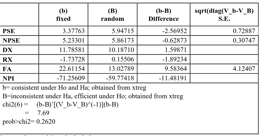
4.3.2 Hausman Test Results
38
hypothesis of correlation between unobservable individual effects and the explanatory variables. Table 4.2 presents the results for the Hausman test.
Table 4. 3: Hausman test results
(b)
fixed
(B) random
(b-B) Difference
sqrt(diag(V_b-V_B) S.E.
PSE 3.37763 5.94715 -2.56952 0.72887
NPSE 5.23301 5.86173 -0.62873 0.30747
DX 11.78581 10.18710 1.59871
RX -1.73728 0.15506 -1.89234
FA 22.61154 13.02789 9.58364 4.12407
NPI -71.25609 -59.77418 -11.48191
b= consistent under Ho and Ha; obtained from xtreg
B=inconsistent under Ha, efficient under Ho; obtained from xtreg chi2(6) = (b-B)’[(V_b-V_B)^(-1)](b-B)
= 7.69 prob>chi2= 0.2620
Source: Computed from the Study Data
The p-value of chi2 for the Hausman test is greater than 0.05, this implies that the null hypothesis is not rejected. Therefore it can be concluded that the most appropriate way of establishing the effects of foreign aid and government expenditure on sectoral GDP growth is a panel model with random effects.
4.4 Effects of Foreign Aid, government expenditure on sectoral GDP growth in Kenya
39 Table 4. 4: Regression results
Dependent Variable: G
Method: Panel EGLS (Cross-section random effects)
Variable Coefficient Std. Error t-Statistic Prob. C 3.934858** 0.421439 9.336718 0.0000
DX -0.095364* 0.049138 -1.940722 0.059
RX -0.434601 1.323411 -0.328395 0.74430
NPI 0.078582** 0.025181 3.120648 0.0033
PSE 0.293068** 0.095886 3.056431 0.0039
NPSE 0.330747** 0.053562 6.175047 0.0000
FA 0.053543 0.289915 0.184686 0.85440
Effects Specification
S.D.
0.297518
Rho 0.1839 Cross-section random
Idiosyncratic random 0.6267 0.8161
Weighted Statistics
R-squared 0.37598 Mean dependent var 0.630043
Adjusted R-squared 0.284661 S.D. dependent var 0.752835 S.E. of regression 0.627708 Sum squared resid 16.15469 F-statistic 4.117179 Durbin-Watson stat 2.263452
Prob(F-statistic) 0.002524
Unweighted Statistics
R-squared 0.337199 Mean dependent var 1.389853 Sum squared resid 17.21567 Durbin-Watson stat 2.123439
*(**) The coefficient is significant at 10% (5%) level of significance Source: Computed from the Study Data
The regression analysis yielded an F-statistic of 4.117 and a corresponding probability value of 0.00252 implying that the independent variables are jointly significant at 5 percent and they jointly influence the dependent variable.
40
acceptable for cross-sectional studies due to the fact that there are other factors apart from the explanatory variables that influence or cause variations in the dependent variable and they vary across the cross-sectional units.
From the results, most of the independent variables’ coefficients are significant, for instance, the coefficient of private (non-public) investments is positive and statistically significant implying that an increase in private investments that is channelled towards agriculture and forestry, education and health sectors lead to an increase in sectoral GDP growth. A one percent increase in non-public or private investments in the above three sectors causes a 0.079 percent increase in sectoral GDP growth holding growth in public sector wage employment, growth in non-public sector wage employment, sectoral foreign aid, sectoral government development expenditure and sectoral recurrent expenditure constant.
The coefficient of the sectoral government development expenditure in agriculture and forestry, health, and education is negative and statistically significant; this means that a one percent increase in sectoral government development expenditure in the above three sectors causes a 0.095 percent increase in sectoral GDP growth holding growth in public sector wage employment, growth in non-public sector wage employment, sectoral private or non-public investment sectoral foreign aid, and sectoral recurrent expenditure constant.
The negative relationship is consistent with other studies such as M’Amanja and Morrissey
(2005) which found that productive/development expenditure has a strong negative impact on economic growth. The negative impact of government development expenditure on sectoral GDP growth according to M’Amanja and Morrissey (2005) could be attributed to the fact that
41
Furthermore, expenditures for public capital investments are sometimes done at an earlier year even before the commencement of the project or later after the completion of the project as opposed to the particular financial year when the expenditure was recorded and at the same time it may take a couple of years before an impact of a capital investment is felt, this may explain the negative relationship.
The coefficient of the government recurrent expenditure was found to be negative and statistically insignificant. The negative relationship is consistent with the findings of other studies such as Maingi (2010) which found that government spending in recurrent activities such as in salaries and wages, debt servicing, operations and maintenance have a growth retarding effect. This can be attributed to wasteful spending on hospitality, travels as well as the bloated public wage bill.