Efficient semiparametric estimation of a partially linear quantile regression model

EFFICIENT SEMIPARAMETRIC

ESTIMATION OF A PARTIALLY

LINEAR QUANTILE

REGRESSION MODEL

S

L

Institute for Fiscal Studies and University College London

This paper is concerned with estimating a conditional quantile function that is assumed to be partially linear+The paper develops a simple estimator of the para-metric component of the conditional quantile+The semiparametric efficiency bound for the parametric component is derived,and two types of efficient estimators are considered+Asymptotic properties of the proposed estimators are established un-der regularity conditions+Some Monte Carlo experiments indicate that the pro-posed estimators perform well in small samples+

1. INTRODUCTION

Many econometrics problems are concerned with estimating a conditional lo-cation function such as conditional mean, conditional median, or conditional

quantile+ Since the seminal work of Koenker and Bassett ~1978!, there have

been many theoretical and applied papers that are related to the estimation of conditional quantiles,including the conditional median as a special case+Most

of these papers are based on a priori assumptions about the functional form of the conditional quantile function₊ The estimation results can be misleading_, however_,if the model is misspecified₊On the other hand_,a fully nonparamet-ric method such as the local polynomial estimator in Chaudhuri~1991a_,1991b! could reduce the possibility of misspecification_,whereas the curse of dimen-sionality occurs as the dimension of independent variables increases₊ Semi-parametric methods that can obtain dimension reduction_,therefore_,are useful because they can avoid the loss of precision due to the curse of dimensional-ity and they make weaker assumptions about the functional form of the regres-sion model+

This paper is a part of my Ph+D+dissertation submitted to the University of Iowa+I am grateful to my adviser,

Joel Horowitz,for his insightful comments,suggestions,guidance,and support+I also thank John Geweke,Gene

Savin,two anonymous referees,the co-editor Oliver Linton,and participants at the 2001 Midwest Econometrics

Group Annual Meeting in Kansas City for many helpful comments and suggestions+Of course,the responsibility

for any errors is mine+Address correspondence to:Sokbae Lee,Department of Economics,University College

London,Gower Street,London WC1E 6BT,U+K+;e-mail:l+simon@ucl+ac+uk+

In particular,this paper develops an estimation method for a partially linear

quantile regression model+The model has the form

Y5qa~X!1Z'ba1Ua, (1)

where Y is a scalar dependent variable_,X is a d_x31 vector of continuous ran-dom variables_,Z is a d_z31 vector of continuous or discrete random variables_, qa~{! is an unknown real-valued function,ba is a dz31 vector of unknown

parameters_,and Uais an unobserved random variable that satisfies Prob~Ua# 0₆X5x_,Z5z!5afor all x and z_,whereaindexes the quantile of interest₊If

a50₊5_,the model reduces to a partially linear median regression model₊ There is a growing literature on estimating semi- and nonparametric quantile regression models+1 For example,see Chaudhuri~1991a,1991b!,Fan,Hu,and

Truong~1994!,and Welsh~1996!for local polynomial quantile regression;see

Chaudhuri,Doksum,and Samarov~1997!,Chen and Khan~2000,2001!,Khan

~2001!, and Khan and Powell ~2001! for semiparametric estimators based on

local polynomial approximations; see Koenker, Ng, and Portnoy ~1994! and

He,Ng,and Portnoy~1998!for smoothing splines;see He and Shi~1994,1996!

for B-spline approximations;see He and Liang~2000!for errors-in-variable

mod-els+Among these papers, three are especially concerned with partially linear

quantile regression models+He and Shi~1996!consider M-type regression splines

using bivariate tensor-product B-splines+He and Liang~2000!develop

estima-tors for linear and partially linear errors-in-variables models+Chen and Khan

~2001! propose an estimation method for a partially linear censored quantile regression+The aforementioned estimators are not asymptotically efficient

un-der the conditional heteroskedasticity of Uain~1!+

The main purpose of this paper is to develop an asymptotically efficient es-timator ofba+2 The paper first develops a simple, two-stage estimator of ba that is an average of nonparametric estimators+ In the first stage, ba is esti-mated locally at each data point by some nonparametric method+These

esti-mates of b_a are averaged in the second stage to obtain the parametric rate of convergence₊This estimator_,which will be called the average quantile regres-sion~AQR!estimator_,is n2102_{-consistent and asymptotically normal}

,but it is

not asymptotically efficient₊The semiparametric efficiency bound forbais cal-culated based on a projection formula_,and then two types of efficient estima-tors of ba are constructed, depending on the assumption about Ua+ If Ua is homoskedastic_,then an optimally weighted version of the AQR estimator can attain the efficiency bound+ When Ua is possibly heteroskedastic, a one-step

asymptotically efficient estimator is used to attain the efficiency bound+

The rest of the paper is organized as follows+Section 2 gives sufficient

con-ditions under whichbaand qa are identified+Section 3 describes the AQR

es-timator of ba+ In Section 4, asymptotic properties of the AQR estimator are

given under a certain set of regularity conditions+In Section 5,the

semipara-metric efficiency bound for ba is derived+ In Section 6, it is shown that the

some Monte Carlo experiments that illustrate the finite sample performance of the proposed estimators+Concluding remarks are given in Section 8+The proofs

of theorems are in the Appendix+

2. IDENTIFICATION OFbaANDqa

Before we consider estimation ofbaand qain~1!,we have to find conditions

under which the partially linear quantile regression model can be identified+

The model is identified ifbaand qaare uniquely determined by the population distribution of~Y,X,Z!+The following result gives sufficient conditions for the

identification of the model+

THEOREM 1₊ Suppose that Prob~Y#qa~X!1Z'ba6X5x,Z5z!5afor all x and z. If

(1) the conditional density of Uais positive at zero for all x and z, and

(2) var~Z6X5x!is nonsingular at every x,

then qaandbaare identified.

The sufficient conditions can be relaxed but are stated in the form used to derive asymptotic properties of the proposed estimators+Condition~1!is

stan-dard but can be relaxed+ For example, Knight ~1998! derives the asymptotic

distributions for linear median regression estimators under a more general as-sumption than condition~1!+See also Smirnov~1952!for limiting distributions

of sample quantiles under general assumptions+Condition~2!excludes a

con-stant variable for Z+Furthermore,it requires that no components of Z be

per-fectly predictable by components of X+A similar but less stringent exclusion

restriction is also needed for partially linear mean regression+For example,it

is assumed in Robinson~1988!that E@var~Z6X!#is positive definite+See

Rob-inson~1988!for detailed discussion+It is assumed throughout the remainder of

this paper thatbaand qaare identified+

3. DESCRIPTION OF THE AVERAGE QUANTILE REGRESSION ESTIMATOR

This section presents the main idea behind the estimation method and de-scribes the AQR estimator of ba+ The estimation procedure involves two

stages:in the first stage,bais estimated locally at each data point;in the

sec-ond stage,these local estimates are averaged to obtain an n2102-consistent

es-timator ofba+

To describe the estimation procedure, we need some notation+ Let $~Yi, Xi,Zi!;1#i#n%be a random sample of~Y,X,Z!in~1!with size n+Let Cn~Xi!

be a cube in Rdx _{centered at X}

iwith side length 2dn,wherednis a sequence of

positive real numbers such thatdnr0+For u5~u1, + + + ,udx!,a dx-dimensional

all dx-dimensional vectors u such that@u##k for some integer k$0 and let

s~Ak!denote the number of elements in Ak+For z[Rdx _{with u}[_A

k,let zu5

)

dx _z

iui+In addition,given X1,X2[ Rdx,define

P_n~c,X1,X2!5

(

c_u

F

dn

G

u

,

where c 5 ~c_u!_u[Ak is a vector of dimension s~Ak!+ Define ra~t! 5 6t6 1

~2a 21!t+ For each Xi, the first-stage estimator bZa~Xi! ofba is defined by

Z

ba~Xi! [bZ,where~c[',bZ'!'is the solution to the following minimization problem:

min

c,b _j5

(

ra$Yj2Pn~c,Xj,Xi!2b'Zj%1~Xj[Cn~Xi!!, (2)

where 1~{!is a standard indicator function+Notice that the preliminary

estima-tor defined here is a leave-one-out estimaestima-tor and a multivariate uniform kernel is used in~2!+

It is important to note that only local data points around Xi are used in~2!+

As a consequence, bZa~Xi! converges in probability to ba at a nonparametric rate+A more efficient estimator forbarequires the use of all data points+

Be-cause bZa~Xi! can be obtained at each data point Xi, the proposed estimation

strategy in this paper is to average allbZa’s to estimateba+This averaging method

ensures that all data points are used and thus leads to a faster rate of convergence+

In the second stage,the AQR estimatorbZaofbais now obtained by

Z

ba5

(

i51 n

tx~Xi!bZa~Xi!

(

i51 n

tx~Xi!

,

wheretx~x!is a trimming function such thattx~x!51~x[X!with a compact

subset Xof Rdx

+The trimming function is introduced to estimate the

param-etersb_awithout being overly influenced by the tail behavior of the distribution of X₊It will turn out in Section 4 that this AQR estimator is n2102_-consistent

forbaand asymptotically normal+

The first-stage estimation procedure is a simplified version of the local poly-nomial estimation procedure developed in Chaudhuri ~1991a_, 1991b! and Chaudhuri et al₊ ~1997!₊ The estimation method considered here is different from that used in Chaudhuri ~1991a, 1991b! and Chaudhuri et al+ ~1997! in

that only a linear term with respect to Z is adopted,no cross products between X and Z are included in ~2!, and local weighting is carried out in terms of

only X,not both X and Z,because the partially linear form of the regression

model is assumed in this paper+A similar type of preliminary estimation

pro-cedure is also considered in Chen and Khan ~2001!+The main advantage of

al-ready well established and can be easily specialized for the purpose of this paper+

We conclude this section by mentioning the numerical algorithm of~2!+

Be-cause the uniform kernel is independent of c and b, the problem ~2! can be

easily shown to have a linear programming representation+From the

perspec-tive of linear quantile regression_,problem~2!can be understood as just weighted quantile regression with weight equal to the uniform kernel₊All computational algorithms developed for linear quantile regression_, therefore_,can be used to solve problem~2! ~see_,e₊g_+,Buchinsky_,1998_,and references therein!₊

4. ASYMPTOTIC PROPERTIES OF THE AVERAGE QUANTILE REGRESSION ESTIMATOR

This section gives regularity conditions under which the AQR estimator ofba is n2102_{-consistent and asymptotically normal}

+ Let 7{7 denote the Euclidean

norm+

Assumption 1+ $~Yi,Xi,Zi!;1 # i # n% is a random sample of ~Y,X,Z!

in~1!+

Let Fa~{6x,z!and fa~{6x,z!,respectively,denote the cumulative distribution

function and the density function of Uaconditional on ~X,Z!5~x,z!+

More-over,let g~x!denote the density function of X and let gxz~x,z!denote the joint

density of X and Z with respect to an appropriate measure+Suppose that Z can

be divided into Z5~Z~c!

,Z~d!!,where Z~c! denote the continuous components

of Z and Z~d! denote the remaining discrete components+Assume that Z~d! has

finitely many mass points₊LetW_xandW_z5W_zc_3W

zd be supports of X and

Z5~Z~c!

,Z~d!!such thatWxandWzcare nonempty convex sets in Rdxand Rdz

c +

Assumption 2+

~a! Fa~06x,z!5afor all~x,z!inWx3Wz,

~b! fa~u6x,z! is bounded away from zero and continuously differentiable with re-spect to u in a neighborhood of zero for all~x,z!inWx3Wz,and

~c! g is positive onWxexcept on the boundary+

Following the nonparametric estimation literature,a function m:RdrR will

be said to have the order of smoothness p on a convex setWin Rd _{with p5}

l1g,where l$ 0 is an integer and 0, g#1,and will be written as m[ Hp~W!,if~i!partial derivatives Dum~x! [ ]@u#m~x!0]x1

u1

+ + +]xd

ud _{exist and are}

continuous for all x[ Wand @u## l and~ii!there exists a constant M . 0 such that

In other words,a function m is l-times continuously differentiable and the lth

derivative is Hölder continuous with exponentg+The order of smoothness,if it

applies to a vector or matrix-valued function,will be understood componentwise+

Assumption 3+ The function qa~{!has the order of smoothness pq. 3dx02

onWx+

Assumption 4+ There exists ag,0, g#1 such that

~a! fa~u6x,z!and gxz~x,z!,as functions of x,belong to Hg~Wx!for all u in a

neigh-borhood of zero and every z inWz,and

~b! g[Hg~Wx!+

Assumption 5+ The distribution of Z has bounded support+

Assumption 6+ dn @ n2k, where k is a positive real number satisfying

10~2pq!,k,10~3dx!+

Assumption 7+ The trimming function tx~x!has compact supportX,where Xhas a nonempty interior andX ,Wx+

Assumption 8+ For all x[Wx,the matrixS~x!is nonsingular,where

S~x!5E

F

S

1 Z'

Z ZZ'

D

*

G

Moreover,S~x!,considered as a function of x,is in Hg~Wx!with someg,0,

g#1+3

It is necessary to make some comments regarding regularity conditions+

Con-dition~a!of Assumption 2 imposes the conditional quantile restriction,and

con-dition~b!is important for identification+Condition~c!ensures that there will

be sufficiently many Xj’s near Xiasymptotically as nr`+This condition with

Assumption 4~b! guarantees that the marginal density of X is bounded away from zero and infinity onX+As done in Chen and Khan~2001!_,it is possible to include discrete random variables for X₊This_,however_,is not explicitly done here for the sake of simplicity₊

Assumption 3 requires that the order of smoothness p_q of qa grow as the dimension of X increases₊4_{Assumptions 4 and 5 are needed to derive a} Bahadur-type expansion similar to that developed in Chaudhuri et al₊~1997!₊5

Assumption 6 restricts the range of the bandwidth₊6 _{As is common in the} semiparametric estimation literature,undersmoothing is required+That is,

As-sumption 6 requires thatdnconverge to zero faster than 10~2pq1dx!, which

is the asymptotically optimal rate for a nonparametric estimator of qa+ This

is not surprising because averaging the first-stage estimators makes the vari-ance of the AQR estimator become smaller than those of the first-stage estima-tors+The left inequality fordnin Assumption 6 is used to make the estimator

remainder terms of the Bahadur-type expansion negligible+ For the trimming

functiontx,aXthat is too small can induce the loss of efficiency,whereas aX

that is too large allows the estimator to be unduly influenced by the tail behav-ior of g~x!+

Finally,Assumption 8 ensures that the variance of the asymptotic

distribu-tion of the estimator is well defined₊7_{In a homoskedastic case where f}

a~06x,z!

is independent of x and z_,Assumption 8 is satisfied if identification conditions in Theorem 1 hold and var~Z₆X5x!is Hölder continuous₊

The next theorem establishes the n2102_{-consistency and asymptotic}

normal-ity of the AQR estimator ofba+Let ez' be the dz3 ~dz11!matrix such that

e_z'5 ~₀

,Idz!,where 0 denotes the dz-dimensional zero vector and Idz an

iden-tity matrix₊

THEOREM 2₊ Suppose that the order of the polynomial in (2) is k5@p_q#. Let bZa denote the AQR estimator of ba. Let Assumptions 1–8 hold. Then as nr_`,

M

V5a~12a!E@$tx*~X!%2ez'S~X!21VS~X!21ez#

with

V5

S

'

Z ZZ'

D

*~_x!5 1~x[X!

Pr~X[X!+

Although the n2102_{-consistency and asymptotic normality of the AQR}

esti-mator are established,the variance V in Theorem 2 is somewhat complicated+

It will be shown in Section 5 that in general this variance is different from the efficient variance bound+The variance V in Theorem 2 can be simplified under

a stronger condition than in Assumption 2+The following corollary restates

Theo-rem 2 under the assumption of homoskedasticity+

COROLLARY 3+ Assume that the conditions in Theorem 2 hold. Further-more, suppose that the conditional density of Ua given x and z, evaluated at zero, is independent of~x,z!, namely, fa~06x,z!5fa~0!for all~x,z!inWx3

Wz. Then as nr`,

M

where

F

V5 a~12a! fa2~0!

E@$t_x*~_X!%2$_E@_ZZ'

The AQR estimator may be compared with other existing estimators in the literature+He and Shi~1996! consider M-type regression splines using

bivari-ate tensor-product B-splines+They establish the asymptotic results under the

assumption that Uais independent of~X,Z!+He and Liang~2000!develop

es-timators for linear and partially linear errors-in-varables models+Their

asymp-totic results are established under a stringent assumption that E~Z₆X5x!50 for all x₊Chen and Khan~2001!propose an estimation method for a partially linear censored quantile regression₊Their estimator uses a two-stage estimation procedure₊In the first stage_,the conditional quantile function is nonparametri-cally estimated by the local polynomial method_,which is also the case for the AQR estimator₊ In the second stage_, they estimate ba by a least-squares-type estimator using differenced values of the estimated conditional quantiles as dependent variables+The implementation of their estimator requires a kind of

tuning parameter that they call a “selection function+” None of the existing

es-timators in the literature are asymptotically efficient under the conditional het-eroskedasticity of Ua+An asymptotically efficient estimator will be constructed

in Section 6+

We end this section by considering estimation of the nonparametric compo-nent qa~{!of the model~1!+Because the parametric componentbacan be esti-mated with an n2102 _rate

, which is faster than the fastest possible rate of

convergence for the nonparametric component,it is possible to estimate qa~{! as asymptotically efficiently as ifba were known+The function qa~{! can be estimated by carrying out a local polynomial quantile regression of Y2Z'bZ

a on X+See Fan and Gijbels~1996,p+202!and Yu and Jones~1998!for

rule-of-thumb bandwidths+

5. THE SEMIPARAMETRIC EFFICIENCY BOUND

In this section,the semiparametric efficiency bound forbawill be derived by adopting the method used in Newey and Powell~1993!+The semiparametric

efficiency bound may be viewed as the supremum of the Cramér-Rao-type bounds for regular parametric submodels+This bound can be calculated

rigor-ously by a projection formula+More specifically,the efficiency bound VB for ba is the inverse of the expectation of the outer product of the efficient score forba,namely,VB5$E@SaSa'#%21,where the efficient score Sais defined by the projection of the score function forbaonto the orthogonal complement of the tangent space in the nonparametric direction+See,for example,Newey~1990!

and Bickel,Klaassen,Ritov,and Wellner~1993!for further discussion+

We consider the following parametric submodel for the nonparametric com-ponent q_a~{!of the regression function_:

q_a,h~{!5q_a~{!1h'_h~{!

,

where h is an arbitrary function of X that satisfies E7h72 , `+As in Newey

paramet-ric submodel for the distribution of~Ua,X,Z!+Instead,we use the existing

re-sults of Newey and Powell ~1990!to derive the efficient scores ~Sba,Sh! for

~ ba',h'!'+Then the efficient score Sa forba will be calculated by finding the projection of Sba onto the orthogonal complement of the tangent space forh+

To begin,it is important to notice that the parametric submodel can be

writ-ten as a linear quantile regression model with parameters~ b_a'

,h'!'+It then

fol-lows from Newey and Powell~1990!that the efficient scores forb_aandhhave the form

S_ba5k~U_a,X,Z!Z and Sh5k~Ua,X,Z!h~X!,

where

k~Ua,X,Z!5

1

a~12a! fa~06X,Z!@a21~Ua#0!#+

By Proposition A+3+5 of Bickel et al+~1993,p+433!,the projection of Sba onto

the tangent space forhcan be calculated by

k~U_a,X,Z!h*~X!5k~Ua,X,Z!$E@k~Ua,X,Z!26X#%21E@Sbak~Ua,X,Z!6X#

5k~U_a,X_,Z!T~X!_,

where

T~X!5 E@fa

2_~0

6X,Z!Z6X# E@f_a2_~0

6X,Z!6X# +

Thus,the efficient score forbais

S_a~Y,X,Z,qa,ba!5Sba2k~Ua,X,Z!h

*~_X!

5 fa~06X,Z!

a~12a! @a21$Y2qa~X!2Z

'b

a#0%# @Z2T~X!#+

This yields the efficiency bound VB

V_B5a~12a!

H

6X,Z!ZZ'#

2E

F

2_~0

6X,Z!Z6X#E@fa2~06X,Z!Z'6X# E@f_a2_~0

6X,Z!6X#

GJ

21

provided that E@S_aS_a'# _{is nonsingular}

+This result implies that the AQR

estima-tor is not efficient in general+If the distribution of Ua is homoskedastic and X and Z are jointly normal,then the variance of the AQR estimator is the same as

the efficiency bound,ignoring the effect of trimming+This does not necessarily

6. EFFICIENT ESTIMATION OFba

This section constructs efficient estimators ofba+When Ua is homoskedastic with respect to Z,more precisely if fa~06x,z!is independent of z,an optimally

weighted AQR estimator will deliver asymptotic efficiency;if Uapermits gen-eral heteroskedasticity,then a one-step estimator will be constructed+

6.1. HomoskedasticUa

In this section_,we will show that the efficiency bound can be attained by con-sidering a weighted version of the AQR estimator₊Because the AQR estimator is just a simple average of the nonparametric estimators_,it is plausible to con-jecture that a weighted average can improve asymptotic efficiency+Indeed,an

efficient estimator ofbacan be obtained by choosing a proper weighting func-tion when Ua is homoskedastic+ To show this, let w~x! be a dz3dz

matrix-valued,weighting function such that E@tx~X!w~X!#is nonsingular and w~x!is

in Hg~Wx!for someg,0, g#1+A weighted AQR estimator bDa can be de-fined as

D

ba5

F

1

n i

(

tx~Xi!w~Xi!

G

F

(

n

tx~Xi!w~Xi!bZa~Xi!

G

It is straightforward to show that when fa~06x,z!5fa~0!for all x and z,

M

where

F

V_w5 a~12a!

f_a2_~0! E@tx~X!w~X!#21E@tx~X!w~X!var~Z6X!21w~X!#

3E@t_x~X!w~X!#21

+

Clearly the optimal choice of the weight function is to set w~x!5var~Z₆X5x!₊ In practical applications_,it is likely that var~Z₆X5x!is unknown_;however_,it can be replaced by its uniformly consistent estimator₊For instance_,we can use the following weighting function_:

[

w~x!5EZ @ZZ'

6X5x#2EZ@Z6X5x#EZ @Z6X5x#',

whereEZ @{6X5x#denotes a kernel estimator of the corresponding expectation+

LetbD_a*_{denote the weighted AQR estimator with weight function w}[~_x!

+In the

THEOREM 4+ Assume that the conditions in Corollary 3 hold. Moreover, suppose that

sup

Xi[X

6w[~Xi!2var~Z6Xi!65op~1!+ Then as nr_`,

M

where

F

V_*5 a~12a!

f_a2_~0! E@tx~X!var~Z6X!#21+

Sufficient conditions for uniform consistency ofw on a compact set can be[ easily obtained using the results of the literature,for example,Bierens ~1983,

1987!and Andrews~1995!+It is easy to see that when fa~06x,z!5fa~0!for all

~x,z!,the varianceVF*is the same as the efficiency bound except for the

exis-tence of the trimming function+The estimator constructed in this paper is not

efficient in a strict sense because it does not use all observations+It is expected

that the loss of efficiency due to the existence of the trimming function could be eliminated by letting the support oftxgrow very slowly as the sample size increases+For example,Robinson~1988!considers the trimming function 1~6fiZ6 .b! ~in his notation!,wherefiZ is a kernel estimator of the probability density

function of Xiand b is a positive constant+The effect of trimming is eliminated

in Robinson~1988!by letting b converge to zero very slowly+In addition,Klein

and Spady~1993!use elaborate trimming procedures to obtain an efficient semi-parametric estimator for binary response models+ Details are not worked out

here,however+

If Ua permits restricted heteroskedasticity, in other words, Ua is homoske-dastic with respect to Z_, it is also possible to construct an efficient estimator via optimal weighting₊More specifically_,if f_a~0₆x_,z!5f_a~0₆x!for all z_,then the asymptotic varianceVF_wfor the weighted AQR estimatorbDahas the follow-ing form_:

F

Vw5a~12a!E@tx~X!w~X!#21E@tx~X!w~X!$fa2~06X!var~Z6X!%21w~X!#

3E@t_x~X!w~X!#21

+

This reveals that the optimal weighting function is w~x!5f_a2_~0

6x!var~Z6X5 x!+The efficiency bound,therefore,can be attained by using a consistent

esti-mator of f_a2_~0

6x!var~Z6X5x!as the weighting function+The conditional

den-sity fa~06x! can be consistently estimated using estimated Ua’s+On the other

hand,if Uapermits general heteroskedasticity,then no weighted AQR

estima-tor can deliver asymptotic efficiency+In the next section,an efficient estimator

6.2. HeteroskedasticUa

In this section, a one-step asymptotically efficient estimator of ba is con-structed by taking one step from the AQR estimator ofba+8 LetbZa denote the AQR estimator defined in Section 3+

If Sa were known except forba,a one-step asymptotically efficient

estima-torbZa*would be obtained by

Z

ba*5bZa1

F

(

i51 n

S_a~Y_i,X_i,Z_i,q_a,bZ_a!S_a~Y_i,X_i,Z_i,q_a,bZ_a!'

G

3

(

i51 n

S_a~Y_i,Xi,Zi,qa,bZa!+

Of course_,this estimator is not feasible because Sacontains unknown popula-tion quantities such as qa~X!,fa~06X,Z!,and T~X!+Moreover,as pointed out

by Newey and Powell~1990!_,the score function is not continuous in param-etersba+As a result of this discontinuity,Newey and Powell~1990!make use

of a sample splitting method for the efficient estimation of a~censored!linear quantile regression model+The sample splitting method adopted in Newey and

Powell ~1990! consists of using each half of the observations to estimate the efficient score for the other half+As a result,the ordering of the data may

mat-ter for the estimation ofba+

Instead of using the technique of Newey and Powell ~1990!, this paper

smooths the score function+Differentiability of the score function enables us to

use standard Taylor series methods to obtain the asymptotic properties of the one-step estimator+The smoothing method requires the introduction of an

ad-ditional tuning parameter,but we feel that this is acceptable because it is very

hard to find any reasonable rule to choose the ordering of the data in practical applications+In addition,it will be shown in Section 7 that the simulation

re-sults are somewhat insensitive to the choice of the tuning parameter+9

Horowitz~1998a!uses a smoothed least-absolute-deviations estimator for a linear median-regression model to obtain asymptotic refinements of boot-strap tests+Following his idea,we replace the indicator function in Sa with a smooth function+Specifically,let J be a bounded,differentiable function

satis-fying J~t!50 if t#21 and J~t!51 if t$1+The function J can be regarded

as the integral of a kernel function+ Let $jn% be a sequence of positive real

numbers that converges to zero₊In addition_,lett~x_,z!51~x[X,z~c!_{[ Z!}

,

where Xand Z are some compact subsets of Rdx _{and R}dzc

, respectively+The

trimming function t~x,z! is introduced for the same reason as before+ For a

given b,a smoothed feasible score functionSZai~b!is then defined as

Z

S_ai~b!5t~X_i,Zi!

Z

f_a~0₆X_i,Z_i!

a~12a!

F

S

Y_i2q[_a~X_i!2Z_i'_b

jn

DG

whereq[a~x!,fZ~06x,z!,andTZ~x!denote consistent estimators of qa~x!,fa~06x,z!,

and T~x!,respectively+Notice that 12J~{0jn!can be arbitrarily close to 1~{#0!

for sufficiently large n+An actual one-step estimator proposed here is

Z

ba*5bZa1

F

(

i51 n

]SZ_ai~bZ_a!0]b

G

21

(

i51 n

Z

S_ai~bZ_a!+ (3)

To complete the description of the one-step efficient estimator, we need to

specify the nonparametric estimators of qa~Xi!,fa~06Xi,Zi!,and T~Xi!+ First

of all,qa~Xi!can be estimated by the first element ofc of[ ~2!+For fa~06x,z!,a

standard kernel density estimator may be used+Observe that fa~06x,z!can be

written as fa~06x,z!5f1~0,x,z!0f2~x,z!,where f1 and f2 are joint densities of ~Ua,X,Z!and~X,Z!,respectively+This suggests that the conditional density of Ua at zero can be estimated consistently by obtaining the ratio of the kernel estimator of f1 to the kernel estimator of f2+More specifically,the kernel

esti-matorfaZ ~06Xi,Zi!is defined as

Z

f_a~0₆X_i,Z_i!5

~nn_1ndx1dz11!21

(

j51 n

t~X_j,Zj!Kuxz

S

Z

U_aj

n1n

, X_j2X_i

n1n

, Z_j2Z_i

n1n

D

~nn_2ndx1dz!21

(

j51 n

t~X_j,Zj!Kxz

S

X_j2X_i

n2n

, Z_j2Z_i

n2n

D

,

whereUZai5Yi2q[a~Xi!2Zi'bZa,Kuxzis a ~dx1dz11!-dimensional kernel

function with a bandwidthn_1n,and K_xzis a~d_x1d_z!-dimensional kernel func-tion with a bandwidthn_2n+Finally_,T~X_i!can be estimated by

Z

T~X_i!5

(

j51 n

t~X_j,Zj!faZ2~06Xj,Zj!ZjKx

S

Xj2Xi

gn

D

(

j51 n

t~Xj,Zj!fZa2~06Xj,Zj!Kx

S

Xj2Xi

gn

D

,

where Kxis a dx-dimensional kernel function with a bandwidthgn+

The following additional regularity conditions are useful to derive the asymp-totic properties of the one-step estimator ofba+

Assumption 9₊ The trimming functiont~x_,z!has compact supportX3Z, whereX3Zhas a nonempty interior andX3Z,Wx3Wzc+

Assumption 10+ The conditional density fa~u6x,z! is continuously twice

differentiable with respect to u in a neighborhood of zero for all ~x,z! in Wx3Wz+

~a! J~{!is bounded,J~v!50 ifv#21,and J~v!51 ifv$1+

~b! J is twice differentiable, J~1!~v! is symmetrical about v50, J~2! is Lipschitz

continuous,and J~i!~v!is bounded for i51,2+

~c! *₂1₁J~1!_~

v!dv51,*21 1

vJ~1!~v!dv50,and*21 1

v2J~1!~v!dv.0+

Assumption 12₊ j_n@n2h_,wherehis a positive real number satisfying 1 4 _ ,

h, 5

18 _

+

Assumption 13+

~a! sup

~Xi,Zi![X3Z

6fZa~06Xi,Zi!2fa~06Xi,Zi!65op~1!+

~b! sup

Xi[X

6TZ~Xi!2T*~Xi!65op~1!,

where

T_*~x!5 E@t~X,Z!fa

2_~0

6X,Z!Z6X5x# E@t~X,Z!fa2~06X,Z!6X5x# +

Assumptions 10–12 are necessary to make smoothing have no effect on the asymptotic distribution of the one-step estimator+Just like the assumption for

[

w in Theorem 4,Assumption 13 is a high-level assumption that requires that

kernel estimators be uniformly consistent on the compact sets+It is easy to

ob-tain sufficient conditions for Assumption 13 using the results of Bierens~1983,

1987!and Andrews~1995!+The main result of this paper is as follows+

THEOREM 5+ Let bZa* denote the one-step estimator defined in (3). Let As-sumptions 1–13 hold. Then as nr`(assuming that V*is well defined),

M

where

V_*5a~12a!

H

2E

F

2_~0

6X,Z!Z6X#E@tfa2~06X,Z!Z'6X# E@tf_a2_~0

6X,Z!6X#

GJ

21

witht5t~X_,Z!.

The variance of Theorem 5 is the same as the efficiency bound except for the effect of the trimming functiont+Just like the case of homoskedastic Ua,

the effect of the trimming function is likely to be eliminated by letting the sup-port oftgrow+

For statistical inference,it is necessary to obtain a consistent estimator of the

simple consistent estimator of V_*that is a by-product of the estimation proce-dure is

Z

V_*5

F

(

]SZ_ai~bZ_a!₀]b

G

21

+

It is shown in the proof of Theorem 5 in the Appendix thatVZ_*converges to V_* in probability+An alternative way to estimate V*is to replace the components

of V_*with its empirical counterparts+A consistent estimator can be given by

Z

V_*5a~12a!

H

(

F

2 EZ @tfa

2_~0

6X,Z!Z6Xi#EZ @tfa2~06X,Z!Z'6Xi#

Z

E@tf_a2_~0

6X,Z!6Xi#

GJ

21

,

where fZ~06x,z! and EZ @{6x# denote consistent nonparametric estimators of fa~06x,z!and E@{6x#+

Adopting the same idea,one can obtain a consistent estimator of the

asymp-totic variance V of the AQR estimator+Specifically,the consistent estimator VZ

has the form

Z

V5a~12a!

F

(

$t[x*~Xi!%2ez'S~Z Xi!21ViS~Z Xi!21ez

G

where

Vi5

S

1 Z_i'

Z_i Z_iZ_i'

D

*~_x!5 1~x[X!

n21

(

1~Xi[X!

,

andS~Z x!is a nonparametric estimator ofS~x!using the estimated fa~06X,Z!+

It is also straightforward to obtain consistent estimators of the variances of the AQR estimator and the weighted AQR estimator when Uais homoskedastic+

7. MONTE CARLO EXPERIMENTS

This section presents the results of a Monte Carlo investigation of the finite sample performance of the proposed estimators in the previous sections+In all

experimentsa50+5 and n5100+Following Robinson ~1988!and Chen and

Khan~2001!,we considered the following model:

Y_i5q~X!1Z'b1s~_X

i,Zi!«i, i51, + + + ,n,

where Xiand Ziwere drawn from a bivariate standard normal distribution with

independent of X and Z+Three different functions for q and two different

func-tions forswere simulated:

q₁~x!511x_, q₂~x!5x14 exp~22x2_!

YY

M

and

s1~x,z!5 3 1

2, s2~x,z!5C exp@0+25~x1z!#,

where C is a constant that was chosen to makes~Xi,Zi!have standard

devia-tion 13 _

+The function q2,which is taken from Härdle~1990,p+122!,has a

bell-shaped hump around zero+ The parameter b was set to be 1+ The trimming

function used in the experiments wastx~x!51~6x6#2!+10

Computing the AQR estimates requires choosing the order of polynomial k and the bandwidthdnin~2!+In the experiments k53+The asymptotic results

of Section 3 only provide the range ofd_nin terms of the asymptotic order₊A higher order asymptotic theory is required to obtain an asymptotically optimal

dn+However, there is a simple, informal selection rule based on the

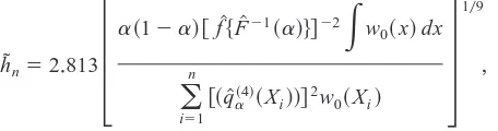
rule-of-thumb bandwidth for the estimation of the nonparametric component qa+LethDn

be the rule-of-thumb bandwidth for the estimation of q when k53_,suggested by Fan and Gijbels~1996_,p₊202!₊Specifically_,hDnis of the form

D

h_n52+813

3

a~12a!@fZ$FZ21_~a!%#22

E

(

i51 n

@~q[_a~4!_~X

i!!#2w0~Xi!

4

,

where w0~{! is a weight function,q[a~x!is obtained from a global polynomial fit, fZ~{! is a kernel density estimate of the residuals of the global polynomial

fit, and FZ21~a! is the ath sample quantile of the residuals+Also, q[a~4!~x! de-notes the fourth derivative ofq[a~x!+The weight function was set to be w0~x!5 1~₆x₆# 2!₊ The global polynomial fit was obtained by carrying out the me-dian regression of Y on the constant term_,X_,X2

, + + + ,X5,and Z+The bandwidth

D

h_n converges at rate n2109

, which is optimal for the estimation of q+

Under-smoothing is required for the estimation of b₊ A simple bandwidth such as

Z

dn5 hDn3 n109 3 n2105 converges at rate n2105 and satisfies Assumption 6

when pq$3+By some preliminary simulations,the averages of ad hoc

band-widths dnZ ranged between 0₊7 and 1₊1 across the designs considered in the experiments+ In the experiments, dn [ $0+5, 0+6, + + + ,1+5%, which includes the

range of the averages ofdnZ +There were 1,000 replications in each experiment+

The computations were carried out in GAUSS with GAUSS pseudo-random number generators+

Figure 1 shows the asymptotic~dashed lines!and empirical~solid lines!root mean squared errors ~RMSEs! of the AQR estimates of b+ The asymptotic

asymptotic variance given in Section 4+For all designs,the empirical RMSEs

are quite close to the asymptotic RMSEs over a wide range of bandwidths in-cluding the range of the average dnZ + It can be seen that the results for q3 are more sensitive to the bandwidth than those for q1and q2,but the results for all

designs are quite insensitive to the bandwidth in the range of the rule of thumb+

The empirical biases of the AQR estimates were also computed and were neg-ligible relative to the empirical standard deviations, so they are not reported

here+

More tuning parameters are required to compute the one-step efficient esti-mates₊The trimming function was set to bet~x_,z!51~₆x₆#2_{, 6}z₆#2!₊ Gauss-ian kernels were used to estimate f_a~0₆X_i,Z_i!₊Bandwidths were n_1n5 n2107

and n_2n 5n2106 _{with respect to standardized designs}

+ For the estimation of T~X_i!_,g_n5s_xn2105

,where sxis the sample standard deviation of X+The

smooth-ing function J is the integral of the quartic kernel such that

J~v!5

5

0 ifv, 21

0+51

15

16

S

3v 3₁1

5 v 5

D

6 v 6#1

1 ifv.1+

The AQR estimates ofband the estimates of q~{! were computed using band-widthdn50+8 Finally,the bandwidth jn has to be chosen,but the asymptotic

theory in Section 5 provides only qualitative restriction for the choice of jn+

The experiments focused on the sensitivity to the choice of jn+In the

experi-ments,jn5$0+1,0+2, + + + ,2+0%+

Figure 2 shows the asymptotic ~dashed lines! and empirical ~solid lines! RMSEs of the one-step estimates ofb+In addition,it also shows the empirical

RMSEs~dotted lines!of the AQR estimates+Asymptotic results given in

previ-ous sections indicate that the AQR estimator is as efficient as the one-step es-timator for homoskedastic designs+Furthermore,the optimally weighted AQR

estimator is basically the same as the AQR estimator because var~Z6X! is a

constant in the experiments+ On the other hand, it can be checked by some

calculation that the asymptotic RMSE of the AQR estimator exceeds that of the one-step estimator by a factor of 1₊4 for heteroskedastic designs₊One notewor-thy result is that the empirical RMSEs of the one-step estimates are somewhat larger than asymptotic counterparts for the heteroskedastic designs₊This is not too surprising because the one-step estimates use several nonparametric esti-mates_, which can be inaccurate for small sample size such as n 5100₊The one-step estimates perform better than the AQR estimates for most of the val-ues of bandwidth jn+It also appears that the results are somewhat insensitive to

the choice of the bandwidth jnas long as jnis not too small+In summary,the

results of Monte Carlo experiments indicate that our proposed estimators work reasonably well in the finite samples+

8. CONCLUSIONS

efficiently estimated+ This paper does not investigate methods for optimally

choosing the tuning parameters that are required to implement the estimation method+Because the asymptotic distributions of the proposed estimators ofba do not depend on bandwidths,a higher order theory is required to choose

mal bandwidths+There is no theoretical work~that we are aware of!regarding

a higher order approximation for semiparametric quantile regression+This is a

topic of future research+Another problem that needs to be studied is how to

conduct a specification test of the regression model+Although partially linear

regression is quite flexible,it still has a possibility of misspecification+It would

be also an interesting problem to test a particular parametric quantile regres-sion model against a partially linear alternative₊

NOTES

1+ For semi- and nonparametric mean regression models,see Härdle~1990!and Horowitz

~1998b!among many others+

2+ See Newey and Powell~1990!and Zhao~2001!for asymptotically efficient estimation of

linear quantile regression models+

3+ The exponentsgin Assumption 4~a!and~b!and Assumption 8 do not have to be same+For

brevity,we assume thatgdenotes the minimum of the threeg’s+

4+ This is common among semiparametric regression estimators+Higher order kernels are

of-ten used when the first-stage estimation is based on kernel-type estimators+Assumption 3 is not

needed to derive the efficiency bound in Section 5,however+

5+ In particular,Assumption 5 is made to exploit Bernstein’s inequality+This assumption can

be satisfied by dropping observations with very large values of Z,if necessary+

6+ Assumption 6 allows for only deterministic bandwidth sequences+It is necessary to use

data-based bandwidths in applications;however,it is beyond the scope of this paper to investigate

the asymptotic properties of the estimator with data-dependent bandwidth sequences+In simple

cases such as nonparametric density and regression estimation,the usual kinds of data-based

band-width selection do not affect the first-order asymptotics of the estimators~see,e+g+,Andrews,1995!+

7+ The condition thatS~x!is nonsingular at every x is stronger than needed to estimateba+

For example,bacan be identified and estimated only using observations for whichS~x!is

nonsin-gular as long as Prob$S~x!is nonsingular%is positive+Assumption 8 is adopted here to minimize

the complexity of the proof+

8+ In fact,any n2102-consistent estimator ofbacan be used as an initial estimator+

9+ Another alternative could be to invoke stochastic equicontinuity arguments in Andrews~1994!+

Unlike the mean regression case,q[ais a step function and therefore is not smooth enough to apply

the existing results in the literature+

10+ If the number of observations that satisfy6Xj2Xi6,dnin~2!is less than 5,which is the

number of regressors in the local cubic fitting,then the estimation procedure will break down+

Hence,those points were additionally excluded in the experiments+

REFERENCES

Andrews,D+W+K+~1994!Empirical process methods in econometrics+In R+F+Engle & D+

McFad-den~eds+!,Handbook of Econometrics,vol+IV,pp+2247–2294+New York:North-Holland+

Andrews,D+W+K+~1995!Nonparametric kernel estimation for semiparametric models+

Economet-ric Theory 11,560–596+

Bickel,P+J+,C+A+J+Klaassen,Y+Ritov,& J+A+Wellner~1993!Efficient and Adaptive Estimation for

Semiparametric Models. Baltimore:Johns Hopkins University Press+

Bierens,H+J+~1983!Uniform consistency of kernel estimators of a regression function under

gen-eralized conditions+Journal of the American Statistical Association 78,699–707+

Bierens,H+J+~1987!Kernel estimators of regression functions+In T+F+Bewley~ed+!,Advances in

Buchinsky,M+~1998! Recent advances in quantile regression models+ Journal of Human

Re-sources 33,88–126+

Chaudhuri,P+~1991a!Global nonparametric estimation of conditional quantile functions and their

derivatives+Journal of Multivariate Analysis 39,246–269+

Chaudhuri,P+~1991b! Nonparametric estimates of regression quantiles and their local Bahadur

representation+Annals of Statistics 19,760–777+

Chaudhuri,P+,K+Doksum,& A+Samarov~1997!On average derivative quantile regression+

An-nals of Statistics 25,715–744+

Chen,S+& S+Khan~2000!Estimating censored regression models in the presence of

nonparamet-ric multiplicative heteroskedasticity+Journal of Econometrics 98,283–316+

Chen,S+& S+Khan~2001!Semiparametric estimation of a partially linear censored regression

model+Econometric Theory 17,567–590+

Fan,J+& I+Gijbels~1996!Local Polynomial Modelling and Its Applications. London:Chapman

and Hall+

Fan,J+,T+-C+Hu,& Y+K+Truong~1994!Robust nonparametric function estimation+Scandinavian

Journal of Statistics 21,433– 446+

Härdle,W+~1990!Applied Nonparametric Regression. New York:Cambridge University Press+

He,X+& H+Liang~2000!Quantile regression estimates for a class of linear and partially linear

errors-in-variables models+Statistica Sinica 10,129–140+

He,X+,P+Ng,& S+Portnoy~1998!Bivariate quantile smoothing splines+Journal of the Royal

Statistical Society, Series B 60,537–550+

He,X+& P+Shi~1994!Convergence rate of B-spline estimators of nonparametric conditional

quan-tile functions+Journal of Nonparametric Statistics 3,299–308+

He,X+& P+Shi~1996!Bivariate tensor-product B-splines in a partly linear model+Journal of

Multivariate Analysis 58,162–181+

Horowitz, J+L+ ~1998a! Bootstrap methods for median regression models+ Econometrica 66,

1327–1351+

Horowitz,J+L+~1998b!Semiparametric Methods in Econometrics. New York:Springer-Verlag+

Khan,S+~2001!Two stage rank estimation of quantile index models+Journal of Econometrics 100,

319–355+

Khan,S+& J+L+Powell~2001!Two-step estimation of semiparametric censored regression models+

Journal of Econometrics 103,73–110+

Klein,R+W+& R+H+Spady~1993!An efficient semiparametric estimator for binary response

mod-els+Econometrica 61,387– 421+

Knight,K+~1998!Limiting distributions for L1regression estimators under general conditions+

An-nals of Statistics 26,755–770+

Koenker,R+& G+Bassett~1978!Regression quantiles+Econometrica 50,43– 61+

Koenker,R+,P+Ng,& S+Portnoy~1994!Quantile smoothing splines Biometrika 81,673– 680+

Newey,W+K+~1990!Semiparametric efficiency bounds+Journal of Applied Econometrics 5,99–135+

Newey,W+K+& J+L+Powell~1990!Efficient estimation of linear and type I censored regression

models under conditional quantile restrictions+Econometric Theory 6,295–317+

Newey,W+K+& J+L+Powell~1993!Efficiency bounds for some semiparametric selection models+

Journal of Econometrics 58,169–184+

Robinson,P+M+~1988!Root-n-consistent semiparametric regression+Econometrica 56,931–954+

Smirnov,N+V+~1952!Limit distributions for the terms of a variational series+American

Mathemat-ical Society Translation,no+67,64 pp+

Welsh,A+H+~1996!Robust estimation of smooth regression and spread functions and their

deriv-atives+Statistica Sinica 6,347–366+

Yu,K+& M+C+Jones~1998!Local linear quantile regression+Journal of the American Statistical

Association 93,228–237+

Zhao,Q+~2001!Asymptotically efficient median regression in the presence of heteroskedasticity

APPENDIX

A.1. The Proofs of Theorems+This part of the Appendix provides the proofs of

theo-rems+The proofs of Corollary 3 and Theorem 4 are omitted because they are straight-forward modifications of the proof of Theorem 2+The stochastic order symbols such as op~1! or Op~1! will be understood componentwise+ In addition, 6{6 is also considered componentwise+Let Uai5Yi2qa~Xi!2Zi'ba+

Proof of Theorem 1. Let Fy~{6x,z! denote the conditional distribution of Y given

X5x and Z5z+Then we have Fy21~a6x,z!5qa~x!1z'b

a+Notice that Fy21is unique

given x and z by condition~1!+Rewrite this as

~1 z'!

S

qa~x!

ba

D

F_y21_~a

6x,z!+

Premultiplying both sides by~1 z'!'

,we have

S

z zz'

DS

qa~x!

ba

D

S

Fy21~a6x,z!

zFy21~a6x,z!

D

for all x and z+Taking expectations on both sides given x,we have

S

E@Z6X5x# E@ZZ'6X5x#

DS

qa~x!

ba

D

S

E@Fy21~a6X,Z!6X5x#

E@ZFy21~a6X,Z!6X5x#

D

+

Notice that qa~x!is just a point given x+If condition~2!is satisfied,then the matrix on the left-hand side is invertible+This implies that qa~x!andbaare uniquely determined+ Because the choice of x is arbitrary,this completes the proof+

n

Proof of Theorem 2. Let ntx5

(

n

tx~Xi!+Write

Z

ba2ba5

1

n_t

x

(

i51

n

tx~Xi!$bZa~Xi!2ba%

5 1

n Pr~X[X!i

(

n

tx~Xi!$bZa~Xi!2ba%1Rtx,n

[Tn1Rtx,n+

First notice that Rtx,nresults from the replacement of ntxwith n Pr~X[X!+It is easy to

see that Rtx,n5op~n2102!because Pr~X[X!is the expectation oftx~X!+

we need additional notation+Let b~dn,Xj2Xi,Zj!denote the~s~Ak!1dz!-dimensional

vector

b~dn,Xj2Xi,Zj!5~$dn2@u#~Xj2Xi!u,@u##k%',Zj'!' (A.1)

and let Gn~Xi!denote the~s~Ak!1dz!3~s~Ak!1dz!matrix

Gn~Xi!5

E

@21,1#dx

E

f_a~06Xi1dnt,z!b~1,t,z!b~1,t,z!'dPZ~z6Xi1dnt!

3gdn~t,Xi!dt, (A.2)

where

gdn~t,Xi!5

g~Xi1dnt!

E

g~Xi1dnt!dt

+

Also,PZ~z6x!denotes a probability measure with respect to Z given X5x+Let e' de-note the dz3~s~Ak!1 dz! matrix such that e' 5~0,Idz!, where 0 denotes the dz3

s~Ak!-dimensional zero matrix and Idzan identity matrix+In addition,let Nn~Xi!denote

the number of all j ’s satisfying6Xj2Xi6#dnfor jÞi,j51, + + + ,n,and let qa*~Xj,Xi!

be the k-order Taylor polynomial defined in~A+10!,which follows+ It follows from Lemma 1 in the second section of this Appendix that

Z

ba~Xi!2ba5e'$Nn~Xi!Gn~Xi!%21

5

(

j51,jÞi n

b~dn,Xj2Xi,Zj!@a21$Yj#qa*~Xj,Xi!1Zj'ba%#

31$6Xj2Xi6#dn%1Rn~Xi!, where

max

Xi[X

6Rn~Xi!65o~n2102! almost surely as nr`,

provided that 10~2pq1d!,k,10~3dx!+It is worth noting that b~dn,Xj2Xi,Zj!and

Gnare different from those of Chaudhuri et al+~1997!because a partially linear regres-sion model is considered here+

Now substituting the Bahadur-type expansion ofbZa~Xi!2bainto Tnand following

arguments similar to those in the proof of Theorem 2+1 of Chaudhuri et al+~1997! ~in particular,we require 10~2pq!,k,10~3dx!!,we have

Tn5Un1op~n2102!,

where Unis a U-statistic with the kernel dependent on n:

Un5

(

1#i,j#n

with zi5 ~Yi,Xi,Zi!, jn~zi,zj! 5hn~zi,zj! 1 hn~zj,zi!, pn~X! 5dndx*@21,1#dxg~X1

dnt!dt,and

hn~zi,zj!5

1

ntx

*~_X

i!e'$npn~Xi!Gn~Xi!%21b~dn,Xj2Xi,Zj!$a21~Uaj#0!%

31$6Xj2Xi6#dn%+

Define Pnto be the projection of Un,so that

Pn5~n21!

(

i51

n

mn~zi!,

where

mn~zi!5E@jn~zi,zj!6zi#

5 1

n2$a21~Uai#0!%

3E@tx*~Xj!e'$pn~Xj!Gn~Xj!%21b~dn,Xi2Xj,Zi!1$6Xi2Xj6#dn%6Xi,Zi#+

As in the proof of Theorem 2+1 of Chaudhuri et al+~1997!,an application of the stan-dard Hoeffding decomposition of Unyields

E~Un2Pn!25

n~n21!

2 ~Ejn

2_~z

1,z2!22Emn2~z1!!

#n~n21!

2 Ejn

2_~z 1,z2!

#2n~n21!Ehn2~z1,z2!+

Using the facts that~a! in view of Assumption 8, 7Gn21~Xi!7is uniformly bounded for Xi[Xas nr`,~b!pn~Xi!5dndx*@21,1#dxf_a~X_i1d_nt!dt_,and~c!each component of

b~dn,X22X1,Z2!1$6X22X16#dn% is bounded,we have

Ehn2~z1,z2!5O~10n4dn2dx!+

This implies that

E~Un2Pn!25O

S

1

n2_d

n2dx

D

and,hence,using Assumption 6,

Un5Pn1op~n2102!+

The next step is to evaluate the limit of the projection Pn+We will show subsequently that

where

E

Pn5

n21

n2

(

i51

n

$a21~Uai#0!%tx*~Xi!n~Xi,Zi!

with

n~x,z!5ez'E

F

S

Z ZZ'

D

*

G

21

S

z

D

Conditioning on~Xi,Zi!,we have

E~Pn2PEn!25

~n21!2_a~12a!

n3 E$E@tx*~Xj!e'$pn~Xj!Gn~Xj!%21b~dn,Xi2Xj,Zi!

31$6Xi2Xj6#dn%6Xi,Zi#2tx*~Xi!n~Xi,Zi!%2+

(A.4)

As in Lemma 4+2~b!of Chaudhuri et al+~1997!,it can be shown that

dndx$pn~Xj!Gn~Xj!%21

5

H

E

@21,1#dx

E@b~1,t,Z!b~1,t,Z!'fa~06X,Z!6X5Xj#dt

J

21

1OL2~d_ng!_,

where OL2~{!denotes a remainder term that is bounded in the L₂norm₊By a change of

variables,the inner expectation in~A+4!becomes

E

tx*~Xi2dnu!e'

H

E

@21,1#dx

E@b~1,t,Z!b~1,t,Z!'fa~06X,Z!6X5Xi2dnu#dt

J

21

3b~1,u,Zi!du1OL2~dng!+

Using this and a Taylor series expansion, we can show that the outer expectation in

~A+4!converges to zero,which proves~A+3!+By Chebyshev inequality,~A+3!implies

Pn5PEn1op~n2102!+

Therefore,

M

1

M

(

n

$a21~Uai#0!%tx*~Xi!n~Xi,Zi!1op~1!,

from which the desired result follows immediately using the multivariate central theorem+

n

Proof of Theorem 5. Let I*5V*

21

+Write

M

M

F

(

i51

n

]SZai~bZa!0]b

G

n2102

(

i51

n

Z

Let

Sai~b!5t~Xi,Zi!

fa~06Xi,Zi!

a~12a! @a21$Yi2qa~Xi!2Zi

'_b#₀%# @_Z2_T *~X!#+

It will be shown subsequently that

2n21

(

i51

n

]SZai~bZa!0]b5I*1op~1!, and (A.5)

n2102

(

i51

n

Z

Sai~bZa!5n2102

(

i51

n

Sai~ ba!2I*

M

It then follows that

M

21_n2102

(

i51

n

S_ai~ ba!1op~1!,

which gives the desired result immediately+

As in Lemma 4+3~a!of Chaudhuri et al+~1997!,it can be shown that

sup

Xi[X

6q[~Xi!2qa~Xi!65op~n2103!+ (A.7)

In fact,we require that 10~2pq1dx!,k,10~3dx!in view of Lemma 1~in particular, see step 3 in the proof!+Furthermore,by similar arguments as in the proof of Theo-rem 2,it can be proved that

n21

(

i51

n

tx~Xi!@q[~Xi!2qa~Xi!#5Op~n2102!+ (A.8) Letti5t~Xi,Zi!,fi5fa~06Xi,Zi!,andfiZ 5faZ ~06Xi,Zi!for shorthand notation+To show~A+5!,note that

2n21

(

i51

n

]SZai~bZa!0]b5 1

njni

(

n _t ifZi

a~12a!J

~1!

S

jn

D

@Zi2TZ~Xi!#Zi'

5 1

njni

(

n _t ifi

a~12a!J

~1!

S

jn

D

@Zi2T*~Xi!#Zi'1op~1!

5 1

nj_ni

(

n _t ifi

a~12a!J

~1!

S

j_n

D

5I*1op~1!,