Quantization in Continuous-Source Zero Secrecy Leakage Helper Data Schemes

Information Leakage of Continuous-Source Zero Secrecy Leakage

Helper Data Schemes

Joep de Groot, Boris ˇ

Skori´c, Niels de Vreede, Jean-Paul Linnartz

Abstract

A Helper Data Scheme (HDS) is a cryptographic primitive that extracts a high-entropy noise-free string from noisy data. Helper Data Schemes are used for preserving privacy in biometric databases and for Physical Unclonable Functions. HDSs are known for the guided quantization of continuous-valued biometrics as well as for repairing errors in discrete-continuous-valued (digitized) extracted values. We refine the theory of Helper Data Schemes with the Zero Leakage (ZL) property, i.e., the mutual information between the helper data and the extracted secret is zero. We focus on quantization and prove that ZL necessitates particular properties of the helper data generating function: (i) the existence of “sibling points”, enrollment values that lead to the same helper data but different secrets; (ii) quantile helper data.

We present an optimal reconstruction algorithm for our ZL scheme, that not only minimizes the reconstruction error rate but also yields a very efficient implementation of the verification. We compare the error rate to schemes that do not have the ZL property.

Keywords: Biometrics, fuzzy extractor, helper data, privacy, secrecy leakage, secure sketch.

1

Introduction

1.1

Biometric Authentication

Biometrics have become a popular solution for authentication or identification, mainly because of its convenience. Biometric features cannot be forgotten (like a password) or lost (like a token). Nowadays identity documents such as passports nearly always include biometric features extracted from fingerprints, faces or irises. Governments are storing biometric data for fighting crime and some laptops and smart phones use biometrics-based user authentication.

In general biometrics are not strictly secret. Fingerprints can be found on many objects. It is hard to prevent one’s face or irises from being photographed. Nonetheless, one does not want to store biometric features in an unprotected database since this will make it easier for an adversary to misuse them.

Storage of the features introduces both security and privacy risks for the user. Security risks include the production of fake biometrics from the features, e.g., rubber fingers [14, 18]. These fake biometrics can be used to obtain unauthorized access to information or services or to leave fake evidence at crime scenes.

We mention two privacy risks. (i) Some biometrics are known to reveal diseases and disorders of the user. (ii) Unprotected storage allows for cross-matching between databases.

The security and privacy problems cannot be solved by simply encrypting the database. An important

part of the standard attack model isinsider attacks, i.e., attacks by people who are authorized to access

the database. They possess the decryption keys; hence database encryption does not stop them. All in all, the situation is very similar to the problem of password storage. The standard solution is

to storehashedpasswords. Cryptographic hash functions are one-way functions, i.e., inverting them is

computationally infeasible. An attacker who gets hold of a hashed password cannot deduce the password from it.

w1 r

z x1

y1

Gen 2

Rep 2

h

h ₌? Accept_Y/N

Enrollment Verification

x

y

c

ˆ c s1

ˆ k

h(ckz)

h(ˆckz) xM

transform

transform yM

wM

sM

ˆ s1

ˆ sM

k Gen 1

Rep 1

Stage 1 HDS Stage 2 HDS

concat-enate

concat-enate

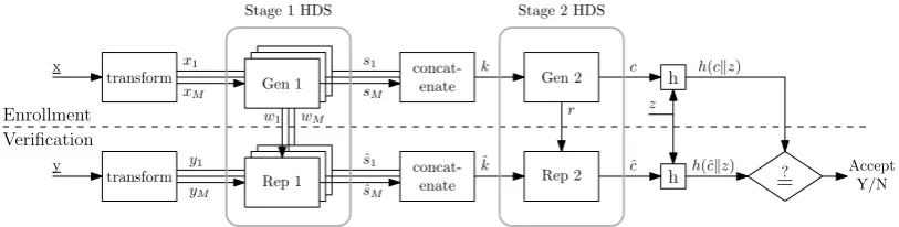
Figure 1: Common steps in a privacy-preserving biometric verification scheme.

1.2

Two Stage Approach

Fig. 1 describes a commonly adopted two-stage approach, as for instance presented in [17, Chap. 16].

A Helper Data Scheme (HDS) consists of two algorithms,GenandRep. TheGentakes a noisy value

as input and generates a secret and so-called helper data. TheRepalgorithm has two inputs: the helper

data and a noisy value correlated with the first one. It outputs an estimator for the secret made byGen.

The stage 1 HDS in Fig. 1 processes the signals during an optimized bit extraction [3, 6, 12]. Helper data is applied in the ‘analog’ domain, i.e., before ‘bit-mapping’: per dimension, the orthogonalized

biometric xis biased towards the center of a quantization interval, e.g., by adding a helper data value

w.

The stage 2 HDS employs digital error correction methods with discrete helper data, for instance the

helper data is the XOR of secretkwith a random codeword from an error-correcting code [9].

Such a two-stage approach is also common practice in communication systems that suffer from un-reliable (wireless) channels: the signal conditioning prior to the bit mapping involves optimization of signal constellations and multidimensional transforms. In fact, the discrete mathematical operations, such as error correction decoding, are known to be particularly effective for sufficiently error-free signals. According to the asymptotic Elias bound [13, Chap. 17], at bit error probabilities above 10% one cannot achieve code rates better than 0.5. Similarly, in biometric authentication, optimization of the first stage appears essential to achieve adequate system performance.

In a preparation phase preceding all enrollments, the population’s biometrics are studied and a transform is derived (using well known techniques such as PCA/LDA [21]) that splits the biometric

vector x into scalar components (xi)Mi=1. We will refer to these componentsxias features. The transform

ensures that they are mutually independent, or nearly so.

At enrollment, a person’s biometric x is obtained. The transform is applied, yielding features (xi)Mi=1.

The Genalgorithm of the first-stage HDS is applied to each feature independently. This gives

contin-uous helper data (wi)Mi=1 and short secret stringss1, . . . , sM which may or may not have equal length,

depending on the signal-to-noise ratio of the features and subsequent choice of allocated number of bits.

All these secrets are combined into one high-entropy secret k, e.g., by concatenating them after

Gray-coding. Biometric features have a within-class Probability Density Function (PDF) that, with multiple

dimensions, will lead to some errors in the reproduced secret ˆk; hence a second stage of error correction

is done with another HDS. The output of the second-stageGenalgorithm is discrete helper datar and

a practically noiseless string c. The hash h(ckz) is stored in the enrollment database, along with the

helper data (wi)Mi=1 andr. Herez is salt: a random string to prevent easy cross-matching.

In the authentication phase, a fresh biometric measurement y is obtained and split into components

(yi)Mi=1. For each i independently, the estimator ˆsi is computed from yi andwi. The ˆsi are combined

into an estimator ˆk, which is then input into the 2nd-stage HDS reconstruction together with r. The

result is an estimator ˆc. Finallyh(ˆc_kz) is compared with the stored hashh(c_kz).

1.3

Secret Extraction

Special algorithms have been developed for HDSs [3,6,7,12]: Fuzzy Extractors (FE) and Secure Sketches (SS). The FE and SS are special cases of the general concept and in our case can apply to both the stage 1 and 2 HDS. The algorithms have different requirements,

ˆ Fuzzy Extractor

00 01 11 10

verification samplex

p ro b a b ilit y d en sit y tization background PDF genuine user PDF quantization boundary

-3 -2 -1 0 1 2 3 0 0.2 0.4 0.6 0.8 1 1.2 1.4 1.6 1.8 2

(a)Fixed equiprobable quantization

q

1 0 1 0 1 0 1 0

verification samplex

p ro b a b ilit y d en sit y background PDF genuine user PDF quantization boundary

-3 -2 -1 0 1 2 3 0 0.2 0.4 0.6 0.8 1 1.2 1.4 1.6 1.8 2

(b)Quantization Index Modulation

00 01 11 10 00

verification samplex

p ro b a b ilit y d en sit y / lik elih o o d ra tio background PDF genuine user PDF likelihood ratio quantization boundary

-3 -2 -1 0 1 2 3 0 1 2 3 4 5 6

(c)Multi-bits based on likelihood ratio [3]

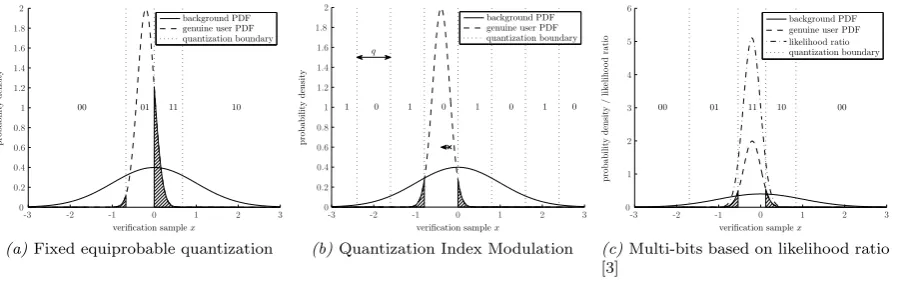
Figure 2: Examples (of adaptation to) the genuine user PDF during verification. Fixed equiprobable quantization does not translate the PDF, quantization index modulation centers the PDF on a quantiza-tion interval and the Multi-bits likelihood ratio based scheme of Chen et al. [3] uses the likelihood ratio to adjust the quantization regions.

ˆ Secure Sketch

s given w must have high entropy, but does not have to be uniform. Typicallys is equal to (a

discretized version of)x.

The FE is typically used for the extraction of cryptographic keys from noisy sources such as Physical Unclonable Functions (PUFs) [8, 15, 20]. Some fixed quantization schemes support the use of a fuzzy

extractor, provided that the quantization intervals can be chosen such that each secretsis equiprobable,

as in [16].

The SS is very well suited to the biometrics scenario described above.

1.4

Security and Privacy Preservation

In the HDS context, the main privacy question is how much information, andwhichinformation, about

the biometric x is leaked by the helper data. Ideally, the helper data would contain just enough

in-formation to enable the error correction. Roughly speaking this means that the vector w = (wi)Mi=1

consists of the noisy ‘least significant bits’ ofx, which typically do not reveal sensitive information since

they are noisy anyway. In order to make this kind of intuitive statement more precise, one studies the information-theoretic properties of HDSs. In the system as sketched in Fig. 1 the mutual information

I(C; W, R) is of particular interest: it measures the leakage about the string c caused by the fact that

the attacker observes w andr. By properly separating the ‘most significant digits’ ofxfrom the ‘least

significant digits’, it is possible to achieve I(C; W, R) = 0. We call this Zero Secrecy Leakage or, more

compactly, Zero Leakage (ZL). HDSs with the ZL property are very interesting for quantifying privacy

guarantees: if a privacy-sensitive piece of a biometric is fully contained inc, and not in (w, r), then a ZL

HDS based database revealsabsolutely nothingabout that piece.

If in a concatenation of multiple stages of the HDS, each stage has ZL, this is a sufficient condition

that also I(C;W, R) = 0. Therefore we will focus in particular on schemes whose first stage has the ZL

property I(Si, Wi) = 0. Yet, I(Si, Wi) = 0 is not a necessary condition for I(C;W, R) = 0. In fact, a

counter example is that one can simply eliminate all dimensions for which I(Si, Wi)>0 in the second

stage of the HDS to achieve I(C;W, R) = 0. However, this would reduce the entropy in the extracted

secret C and is therefore not attractive.

1.5

Biometric Quantization

Biometric quantization, or at least a translation from finely quantized features to a coarse bit-mapping, takes place in the first-stage HDS of a common biometric verification scheme as depicted in Fig. 1. Some concepts, which we will briefly discuss in this section, have already been developed for this stage.

1.5.1 Fixed Quantization (FQ)

The simplest form of quantization applies a uniform, fixed quantization grid during both enrollment and

verification. An example forN = 4 quantization regions during verification is depicted in Fig. 2a. As can

be seen in the figure an unfavorably located genuine user PDF can cause a high reconstruction error (the hatched areas). The inherently large error probability can be mitigated by ‘reliable component’ selection [16]. Only dimensions that are likely to repeatedly deliver realizations within the same quantization interval are selected during the enrollment. Hence the verification relies on features which for that biometric prover have most of their PDF mass within the same interval. The selection of dimensions is also conveyed to the verification phase as user-dependent helper data.

In such a scheme the verification capacity is not optimally used: features that are unfavorably lo-cated w.r.t. the quantization grid, but nonetheless carry information, are eliminated. Revealing which dimensions are not near quantization boundaries may leak information about the actual result of the quantization. The outer intervals, as depicted in Fig. 2a, are wider and therefore are more likely to produce ‘reliable components’ than the inner intervals, which can cause leakage when no precautions are taken [10].

Implicitly, the fixed quantization case also covers systems that only implement a stage 2 HDS. Po-tentially such systems can be further improved by adaptive quantization, as illustrated below.

1.5.2 Quantization Index Modulation (QIM)

This method borrows principles from digital watermarking [2] and writing on dirty paper [4]. QIM uses

alternating quantization intervals labeled with ‘0’ and ‘1’ as the values for the secret s. Based on the

enrollment sample, an offsetw is calculated which is added to bias the verification sample towards the

center of a quantization interval as depicted in Fig. 2b. If the bias is always exactly to the center of a

quantization interval of sizeq, the probability of an error for a Gaussian sample pair is

pQIM

e ≈erfc

_q

2√2σ

(1)

In fact, for a fixed quantization, i.e., without the helper data bias towards the center of quantization intervals, if the biometrics were locally approximately uniform, i.e., if the biometric lies at a random position in the quantization interval, the error probability is much larger, namely [1, Ch. 7]

pFQe =

1 q

Z q/2

−q/2

erfc

_q/2

−x

2√2σ

dx _→

r

2 π

σ

q (2)

forqsufficiently larger than the within-class standard deviation σ. Numerical evaluation of (1) and (2)

shows that to ensure an error rate less than 10%, biased quantization, such as QIM can tolerateq_≈3.3σ,

while fixed quantization would require q >8σ. This implies that in practical systems, the omission of

stage 1 HDS, but relying on stage 2 HDS, jeopardizes extraction of more than one bit per dimension. Moreover, it illustrates the substantial enhancement that helper-data guided quantization can bring in a stage 1 HDS and has been a motivation for this work.

QIM allows a choice in quantization step sizes to make a trade-off between verification performance and leakage [12]. The alternating bit-mapping was adopted to reduce leakage but sacrifices entropy extraction. However, our results show quantization schemes that outperform this.

1.5.3 Likelihood based Quantization (LQ)

Chen et al. [3] improves the reconstruction rate by exploiting the likelihood ratio to set the quantiza-tion scheme. Based on some enrollment samples, the genuine user’s PDF is estimated, which is used to determine a likelihood ratio. It is assumed that the background PDF is known and equal during

enroll-ment and verification. The scheme allocates quantization regions for|S| =N different secret values as

depicted in Fig. 2c. The first two quantization boundaries for the verification phase are then chosen such

that they are at an equal likelihood ratio and at the same time enclose a probability mass of 1/N on the

background distribution. Subsequent quantization intervals are chosen contiguous to the first and enclose

again a 1/Nprobability mass. Finally the probability mass in the tails of the distribution is added up as

a wrap-around interval, which also holds a probability mass of 1/N. Since the quantization boundaries

Likelihood based quantization does not provide an equiprobable secretsand therefore does not qualify

as a fuzzy extractor. Moreover,I(T;S)6= 0 which implies there is some secrecy leakage from the public

verification thresholdtto the enrolled secrets.

The work in this paper does not a priori choose a quantization for enrollment and verification, but imposes the requirement of zero secrecy leakage and a low reconstruction error rate to come to an optimal quantization scheme.

1.6

Contributions and Organization of This Paper

In this paper we zoom in on the first-stage HDS and focus on the ZL property in particular. Our aim is

to minimize reconstruction errors in ZL HDSs that have scalar input x∈R. We treat the helper data

as being real-valued,w∈R, though of coursewis in practice stored as a finite-precision value.

ˆ We show that the ZL constraint for continuous helper data necessitates the existence of ‘Sibling

Points’, points xthat correspond to differentsbut give rise to the same helper dataw.

ˆ We prove that the ZL constraint forx∈Rimplies ‘quantile’ helper data. This holds for uniformly

distributed s as well as for non-uniform s. Thus, we identify a simple quantile construction as

being the generic ZL scheme for all HDS types, including the FE and SS as special cases. It turns out that the continuum limit of a FE scheme of Verbitskiy at al. [19] precisely corresponds to our quantile HDS.

ˆ We derive a reconstruction algorithm for the quantile ZL FE that minimizes the reconstruction

errors. It amounts to using a set of optimized threshold values, and is very suitable for low-footprint implementation.

ˆ We analyze, in an all-Gaussian example, the performance (in terms of reconstruction error rate) of

our ZL FE combined with the optimal reconstruction algorithm. We compare this scheme to fixed quantization and a likelihood-based classifier. It turns out that our error rate is better than that of fixed quantization, and not much worse than that of the likelihood-based classifier.

The organization of this paper is as follows. The sibling points and the quantile helper data are treated in Section 3. Section 4 discusses the optimal reconstruction thresholds. The performance analysis in the Gaussian model is presented in Section 5.

2

Preliminaries

2.1

Quantization

Random variables are denoted with capital letters and their realizations in lowercase. Sets are written in calligraphic font. We zoom in on the one-dimensional first-stage HDS in Fig. 1. For brevity of notation

the indexi_{∈ {}1, . . . , M_}onxi, wi,si,yi and ˆsi will be omitted.

The Probability Density Function (PDF) or Probability Mass Function (PMF) of a random variableA

is denoted asfA, and the Cumulative Distribution Function (CDF) asFA. The helper data is considered

continuous,W _{∈ W ⊂}R. The secretSis an integer in the rangeS ={0, . . . , N−1}, whereN depends on

the signal-to-noise ratio of the biometric feature. The helper data is computed fromX using a function

g, i.e.,W =g(X). Similarly we define a quantization function Qsuch that S=Q(X). The enrollment

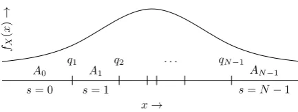
part of the HDS is given by the pairQ, g. We define quantization regions as follows,

As={x∈R:Q(x) =s}. (3)

The quantization regions are non-overlapping and cover the complete feature space, hence form a parti-tioning:

As∩At=∅ fors6=t;

[

s∈S

As=R. (4)

We consider only quantization regions that are contiguous, i.e., for all s it holds that As is a simple

interval. In Section 4.2 we will see that many other choices may work equally well, but not better;

our preference for contiguous As regions is tantamount to choosing the simplest element Q out of a

A0 A1 AN−1

q1 q2 qN−1

s= 0 s= 1 s=N−1

. . .

x→

fX

(

x

)

→

Figure 3: Quantization regions As and boundariesqs. The locations of the quantization boundaries are

based on the distribution of x, such that secret soccurs with probabilityps.

quantization boundaries qs = infAs. Without loss of generality we choose Q to be a monotonically

increasing function. This gives supAs=qs+1. An overview of the quantization regions and boundaries

is depicted in Fig 3.

In a generic HDS the probabilitiesP[S =s] can be different for eachs. We will use shorthand notation

P[S=s] =ps>0. (5)

The quantization boundaries are given by

qs=FX−1 s−1

X

t=0

pt

!

, (6)

whereF_X−1 is the inverse CDF. For a Fuzzy Extractor one requiresps= 1/N for alls, in which case (6)

simplifies to

qFE

s =FX−1

s

N

. (7)

2.2

Noise Model

We assume the verification sampley to be related to the enrollment samplexas follows

Y =λX+R, (8)

in whichλ_∈[0,1] is the attenuation parameter andR independent additive noise. Hence

σ2Y =λ2σ2X+σ2R. (9)

In this equationσ2

X, σY2 and σR2 denote the variance of the enrollment sample, verification sample and

noise respectively. One often uses the correlationρ_∈[₋1,1], defined as

ρ=E[XY]−E[X]E[Y] σXσY

. (10)

By using this equation we can derive an expression forλ

λ2= ρ

2

1₋ρ2

σR2

σ2

X

. (11)

and for the signal-to-noise ratio (SNR)

SNR = λ

2_σ2

X

σ2

R

= ρ

2

1₋ρ2 (12)

In this model we can identify two limiting situations

1. Perfect enrollment

The enrollment can be conditioned such that noise has negligible influence. However, the verifica-tion will be subject to noise. In this situaverifica-tion we get

x

_−→

w

−

→

N=4

s

= 0

1

2

3

x

x

x

x

p0

= 0

.

4

p1

= 0

.

2

p2

= 0

.

3

p3

= 0

.

1

-2

-1

q

0

q

1

q

2

0

0.2

0.4

0.6

0.8

1

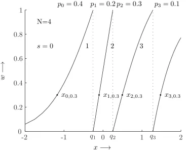
Figure 4: Example of helper data generating function g for a standard Gaussian distribution, i.e. x_∼ N(0,1), andN= 4. Sibling pointsxsw are given fors∈ {0, . . . ,3} andw= 0.3.

2. Identical conditions

The enrollment and verification recordings are identical in terms of noise. In this situation we get

σ2

Y =σ2X ⇐⇒

λ2_=ρ2

σ2

R= (1−ρ2)σ2X

. (14)

Definition 2.1:The noise is calledsymmetric fading noise if for allx, y1, y2 it holds that

|y1−λx|>|y2−λx| =⇒ fY|X(y1|x)< fY|X(y2|x). (15)

An example of a distribution that satisfies the requirements, i.e., symmetric and fading, and has

correlationρis a jointly Gaussian biometric, given by

X ∼ N(0,1), (Y|X=x)∼ N(ρx,1−ρ2). (16)

This distribution corresponds to the “Identical conditions” situation and yields the quantization pattern as depicted in Fig. 6c.

3

Zero Leakage Helper Data

First we will derive properties for the helper data generating functiongthat are required for reproduction.

These properties will be taken into account when deriving the requirements for zero leakage in the second part of this analysis.

3.1

Requirements for Reproduction

During a verification the verifier will reconstruct xs samples based on the public helper data w and

compare the measured verification sampleyto them. Based on our assumptions of the noise, as explained

in Section 2.2, the originator xs scaled by λ, which is the closest to y will be selected to produce the

estimate of the secret ˆs. Hence, the minimum distance between thesexsoriginators has to be maximized,

F

(

x

)

−→

w

−

→

N=4

s

= 0

1

2

3

p0

= 0

.

4

p1

= 0

.

2

p2

= 0

.

3

p3

= 0

.

1

0

_F

₍

_q

₎

_F

₍

_q

₎

_F

₍

_q

_{) 1}

0

0.2

0.4

0.6

0.8

1

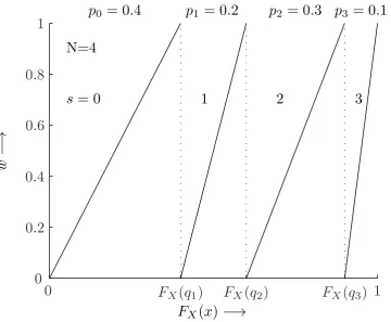
Figure 5: Example of helper data generating function g for N = 4 on quantile x, i.e. FX(x). Sibling

pointsusw = (s+w)/N are given for s∈ {0, . . . ,3} andw= 0.3.

Lemma 3.1:Let _{W ⊂} Rbe the set of possible helper data values. Let w ∈ W. Then, to prevent

excessive leakage and maximize min. distance betweenxoriginators, i.e. xvalues that yieldw=g(x),

there is exactly onex_∈As. In other wordsg is invertible on eachAs

Proof. Given aw∈ Wand the fact thatw=g(x), there has to be at least onex∈Rthat has generated

thisw.

Letw∈ W be known. Suppose there is a regionAs that has nox∈Asthat yieldsw=g(x), then

P(X ∈As|W =w) = 0. (17)

However, since the regions span the entire feature space (Eq. (4)), there is at least one otherx_∈At, t6=s,

therefore

P(X ∈At|W =w)>0. (18)

This implies that if regions without an originatingxexist, leakage cannot be low, so we require at least

one possiblexper regionAs.

More than one point decreases min. distance: regions Ascontiguous and cover entirexspace.

Xsw={x∈As|g(x) =w} (19)

Show that this set can only consist of one point to have maximal min. distance.

Definition 3.2 (sibling points):Lets, t ∈ S, s =6 t be secrets. Given a point xs ∈As we define the

sibling pointxt∈Atas the point inAtthat has the same helper data, i.e. g(xs) =g(xt).

By this definition we obtain a set of N sibling points for eachw.

Lemma 3.3 (ordering of sibling points):Letx1, x2∈As andx3, x4 ∈At,s6=t, withg(x1) =g(x3),

g(x2) =g(x4) andx2> x1. Thenx4> x3 leads to a higher min. distance thanx4≤x3

Proof. Let us fixx1, x2, x3 and varyx4∈At. We consider two cases:

ˆ Case 2 (higher): x4> x3, for which we definex4H= (x∈At|x > x3).

Since the following inequalities hold

|x2−xL4|<|x2−xH4 |, (20)

|x2−xL4|<|x1−x3|, (21)

it is possible to show that

max

x4∈{xL4,xH4}

min(_|x1−x3|,|x2−x4|) (22)

= max(_|x2−xL4|,min(|x1−x3|,|x2−xH4|)) (23)

= min(|x1−x3|,|x2−xH4 |). (24)

In the second stepxL

4 gets eliminated, since it never leads to a maximum min. distance.

In fact there is an entire class of functions g that satisfy Lemma 3.1 and Lemma 3.3. For example

it is possible to shift some part of the function (without causing an overlap) or apply an permutation to the outcome, e.g. encrypt the most significant bits. These alternatives will perform equally well in terms of maximal min. distance, but not any better, therefore we limit ourselves to the simples function possible. This brings us to the following conjecture:

Conjecture3.4:Without loss of generality, we can choosegto be a simple function, i.e. a differentiable

function on eachAsfor alls∈ S.

From this point on we will assumeg to be a piecewise differential function.

Theorem 3.5 (signg0 _{equal on eachA}

s):Letxs∈As, xt∈Atbe sibling points as defined in Def. 3.2.

Letgbe differentiable on eachAs. Then sign(g0(xs)) = sign(g0(xt)) leads to a higher min. distance than

sign(g0_{(xs))6= sign(g}0_(xt)).

Proof. Based on Conjecture 3.4 we assume the derivative ofg exists and can be written as

g0(xs) = lim

∆→0

g(xs+ ∆)−g(xs)

∆ . (25)

Since we are only interested in the sign we can omit the limit operation. Equal sign yields

sign [g(xs+ ∆)−g(xs)] = sign [g(xt+ ∆)−g(xt)], (26)

whereas unequal sign implies opposite sign, hence

sign [g(xs+ ∆)−g(xs)] = sign [g(xt)−g(xt+ ∆)]. (27)

Based on Lemma 3.1 there is only onexin each interval that yieldsw, therefore we can add₋∆ to both

arguments ofgon the right hand side without changing the sign, hence

sign [g(xs+ ∆)−g(xs)] = sign [g(xt−∆)−g(xt)], (28)

which brings us to a similar situation as for Lemma 3.3 withxH

4 =xt+ ∆ andxL4 =xt−∆.

Based on Theorem 3.5 we restrict ourselves to piecewise monotonicg. Without loss of generality we

chooseg to be increasing on each intervalAs.

3.2

Requirements for Zero Leakage

The Zero Leakage requirement is formulated as

I(S;W) = 0 or equivalently H(S|W) =H(S), (29)

where H stands for Shannon entropy, and I for mutual information. (See, e.g. [5, Eq. (2.35)-(2.39)].)

The mutual information between the secret S and the publicly available helper dataW must be zero.

Theorem 3.6 (ZL equivalent to quantile relationship between sibling points):LetW ⊂Rbe the set of

possible helper data values. Let g be monotonously increasing on each intervalAs, withg(A0) =· · ·=

g(AN−1) = W. Lets, t∈ S. Letxs∈As, xt∈At be sibling points as defined in Def. 3.2. In order to

satisfy Zero Leakage we have the following necessary and sufficient condition on the sibling points,

FX(xs)−FX(qs)

ps

=FX(xt)−FX(qt) pt

. (30)

Proof. The ZL requirementI(S;W) = 0 is equivalent to saying thatS andW are independent. This is

equivalent tofW =fW|S, which gives

fW(w) =fW|S(w|s) =

fW,S(w, s)

ps ∀

s_{∈ S}, (31)

where fW,S is the joint distribution forW and S. We work under the assumption that w=g(x) is an

monotonous function on each intervalAs, fully spanningW. Then for givensandwthere exists exactly

one pointxsw that satisfiesQ(x) =sandg(x) =w. Furthermore, conservation of probability then gives

fW,S(w, s) dw=fX(xsw) dxsw. (32)

Since the right hand side of (31) is independent ofs, we can writefW(w)dw=ps−1fX(xsw)dxsw forany

s∈ S. Hence for any s, t∈ S,w∈ W it holds that

fX(xsw)dxsw

ps

=fX(xtw)dxtw pt

, (33)

which can be rewritten as

dFX(xsw)

ps

= dFX(xtw)

pt

. (34)

The result (30) follows by integration, using the fact thatAshas lower boundaryqs.

Corollary 3.7 (ZL FE sibling point relation):Let W ⊂R be the set of possible helper data values.

Letg be monotonously increasing on each intervalAs, with g(A0) =· · ·=g(AN−1) =W. Let s, t∈ S.

Letxs∈ As, xt ∈At be sibling points as defined in Def. 3.2. Then for a Fuzzy Extractor we have the

following necessary and sufficient condition on the sibling points in order to satisfy Zero Leakage

FX(xs)− s

N =FX(xt)− t

N. (35)

Proof. Immediately follows by combining Eq. (30) with the fact thatps= 1/N∀s∈ S in a FE scheme,

and the FE quantization boundaries given in Eq. (7).

Theorem 3.6 allows us to define the enrollment steps in a ZL HDS in a very simple way,

s=Q(x)

w=FX(x)−FX(qs) ps

. (36)

Note thatw∈[0,1), andFX(qs) =Ps_t=0−1pt. The helper data can be interpreted as a quantile distance

betweenxand the quantization boundaryqs, normalized with respect to the probability massps in the

intervalAs. In the FE case, Eq. (36) simplifies to

FX(x) =

s+w

N , w∈[0,1). (37)

Eq. (36) is the simplest way to implement an enrollment that satisfies the sibling point relation of

Theorem 3.6. However, it is not theonly way. For instance, by applying any invertible function to w,

a new helper data scheme is obtained that also satisfies the sibling point relation (30) and hence is ZL.

Another example is to store the whole set of sibling points _{xtw}t∈S; this contains exactly the same

information asw. The transformed scheme can be seen as merely a different representation of the ‘basic’

00 01 11 10 00

01 11

Enrollment samplex

V er ifi ca tio n sa m p le y

genuine user PDF impostor PDF quantization boundary authentic zone

-2 -1 0 1 2 -2 -1.5 -1 -0.5 0 0.5 1 1.5 2

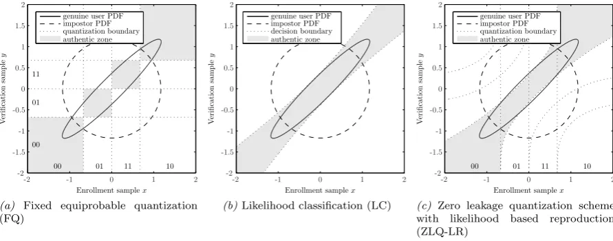
(a) Fixed equiprobable quantization (FQ)

Enrollment samplex

V er ifi ca tio n sa m p le y

genuine user PDF impostor PDF decision boundary authentic zone

-2 -1 0 1 2 -2 -1.5 -1 -0.5 0 0.5 1 1.5 2

(b)Likelihood classification (LC)

00 01 11 10

Enrollment samplex

V er ifi ca tio n sa m p le y

genuine user PDF impostor PDF quantization boundary authentic zone

-2 -1 0 1 2 -2 -1.5 -1 -0.5 0 0.5 1 1.5 2

(c) Zero leakage quantization scheme with likelihood based reproduction (ZLQ-LR)

Figure 6: Quantization and decision patterns based on the genuine user and impostor PDFs. Ideally the genuine user PDF should be contained in the authentic zone and the impostor PDF should have a large mass outside the authentic zone. 50% probability mass is contained in the genuine user and impostor PDF ellipse and circle. The genuine user PDF is based on a 10 dB SNR.

4

Optimal Reconstruction

The goal of the HDS reconstruction algorithm Rep(y, w) is to reliably reproduce the secrets. The best

way to achieve this is to choose the most probable ˆsgivenyandw, i.e., a maximum likelihood algorithm.

Lemma 4.1:Let Rep(y, w) be the reproduction algorithm of a ZL FE system. Letg−1

s be the inverse

of the helper data generation function for a given secrets. Then optimal reconstruction is achieved by

Rep(y, w) = arg max

s∈S

fY|X(y|g−s1(w)). (38)

Proof. As noted above, optimal reconstruction can be done by selecting the most likely secret giveny, w,

Rep(y, w) = arg max

s∈S fS|Y,W(s|y, w) (39)

= arg max

s∈S

fY,S,W(y, s, w)

fY,W(y, w)

. (40)

The denominator does not depend ons, and can hence be omitted. This gives

Rep(y, w) = arg max

s∈S fS,Y,W(s, y, w) (41)

= arg max

s∈S

fY|S,W(y|s, w)fW|S(w|s)ps. (42)

We constructed the scheme to be ZL, and therefore ps = 1/N and fW|S(w|s) = fW(w). We see that

bothpsandfW|S(w|s) do not depend ons, which implies they can be omitted from Eq. (42), yielding

Rep(y, w) = arg max

s∈S fY|S,W(y|s, w). (43)

Finally, knowingSandW is equivalent to knowingX. HencefY|S,W(y|s, w) can be replaced byfY|X(y|x)

withxsatisfyingQ(x) =sand g(x) =w. The uniquexvalue that satisfies these constraints isg−1

s (w).

To simplify the verification phase we can identify thresholdsτsthat denote the lower boundary of a

decision region. If τs≤ y < τs+1, we reconstruct ˆs=s. The τ0 =−∞and τN =∞ are fixed, which

implies we have to find optimal values only for theN₋1 variablesτ1, . . . , τN−1 as a function ofw.

Theorem 4.2:LetfY|X be a symmetric fading noise. Then optimal reconstruction in a FE scheme is

obtained by the following choice of thresholds

τs=λ

g−1

s (w) +g−s−11(w)

Proof. In case of symmetric fading noise we know that

fY|X(y|x) =ϕ(|y−λx|), (45)

withϕsome monotonic decreasing function. Combining this notion with that of Eq. (38) to find a point

y=τs that gives equal probability forsands−1 yields

ϕ(|τs−λg−s−11(w)|) =ϕ(|τs−λg−s1(w)|). (46)

The left and right hand side of this equation can only be equal for equal arguments, and hence

τs−λg−s−11(w) =±(τs−λg−s1(w)). (47)

Sinceg−1

s (w)6=g−s−11(w) the only viable solution is Eq. (44).

Instead of storing the ZL helper data w according to (36), one can also store the set of thresholds

τ1, . . . , τN−1. This contains precisely the same information, and allows for quicker reconstruction ofs:

just a thresholding operation on y and the τs values, which can be implemented on computationally

limited devices.

4.1

Special Case: 1-bit Secret

In the case of a one-bit secret s, i.e., N = 2, the above ZL FE scheme is reduced to storing a single

thresholdτ1.

It is interesting and somewhat counterintuitive that this yields a threshold for verification that does

not leak information about the secret. In case the average ofX is zero, one might assume that a positive

threshold value implies s = 0. However, boths = 0 and s = 1 allow positive as well as negative τ1,

dependent on the relative location ofxin the quantization interval.

4.2

FE: Equivalent choices for the quantization

Let us reconsider the quantization function Q(x) in the case of a Fuzzy Extractor. Let us fix N and

take theg(x) as specified in Eq. (37). Then it is possible to find an infinite number of different functions

Q that will conserve the ZL property and lead to exactly the same error rate as the original scheme.

This is seen as follows. For any w_∈[0,1) there is an N-tuplet of sibling points. Without any impact

on the reconstruction performance we can permute the s-values of these points; the error rate of the

reconstruction procedure depends only on the x-values of the sibling points, not on the s-label they

carry. It is allowed to do this permutation for everywindependently, resulting in an infinite equivalence

class of Q-functions. The choice we made in Section 2 yields the simplest function in an equivalence

class.

5

Example: Gaussian features and BCH codes

To be able to benchmark the reproduction performance of our scheme we will give an example based on Gaussian-distributed variables. In this example we will assume all variables to be Gaussian distributed, although the scheme is capable of achieving optimal reproduction for any kind of random variable with a fading noise distribution. The results in this example are obtained by numerical integration of the genuine user PDF given the corresponding scheme’s thresholds.

We will compare the reproduction performance of our Zero Leakage Quantization scheme with Like-lihood based Reproduction (ZLQ-LR) to a scheme with 1) Fixed Quantization (FQ) and 2) LikeLike-lihood Classification (LC). The former is, to our knowledge, the only other scheme sharing the zero secrecy leakage property, since this scheme does not use any helper data. Instead fixed quantization intervals are defined for both enrollment and verification as explained in section 1.5.1. An example of such a

quanti-zation withN = 4 intervals is depicted in Fig. 6a. Likelihood classification is not an actual quantization

scheme since it requires the enrollment sample to be stored in-the-clear. However, a likelihood based classifier provides an optimal trade-off between false accept and false reject according to communication theory [5] and should therefore yield the lowest error rate one can get. Instead of quantization boundaries the classifier is characterized by decision boundaries as depicted in Fig. 6b.

A comparison with QIM cannot be made since the probability for an impostor in a QIM scheme

Signal-to-Noise ratio [dB]

R

ec

o

n

st

ru

ct

io

n

er

ro

r

p

ro

b

a

b

ilit

y

N

= 4

FQ

ZLQ-LR

LC

0

5

10

15

20

10

10

10

10

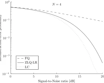
10

Figure 7: Reproduction performance in terms of error probability for Gaussian distributed features and Gaussian noise forN = 4.

comparison since the other schemes are designed to possess this property. Moreover, the QIM scheme allows the reproduction error probability to be made arbitrary small by increasing the quantization width at the cost of leakage.

Also the likelihood based classification can be tuned by setting the a decision threshold. However,

for this scheme it is possible to choose a threshold such that an impostor will have a probability of 1/N

to be accepted, which corresponds to the 1/N probability of correctly guessing the enrolled secret in a

fuzzy extractor scheme. Note that for a likelihood classifier there is no enrolled secret since this is not a quantization scheme.

As can be seen from Fig. 7, the reproduction performance for a ZSL scheme with likelihood based reproduction is always better than that of a fixed quantization scheme. However, it is outperformed by the likelihood classifier. Differences are especially apparent for features with a higher signal-to-noise ratio. In these regions the fixed quantization struggles with a inherent high error probability, while the ZSL scheme follows the likelihood classification.

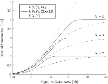
In a good quantization scheme there needs to be a small gap between the mutual informationI(X;Y)

andI(S; ˆS). For a Gaussian channel standard expressions are known from [5, Eq. (9.16)]. The mutual

information I(S; ˆS) can be calculated by using the numerical evaluation for the error probability as

described above. Fig. 8 show that a fixed quantization requires a higher SNR to converge to the maximum number of bits, whereas the ZLQ-LR scheme directly reaches this value.

Finally, we will consider the vector case of the two quantization schemes discussed above. In this section we concluded that the fixed quantization will have a larger error probability during reproduction, but we will show how this relates to either false rejection of genuine users or secret length when combined with a code offset method using error correcting codes [9].

In order to derive these properties we will assume the features to be i.i.d. and therefore we can calculate false acceptance rate (FAR) and false rejection rate (FRR) based on a binomial distribution. In practice features can be made (nearly) independent, but they will in general not be identically distributed. However, results will be similar. Furthermore we assume the error correcting code can be applied such that its error correcting properties can be fully exploited. This implies we have to use a gray code to label the extracted secrets before concatenation.

Signal-to-Noise ratio [dB]

M

u

tu

a

l

In

fo

rm

a

tio

n

[b

it

s]

N

= 2

N

= 4

N

= 8

I

(S

; ˆ

S

), FQ

I

(S

; ˆ

S

), ZLQ-LR

I

(X

;

Y

)

-10

0

10

20

30

40

0

0.5

1

1.5

2

2.5

3

3.5

4

Figure 8: Mutual information between S andSˆ for Gaussian distributed features and Gaussian noise.

omit one bit. For analysis we have also included the code (127,127,0), which is not an actual code, but

represents the case in which no error correction is applied.

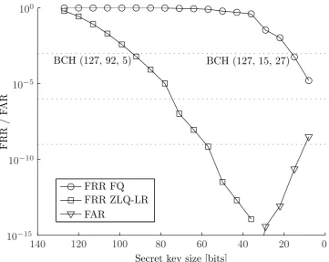
Suppose we want to achieve a target FRR of 1·10−3_{, the topmost dotted line in Fig. 9, then we}

require a BCH (127,92,5) code for the ZSL-LR scheme, while a BCH (127,15,27) code is required for the

fixed quantization scheme. This implies we would have a secret key size of either 92 or 15 bits. Clearly the last will not be sufficient for any security application since it has a key size that can be attacked in a limited amount of time. At the same time, due to the small key size, the scheme has an increased FAR as depicted in Fig. 9.

6

Conclusion

In this paper we have studied a generic Helper Data Scheme (HDS) which comprises the Fuzzy Extractor (FE) and the Secure Sketch (SS) as special cases. In particular, we have looked at the Zero Leakage (ZL)

property of HDSs in the case of a one-dimensional continuous sourceX and continuous helper dataW.

We make minimal assumptions, justified by Conjecture 3.4: we consider only monotonic g(x). We

have shown that the ZL property implies the existence of sibling points _{xsw}s∈S for every w. These

are values ofxthat have the same helper data w. Furthermore, the ZL requirement is equivalent to a

quantile relationship (Theorem 3.6) between the sibling points. This directly leads to equation (36) for

computingwfrom x. (Applying any reversible function to thiswyields a completely equivalent helper

data system.) The special case of a FE (ps= 1/N) yields them→ ∞limit of the Verbitskiy et al. [19]

construction.

We have derived reconstruction thresholdsτsfor a ZL FE that minimize the error rate in the

recon-struction ofs(Theorem 4.2). This result holds under very mild assumptions on the noise: symmetric and

fading. Eq. (44) contains the attenuation parameterλ, which follows from the noise model as specified

in Section 2.2.

BCH (127, 15, 27)

BCH (127, 92, 5)

Secret key size [bits]

F

R

R

/

F

A

R

FRR FQ

FRR ZLQ-LR

FAR

0

20

40

60

80

100

120

140

10

10

10

10

Figure 9: System performance compared to a scheme applying fixed quantization.

References

[1] M. Abramowitz and I. A. Stegun.Handbook of Mathematical Functions with Formulas, Graphs, and

Mathematical Tables, 9th printing. Dover, New York, 1972.

[2] B. Chen and G. Wornell. Quantization index modulation: a class of provably good methods for

digital watermarking and information embedding. Information Theory, IEEE Transactions on,

47(4):1423 –1443, may 2001.

[3] C. Chen, R. N. J. Veldhuis, T. A. M. Kevenaar, and A. H. M. Akkermans. Multi-bits biometric

string generation based on the likelihood ratio. InBiometrics: Theory, Applications, and Systems,

2007. BTAS 2007. First IEEE International Conference on, pages 1–6, 2007.

[4] M. H. M. Costa. Writing on dirty paper (corresp.). Information Theory, IEEE Transactions on,

29(3):439–441, 1983.

[5] T. M. Cover and J. A. Thomas. Elements of Information Theory. John Wiley & Sons, Inc., second

edition, 2005.

[6] J. A. de Groot and J.-P. M. Linnartz. Improved privacy protection in authentication by fingerprints. InProc of the 32st Symp on Inf Theory in the Benelux, 2011.

[7] Y. Dodis, L. Reyzin, and A. Smith. Fuzzy extractors: How to generate strong keys from biometrics

and other noisy data. InLNCS. Springer, 2004.

[8] D. Holcomb, W. Burleson, and K. Fu. Power-Up SRAM State as an Identifying Fingerprint and

Source of True Random Numbers.Computers, IEEE Transactions on, 58(9):1198 –1210, sept. 2009.

[9] A. Juels and M. Wattenberg. A fuzzy commitment scheme. In CCS ’99: Proceedings of the 6th

ACM conf on Comp and comm security, 1999.

[10] E. Kelkboom, K. de Groot, C. Chen, J. Breebaart, and R. Veldhuis. Pitfall of the detection rate

optimized bit allocation within template protection and a remedy. InBiometrics: Theory,

[11] E. Kelkboom, G. Molina, J. Breebaart, R. Veldhuis, T. Kevenaar, and W. Jonker. Binary biometrics:

An analytic framework to estimate the performance curves under gaussian assumption. Systems,

Man and Cybernetics, Part A: Systems and Humans, IEEE Transactions on, 40(3):555 –571, may 2010.

[12] J.-P. Linnartz and P. Tuyls. New shielding functions to enhance privacy and prevent misuse of

biometric templates. InAudio- and Video-Based Biometric Person Authentication. Springer, 2003.

[13] F. MacWilliams and N. Sloane.The Theory of Error Correcting Codes. North-Holland Mathematical

Library. North-Holland, 1978.

[14] T. Matsumoto, H. Matsumoto, K. Yamada, and S. Hoshino. Impact of artificial “gummy” fingers on

fingerprint systems. Optical Security and Counterfeit Deterrence Techniques, 4677:275–289, 2002.

[15] G. E. Suh and S. Devadas. Physical unclonable functions for device authentication and secret key

generation. InProceedings of the 44th annual Design Automation Conference, DAC ’07, pages 9–14,

New York, NY, USA, 2007. ACM.

[16] P. Tuyls, A. Akkermans, T. Kevenaar, G.-J. Schrijen, A. Bazen, and R. Veldhuis. Practical biometric

authentication with template protection. InAudio- and Video-Based Biometric Person

Authenti-cation, pages 436–446. Springer, 2005.

[17] P. Tuyls, B. ˇSkori´c, and T. Kevenaar. Security with Noisy Data: Private Biometrics, Secure Key

Storage and Anti-Counterfeiting. Springer-Verlag New York, Inc., Secaucus, NJ, USA, 2007.

[18] T. van der Putte and J. Keuning. Biometrical fingerprint recognition: don’t get your fingers burned. InFourth Working Conference on Smart Card Research and Advanced Applications, pages 289–303, Norwell, MA, USA, 2001. Kluwer Academic Publishers.

[19] E. A. Verbitskiy, P. Tuyls, C. Obi, B. Schoenmakers, and B. ˇSkori´c. Key extraction from general

nondiscrete signals.Information Forensics and Security, IEEE Transactions on, 5(2):269 –279, June

2010.

[20] B. ˇSkori´c, P. Tuyls, and W. Ophey. Robust key extraction from physical uncloneable functions.

In J. Ioannidis, A. Keromytis, and M. Yung, editors,Applied Cryptography and Network Security,

volume 3531 of Lecture Notes in Computer Science, pages 99–135. Springer Berlin / Heidelberg,

2005.

[21] J. L. Wayman, A. K. Jain, D. Maltoni, and D. Maio, editors.Biometric Systems: Technology, Design