Solving Nonlinear Least Squares Problem Using Gauss-Newton
Method
Wen Huey Lai1, Sie Long Kek2 and Kim Gaik Tay3 1
Department of Mathematics and Statistics, Universiti Tun Hussein Onn Malaysia, Batu Pahat, Johor, Malaysia
2
Center for Research on Computational Mathematics, Universiti Tun Hussein Onn Malaysia, Batu Pahat, Johor, Malaysia
3
Department of Communication Engineering, Universiti Tun Hussein Onn Malaysia, Batu Pahat, Johor, Malaysia
Abstract
For a nonlinear function, an observation model is proposed to approximate the solution of the nonlinear function as closely as possible. Since the parameters in the model are unknown, a successive approximation scheme is required. In this study, the Gauss-Newton algorithm is derived briefly. In doing so, a residual between the nonlinear function and the model proposed is constructed, and the sum squares of error (SSE) is then minimized. During the computational procedure, the gradient equations are calculated. By taking the gradient equation equals to zero and doing some algebraic manipulations, the normal equations are resulted. These normal equations are the basis for constructing the Gauss-Newton algorithm. For illustration, nonlinear least squares problems with nonlinear model proposed are solved by using the Gauss-Newton algorithm. In conclusion, it is highly recommended that the iterative procedure of the Gauss-Newton algorithm gives the best fit solution and its efficiency is proven.
Keywords: Gauss-Newton Method, Sum of Squares Error,
Parameter Estimation, Jacobian matrix, Iteration Calculation.
1. Introduction
In a statistical model, the unknown parameters can be estimated by using maximum likelihood estimation and least squares approach [1]. For these methods, the method of least squares is a standard method to approximate the solution of over determined systems. Least squares is defined that the overall solution minimizes the sum squares of error (SSE) made in the results of every single equation. The first clearly and brief presentation of the method of least square was published by Legendre in 1805 [2]. Nonetheless, Gauss declared that this method had been used before that of proposing by Legendre [3]. Basically, least squares problems are divided into linear and nonlinear least squares problems, depending on the linearity of the model used and the corresponding unknown parameters. This method of least squares is most commonly used in curve fitting. The reason is that the best
fit in the least-squares sense minimizes the SSE which is the difference between the observed value and the fitted value provided by the model used [4]. The SSE is used instead of the offset absolute values because the value of SSE allows the residuals to be treated as a continuous differentiable quantity. Minimizing SSE as the objective function can be justified by consistency of the optimization method. The approaches for solving nonlinear least squares problems include Gauss-Newton method, Newton’s method, Quasi-Newton method, and Levenberg-Marquardt method are well-defined [5].
2. Problem Statement
3. Gauss-Newton Method
An optimization problem occurs when an objective function is, either minimized or maximized, over a set of constraints. In our study, the nonlinear least squares problem is formulated as an optimization problem without constraints, where the SSE is defined as an objective function. During the computation procedure, the SSE is minimized, whereas the unknown parameters in the proposed model are determined in the optimal sense [5]. Here, the nonlinear least squares problem, which is an unconstraint optimization problem, is defined by
T 2
1
1 1
min ( ) ( ) ( ) ( ( ))
2 2
n
m
i x
i
f x r x r x r x
∈ℜ = =
∑
= (1)where f x( ) :ℜ → ℜn is the objective function, and r xi( )
is the residual function, which is defined by
( ) ( , ) , 1, 2,..., ,
i i i
r x =
φ
t x −y i= m (2)where
φ
( , )t xi is the proposed function and yi is theobservation data. The gradient of f x( ) is given by
T
( ) ( ) ( )
g x =J x r x (3)
where J x( ) is the Jacobian matrix of the residual function
( )
r x . The Hessian matrix is given by
T 1
( ) ( ( ) ( ) ( )) m
i i i
i
G x S x r x r x
=
=
∑
+ ∇ ∇ (4)where
S x( )= ∇2r x r x( ) ( ). (5)
Now, write the objective function f x( ) as the second order Taylor series expansion, which is the quadratic model, as follows:
T
T 2
1
( ) ( ) ( ) ( ) ( )( )
2 1
( ( ) ( ) ( ))( ) .
2
T
k k k k k
k k k k
q x r x r x J x r x x x
S x J x J x x x
= + −
+ + −
(6)
Notice that differentiate (6) with respect to x and let it equal to zero, we have
T T
( k) ( k) ( ( k) ( k) ( k))( k) 0
J x r x + S x +J x J x x−x = . (7)
Rearrange (7), the following normal equation is obtained:
T T
( (S xk)+J x( k) J x( k))(x−xk)= −J x( k) r x( k). (8)
After some algebra manipulations, let x=xk+1, then (8) becomes
T 1 T 1 ( ( ) ( ) ( )) ( ) ( )
k k k k k k k
x + =x − S x +J x J x − J x r x . (9)
By neglecting the term S x( ), the Gauss-Newton recursion equation is resulted as follows:
1
k k k
x + =x +s (10) with
T 1 T
( ( ) ( )) ( ) ( )
k k k k k
s = − J x J x − J x r x . (11)
From the discussion above, the computation procedure of the Gauss-Newton algorithm is summarized as follows.
Algorithm 1: Gauss-Newton Algorithm
Step 0 Set starting values of x0, tolerance
ε
>0,and k=0.
Step 1 Compute the residual function r xi( k), 0,i= , ,m from (2).
Step 2 Calculate the Jacobian matrices J x( k),
T
( k) ( k)
J x J x and ( (J xk)TJ x( k)) 1
− .
Step 3 Calculate the gradient gk =g x( k) from (3). If
||gk|| ≤
ε
, stop.Step 4 Calculate sk from (11).
Step 5 Update xk+1=xk+sk from (10). Set k = k + 1, and go to Step 1.
Remarks:
(a) For the accuracy purpose, the value of the
tolerance is chosen as small as possible. (b) The initial value x0 is chosen arbitrarily. (c) The inverse of the matrix ( (J xk)TJ x( k)) 1
− exist
during the calculation procedure.
4. Results and Discussion
parameters are determined in which to give the least value of the SSE. Then, the fitted line of each model and the original data are presented.
4.1 Example 1: Exponential Data
Given a set of data points ( ,t yi i)as below [6]:
Table 1: Observations
t y
1 10
2 5.49
3 0.89
4 -0.14
5 -1.07
6 0.84
The function
1exp( 2)
y=x − ⋅t x
is proposed to fit the data in Table 1. By using the initial guesses
(0) 1 10
x = and x2(0)=0.001,
the following model is obtained:
25.487 exp( 0.904 )
y= − ⋅t
where the final values of x1 and x2 are 25.487041 and 0.904330, respectively. From the calculation result, the value of SSE is 5.490956 with 22 iteration steps. The Jacobian is
1 2
(−tx exp(−tx ), exp(−tx2))T.
The graph of the data points and the model proposed is shown in Fig. 1.
1 1.5 2 2.5 3 3.5 4 4.5 5 5.5 6
-2 0 2 4 6 8 10 12
t
y
Fig. 1 Curve fitting for observation.
4.2 Example 2: Sinusoidal Data
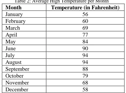
A list of average monthly high temperatures for the city of Monroe Louisiana [7] is given below:
Table 2: Average High Temperature per Month
Month Temperature (in Fahrenheit)
January 56
February 60
March 69
April 77
May 84
June 90
July 94
August 94
September 88
October 79
November 68
December 58
The relation between the temperature (yi) and the month (ti ) would be determined. For convenience, we label January as 1, February as 2, and so forth. The function
1 2 3 4
( ) sin( )
y t =x x t+x +x
is proposed. With the initial guesses
(x1(0),x(0)2 ,x3(0),x4(0)) = (15, 0.4, 10, 1),
1 2
3 4
19.898335, 0.475806, 10.771250, 74.500317.
x x
x x
= =
= =
The algorithm takes 16 number of iterations to converge. The Jacobian is
(sin(x t2 +x3), tx1cos(x t2 +x3), x1cos(x2+x3), 1)T.
The model obtained is
( ) 19.898 sin(0.476 10.771) 74.5
y t = ⋅ ⋅ +t + .
The fitted line of the model proposed and the observed data are shown in Fig. 2.
0 2 4 6 8 10 12
55 60 65 70 75 80 85 90 95
t
y
Fig. 2Curve fitting for temperature per month.
4.3
Example 3: Model Validity
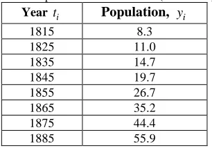
A set of data for the population (in millions) in the United States and the corresponding year [8] is used to discuss the model selection with curve fitting.
Table 3: Population of United States (in millions)
Year ti Population, yi
1815 8.3
1825 11.0
1835 14.7
1845 19.7
1855 26.7
1865 35.2
1875 44.4
1885 55.9
For convenience, 1815 is labeled as 1, 1825 as 2, and so forth. Next, three models are proposed, which are:
(a) y t( )=x t1 +x2, (b) y t( )=x1exp(x t2 ), and (c) y t( )=x t12+x2.
Taking the initial guesses for x1and x2 as 6 and 0.3, respectively, for these models, and after running the algorithm, the optimal parameter values for the respective model are given by
(a) x1=6.770238andx2 = −3.478571, (b) x1=7.000152 and x2=0.262077, (c) x1=0.751331andx2=7.828571.
Hence, the models proposed are
(a) ( )y t =6.770⋅ −t 3.479, (b) ( )y t =7.000 exp(0.262 )⋅ ⋅t
(c) y t( )=0.751⋅ +t2 7.829.
The respective Jacobians are
(a) J1 =(t, 1)T,
(b) J2 = (exp(x2 ⋅t), tx1 exp(x2 ⋅t))T,
(c) J3 = (t2, 1)T.
The values of SSE for the respective model used are
(a) 90.451548, (b) 6.013081, and (c) 0.312430.
As a result, Model (c) is the best model to be selected to fit with the real data given in Table 3. The plotting of the data points and these three models are shown in Fig. 3.
1 2 3 4 5 6 7 8
0 10 20 30 40 50 60
t
y
Actual Data (a) (b) (c)
Fig. 3 Comparison of Plotting between Three Models and the Actual
5.
Conclusions
The iterative algorithm of the Gauss-Newton method that is used for solving the nonlinear least squares problem was discussed in this paper. In general, it is typically difficult to decide an appropriate nonlinear function for a set of data. However, the model could be determined by observing the trend of the plotting of the data points. Then, the model proposed could be used to perform the curve fitting. In this study, the unknown parameters were determined by using the Gauss-Newton method, where the value of SSE was minimized. The calculation was started from an initial point, and at each iteration step, a step-size was computed. During the iteration procedure, the value of the unknown parameters was then updated. The iteration stopped when the convergence was achieved within a given tolerance. The parameter value with the minimum SSE is known as the optimum solution. For illustration, three examples were discussed. The results showed that the model proposed approximates closely to the actual data. In conclusion, the efficiency of the Gauss-Newton algorithm has been proven.
Acknowledgments
The authors would like to thank the Universiti Tun Hussein Onn Malaysia (UTHM) for financial supporting to this study under Incentive Grant Scheme for Publication (IGSP) VOT. U417.
References
[1]J. P. Hoffmann, Linear Regression Analysis: Applications and Assumptions. 2nd Ed. United States of America: Department of Sociology Brigham Young University, 2010.
[2]M. Merriman, “On the History of the Method of Least Squares”, The Analyst,Vol. 4, No. 2, 1877, pp. 33-36.
[3]S. M. Stigler, “Gauss and the Invention of Least Squares”, the Annals of Statistics, Vol. 9, No. 3, 1981, pp. 465-474.
[4]T. Kariya and H. Kurata, Generalized Least Squares. Great Britain: John Wiley & Sons, Ltd, 2004.
[5]J. Eriksson, (1996). “Optimization and Regularization of Nonlinear Least Squares Problems”, Ph.D. thesis, Umea University.
[6]G. Recktenwald, “Least Squares Fitting of Data to a Curve”, Department of Mechanical Engineering, Portland State University, 2001.
[7]T. Wherman, Applications of the Gauss-Newton Method. Retrieved Oct 22, 2015 from https://ccrma.stanford.edu
[8]A. Croeze, L. Pittman and W. Reynolds, Nonlinear Least-Squares Problems with the Gauss-Newton and Levenberg-Marquardt Methods. Retrieved May 21, 2015 from https://www.math.lsu.edu_system_files_MunozGroup1– Presentation.
Wen Huey Lai received the Bachelor degree in industrial statistics from the Universiti Tun Hussein Onn Malaysia, Johor, Malaysia, in 2016.
Sie Long Kek received the M.Sc. degree and the Ph.D. in mathematics from the Universiti Teknologi Malaysia, Johor, Malaysia, in 2002 and 2011, respectively. He is currently a Senior Lecturer in the Department of Mathematics and Statistics, Universiti Tun Hussein Onn Malaysia. His research interests includes optimization and control, operation research and management science, and modelling and simulation.
Kim Gaik Tay received the M.Sc. degree and the Ph.D. degree in mathematics from the Universiti Teknologi Malaysia, Johor, Malaysia, in 2000 and 2007, respectively. She is currently an Associate Professor in the Department of Communication Engineering, Universiti Tun Hussein Onn Malaysia. Her research interests includes nonlinear waves, optical