R E S E A R C H
Open Access
CP decomposition approach to blind
separation for DS-CDMA system using a new
performance index
Awatif Rouijel
1*, Khalid Minaoui
1, Pierre Comon
2and Driss Aboutajdine
1Abstract
In this paper, we present a canonical polyadic (CP) tensor decomposition isolating the scaling matrix. This has two major implications: (i) the problem conditioning shows up explicitly and could be controlled through a constraint on the so-called coherences and (ii) a performance criterion concerning the factor matrices can be exactly calculated and is more realistic than performance metrics used in the literature. Two new algorithms optimizing the CP
decomposition based on gradient descent are proposed. This decomposition is illustrated by an application to direct-sequence code division multiplexing access (DS-CDMA) systems; computer simulations are provided and demonstrate the good behavior of these algorithms, compared to others in the literature.
Keywords: CP decomposition; Tensor; DS-CDMA; Blind separation; Optimization
1 Introduction
Blind source separation consists in estimating unknown signals observed from their mixture without knowing any information about them, except mild properties such as their independence. Early work on blind source separa-tion was initiated by Jutten and Hérault [1,2] in the case of an instantaneous mixture. More recently, the use of multi-linear algebra methods has attracted attention in several areas such as data mining, signal processing, and partic-ularly in wireless communication systems, among others. Wireless communication data can sometimes be viewed as components of a high-order tensor (order strictly larger than 2). Solving the problem of source separation then means finding a decomposition of this tensor and deter-mining its parameters. One of the most popular tensor decompositions is the canonical polyadic decomposition (CP), also known as parallel factor analysis (PARAFAC), which can be seen as an analog of the matrix singular value decomposition (SVD), since it decomposes the tensor into a sum of rank-one components [3-5]. This decomposi-tion has been exploited and generalized in several works
*Correspondence: [email protected]
1Mohammed V-Agdal University, LRIT Associated Unit to the CNRST-URAC N29, Avenue des nations unies, Agdal, BP. 554 Rabat-Chellah, Morocco Full list of author information is available at the end of the article
for solving different signal processing problems [6,7] such as multi-array multi-sensor signal processing. The inter-est of the CP decomposition lies in its uniqueness under certain conditions. Typical algorithms for finding the CP components include alternating least squares (ALS) and descent algorithms [8,9], which do not isolate the scaling factor matrix. Herein, we propose two new optimization algorithms for CP tensor decomposition, which isolate the scaling matrix in the optimization process and offers the possibility to monitor the conditioning.
It is well known that loading matrices are identified up to column scaling. This indeterminacy is complicated to take into account, given that the product of all scaling matrices must be equal to the identity. For this reason, only approximate performance indices have been used so far by ignoring the last constraint. However, one can ask oneself whether it is possible to calculate the exact perfor-mance index: this is our second contribution. The present paper develops preliminary results appeared in [10] and includes performances obtained in the frame of direct-sequence code division multiplexing access (DS-CDMA) blind multiuser detection and estimation.
The rest of this paper is organized as follows. Section 2 presents notation, definitions, and properties of third-order tensors, and the exact CP decomposition problem is then stated. In Section 3, the low-rank approximation
is formulated. Existence and uniqueness of this decom-position are also investigated. ALS and the two proposed algorithms are presented in Section 4. Section 5 is dedi-cated to the new performance criterion with a focus on an exact performance index calculation. In Section 6, we show the usefulness of our algorithms and the perfor-mances obtained. An application of these algorithms to CDMA transmission is then provided to illustrate the effectiveness of the latter.
2 Notation and preliminaries 2.1 Notations and definitions
Let us first introduce some essential notation. Scalars are denoted by lowercase letters, e.g.,a. Vectors are denoted by boldface lowercase letters, e.g.,a; matrices are denoted by boldface capital letters, e.g.,A. Higher-order tensors are denoted by boldface Euler script letters, e.g., T. The pth column of a matrixAis denotedap, the(i,j)entry of a matrixAis denoted byAij, and element(i,j,k)of a third-order tensorT is denoted byTijk.1will represent a vector containing ones, andIthe identity matrix.
Definition 2.1.The scalar product of two same-sized tensorsX,YCI1×I2×···×IN is defined as:
X,Y = I1
i1=1
· · ·
IN
iN=1
Xi1,···,iNYi1,···∗ ,iN. (1)
where Xi1,···,iN is the(i1,· · ·, iN)elements of the Nthorder of tensor.
Definition 2.2.The outer (tensor) product between two tensor arraysX ∈ CI1×I2×···×IN andY ∈ CJ1×J2×···×JM of orders N and M, respectively, is denoted byZ = X⊗Y ∈
CI1×I2×···×IN×J1×J2×···×JMand defined by:
Zi1,···,iN,j1,···,jM =Xi1,···,iNYj1,···,jM. (2) The symbol ⊗ represents the tensor outer product. The outer product of two tensors is another tensor, the order of which is given by the sum of the orders of the two for-mer tensors. Equation 2 is a generalization of the concept of outer product of two vectors, which yields itself a matrix (second-order tensor). The outer product of three vectors a ∈ CI andb ∈ CJ andc ∈ CK yields a third-order decomposable tensorZ = a⊗b⊗c∈CI×J×K where Zijk = aibjck.
Definition 2.3.The rank of an arbitrary tensor T ∈
CI1×I2×...×IN, denoted by R = rank(X), is the mini-mal number of rank-1 tensors that yield T in a linear combination.
Decomposable tensors have thus a rank equal to 1.
Definition 2.4. The Kruskal rank, or krank, of a matrix is the largest number j such that every set of j columns is linearly independent.
Definition 2.5.The Frobenius norm of a tensor T ∈
CI1×I2×...×IN is defined as:
TF =
T,T. (3) Definition 2.6.The Khatri-Rao product between two matrices with the same number of columns, A = [a1, a2,· · ·,aF]∈ CI×F andB= [b1,b2,· · ·,bF]∈CJ×F, is defined as the column-wise Kronecker product:
AB=[a1b1,· · ·, aFbF]∈CIJ×F. (4) whereis the Kronecker product.
Definition 2.7.The coherence of a collection V =
{v1,· · ·,vr} of unit-norm vectors is defined as the maxi-mal value of the modulus of cross scalar products. In other words, the coherence of the collection V is defined as:
μV =max p =q|v
H
pvq|. (5)
Definition 2.8.Let A ∈ CI×J, then vec{A} ∈ CK denotes the column vector defined by:
(vec{A})i+(j−1)I=Aij. (6)
where K=IJ.
2.2 Preliminaries
A tensor of order d is an object defined on a product betweendlinear spaces. Once the bases of these spaces are fixed, a dthorder tensor can be represented by ad -way array (a hyper matrix) of coordinates [4]. The order of a tensor thus corresponds to the number of indices of the associated array. We are interested in decomposing a third-order tensorT as:
T =
R
r=1
λrD(r). (7)
where D(r) are decomposable tensors, that is, D(r) = ar⊗br⊗cr. Denote by( )Tmatrix transposition,λrreal pos-itive scaling factors,λ = [λ1,· · ·,λR]T, andRthe tensor rank. Vectors ar (resp. br andcr) live in a linear space of dimension I (resp. dimension J andK). Equivalently, decomposition (7) can be rewritten as a function of array entries:
Tijk = R
r=1
λrAirBjrCkr, i∈ {1,· · ·,I}, j∈ {1,· · ·,J}, k∈ {1,· · ·,K}.
where Air (resp.Bjr andCkr) denote the entries of vec-torar(resp.brandcr). The above decomposition is called the canonical polyadic decomposition (CP) of tensorT. The model (7) can be written in a compact form using the Khatri-Rao product, as:
TI,1KJ = A(CB)T, TJ,KI2 = B(CA)T, TK,JI3 = C(BA)T.
whereTI,KJ1 resp.TJ,KI2 andTK,3 JIis the matrix of size I×KJ (resp.J×KI andK ×JI) obtained by unfolding the arrayT of sizeI×J×K in the first mode (resp. the second mode and the third mode), andis theR×R diag-onal matrix defined as= Diag{λ1,. . ., λR}; see [5] for further details on matrix unfoldings.
The explicit handwriting of decomposable tensors as given in (8) is subject to scale indeterminacies. In the ten-sor literature, optimization of the CP decomposition (8) has been carried out without isolating the scaling factor, which is generally included in one of the loading matrices, so that=I. In [5], Kolda and Bader proposed to reduce the indeterminacies by normalizing the vectors and stor-ing the norms in. Our first proposal is to pull the factors
λroutside the product and calculate the optimal value of the scaling factor, which permits to monitor the condi-tioning of the problem. Scaling indeterminacies are then clearly reduced to unit modulus but are not completely fixed, hence the difficulty in estimating the identification error of loading matricesA,BandC. Our second proposal (Section 5) is to calculate the 3Rcomplex phases (reducing to signs in the real case).
3 Existence and uniqueness
The goal is to identify all parameters in the right hand side of (8), given the whole arrayT. According to exist-ing results [11-13], a third-order tensor (i.e., a three-way array) of rank R can be uniquely represented as sum of R rank-1 tensors, under certain conditions. Kruskal has demonstrated that the condition (9) is sufficient for uniqueness in CP decomposition [13], where kA is the krank of A. This means that matrices A, B, and C are unique up to permutation and (complex) scaling of their columns, under the Kruskal’s condition:
kA+kB+kC≥2R+2 (9)
For uniqueness, Harshman has shown that is sufficient to haveAandBof full rank, andCof krank ≥2 [3]. When 1 < R ≤ 2, the Kruskal and Harshman conditions are equivalent. ForR > 2, Kruskal’s condition may be satis-fied even when Harshman’s are not, and this condition is claimed to be only sufficient for R > 3 [14]. However, observations are actually corrupted by noise, so that (8) does not hold exactly.
3.1 Low-rank approximation
In practice, the exact CP decomposition always exists but with a very large rank. Hence, it may not be physically meaningful, and additionally, it is generally not unique. It is consequently preferred to fit a multi-linear model of lower rank,R<rankT, fixed in advance, so that we have to deal with an approximation problem. To estimate the parameters of the decomposition, we need to minimize the following cost function:
ϒ (A,B,C,)= T −(A,B,C).2F. (10) By convention (A,B,C). denotes the tensor of rank Rof coordinatesRr=1λrAirBjrCkr. Minimizing error (10) means finding the best rank-R approximate ofT and its CP decomposition. The cost function (10) can also be written in three equivalent compact forms with respect to the three loading matrices:
ϒ (A,B,C,) = TI,KJ1 −A(CB)T2 F,
= TJ,KI2 −B(CA)T2 F,
= TK,3 JI−C(BA)T2 F.
3.2 Conditioning of the problem
Assuming that the matricesA,B, andCare given, we will calculate the optimal value of the scaling factor. This can be done by expanding the Frobenius norm in (10), which is a quadratic form in the entries ofand canceling the gradient with respect toλ(see details in Appendix 1). Then, the following linear system is obtained:
Gλ=f, (11)
wherefis R-dimensional vector defined by the contrac-tionfr =ijkTijkAirBjrCkr,Grepresents theR×RGram matrix defined by:
3.3 Existence
According to the results in [15,16], the infimum of (10) may not be reachable. In fact, the set of tensors of rank at mostξis not closed ifξ >1. Examples of the lack of close-ness have been provided in the literature [15,16], which suffice to prove it. In other words, it may happen that for a given tensor, and for any rank-rapproximation of it, there always exists another better rank-rapproximation.
This is the reason why the authors proposed the con-straint below, which ensures existence of a minimum. Define the three coherencesμA,μB, and μC associated with the matricesA, B, andC, respectively. It has been indeed shown in [15,17] that under the constraint:
μAμBμC≤ 1
R−1, (13)
the infimum of (10) is reached. It may be seen that this condition already gives a quantitative bound to the condi-tioning of (11) because coherences bound extra-diagonal entries of matrixG, which has ones on its diagonal.
3.4 Uniqueness
The uniqueness of the tensor decomposition can be ensured by using a sufficient condition based on Kruskal’s theorem (9), previously mentioned.
According to the lemma reported in [17,18], an inequal-ity holds between Krank and coherence, namelykA≥ μ1A, as long askAis strictly smaller than the column rank of A. Including this inequality in Equation 9 leads to the following sufficient uniqueness condition:
μ−1A +μ−1B +μC−1≥2(R+1). (14)
4 Optimization for CP decomposition
In Section 3, we presented CP for three-way tensors. Various optimization algorithms exist to compute CP decomposition without constraint, as ALS or descent algorithms [7,8,19]. We subsequently present optimiza-tion algorithms to compute the CP decomposioptimiza-tion (10), under the constraints of unit norm columns of loading matrices.
4.1 Alternating least squares algorithm
The ALS algorithm was proposed for CP computation by Carroll and Chang in [20] and Harshman in [3] and still stays the workhorse algorithm today, mainly owing to its ease of implementation [21]. ALS is hence the classical solution to minimize the cost function (10), despite its lack of convergence proof. This iterative algorithm alternates among the estimation of matricesA,B, andC.
The principle of the ALS algorithm is to convert a non-linear optimization problem into three independent non-linear
least squares (LS) problems. In the first steps, one of the three matrices, say, A is updated while the two others (BandC) are fixed to their values obtained in previous estimation steps. The estimate ofAis given by:
A=TI,KJ
(CB)†
T
. (15)
whereTI,KJis the unfolding matrix of sizeI×JKdefined in Section 2.2, and()†is the Moore-Penrose pseudo inverse. By symmetry, the expressions are similar forBandC.
4.2 Proposed algorithms
Our optimization problem consists in minimizing the squared error ϒ under a collection of 3R constraints, namely:
min A,B,C,
T −
R
r=1
λrar⊗br⊗cr
2
F ,
ar = br = cr =1, 1≤r≤R
(16)
Therefore, we need to find three matrices A, B, and C of unit norm columns which minimize (16). Stack these three matrices in aI+J+KbyRmatrix denoted byX. The objective can now be also writtenϒ(X,), for the sake of convenience.
The computation of loading matrices is performed by minimizing the quadratic cost function (10). One gener-ates a series of itergener-atesX(k) = A(k)T,B(k)T, C(k)TT, k ∈ N, with initial valueX(0)arbitrarily chosen. Gener-ally, the algorithm consists of choosing at thekth iteration a point X(k +1) in a direction lying in the half space defined by the gradient of objective function ϒ, defined by matrixD(k), which verifies [22]:
vec{∇ϒ(X(k))}Tvec{D(k)}<0. (17) One possibility is to choose the direction opposite to the gradient:
D(k)= −∇ϒ(A(k),B(k),C(k)). (18) The gradient components∇ϒA(sizeI×R),∇ϒB(J×R), and∇ϒC (K×R) can be stacked into a single matrix of sizeI+J+KbyR:
D=
⎛ ⎝−∇−∇ϒϒAB
−∇ϒC
⎞
⎠. (19)
[23,24]. Using the quadratic form proposed in [23], the objective function can be expanded into:
ϒ (A,B,C;)= T2+ i
R
p=1 R
q=1
AipMpqA∗iq
−
i
⎛ ⎝R
q=1
NiqA∗iq+ R
p=1 AipNip∗
⎞ ⎠.
(20)
whereMpq = jkλpλ∗qBjpB∗jqCkpCkq∗ andNip = jkTijk
λ∗
pB∗jpC∗kp. Thus, the gradient ofϒwith respect toAis:
∂ϒ
∂A =2AM−2N. (21)
whereMof sizeR×RandNof sizeI×R. The gradient of
ϒwith respect toBandCis similar, taking into account the fact that matricesMandNneed to be defined accord-ingly (for the gradient ofϒ with respect toBandC, the dimension of matrixNisJ×RandK×R, respectively, while the dimension ofMis alwaysR×R).
The difficulty that arises in constrained optimization is to make sure that the move remains within the feasible set,C, defined by the constraints. In the following subsec-tions, we propose two versions of our algorithm, with two different ways of calculating scale factor.
Descent algorithms are also determined by the steps that will be executed in the chosen direction. There are various methods for the step selection, and the most widely used areBacktracking andArmijo [22]. To com-pute the stepsize (k) in Algorithm 1 and Algorithm 2, we use a popular inexact line search method, very simple and quite effective, which is the backtracking line search. It depends on two fixed constantsα,β with 0< α < 0.5 and 0< β <1.
Backtracking algorithm
1. Given a descent directionDforϒ,α∈(0, 0.5),
β∈(0, 1).
2. Initialization:=1.
3. whileϒ(X+D;) > ϒ(X;)+α∇ϒTD 4. =β.
4.2.1 Algorithm 1
In the recent work on CP tensor decomposition, opti-mization of the objective function (10) was made without explicitly considering the factor. More precisely in most contributions, the scaling factor is integrated into load-ing matrices, so that may be set to the identity. The first solution we propose is to use a projected gradient
algorithm while calculatingas the product of normaliz-ing factors of matricesA,B, andC:
(k)=(k−1)ABC. (22) whereis the Hadamard product,A=Diag{a1,· · ·,
aR}, and similar definitions for B and C. This approach, which we call ‘Algorithm 1’ can be described by the pseudo-code below:
1. Initialize{A(0);B(0);C(0)}to full-rank matrices with unit norm columns, and set(0)=I
2. Fork≥1and subject to a stopping criterion, do: (a) Compute the descent direction as the
gradient w.r.t.X:
D(k)= −∇ϒ(X(k−1);(k−1)), (b) Compute a stepsize(k)using the
backtracking method [22] such as:
ϒ(X(k−1)+(k)D(k);(k−1))
< ϒ(X(k−1);(k−1)). (c) UpdateX(k)=X(k−1)+(k)D(k) (d) Extract the three blocks ofX(k):A(k),B(k)
andC(k), and store the norm of their columns intoA,B,C
(e) Normalize them to unit-norm columns as:
A(k):=A(k)−1A ,B(k):=B(k)−1B , and C(k):=C(k)−1C (f) update(k)=(k−1)ABC
4.2.2 Algorithm 2
The other approach is to consideras an additional vari-able. By canceling the gradient ofϒ(X,)with respect to
, one obtains Equation 11, which can be solved for whenXis fixed. This gives the algorithms below.
Algorithm 2.
1. Initialize(A(0),B(0),C(0))to full-rank matrices with unit-norm columns.
2. ComputeG(0)andf(0), and solveG(0)λ=f(0)for
λ, as defined in Section 3.2 by (11). Set
(0)=Diag{λ}.
3. Fork≥1and subject to a stopping criterion, do (a) Compute the descent direction as the
gradient w.r.t.X:
D(k)= −∇ϒ(X(k−1);(k−1)) (b) Compute a stepsize(k)using the
backtracking method [22] such as:
ϒ (X(k−1)+(k)D(k);(k−1))
(c) UpdateX(k)=X(k−1)+(k)D(k) (d) Extract the three blocks ofX(k):A(k),B(k)
andC(k)
(e) Normalize the columns ofA(k),B(k)and C(k)
(f) ComputeG(k)andf(k), and solve G(k)λ=f(k)forλ, according to (11). Set
(k)=Diag{λ}.
Stopping criterion. The convergence is usually consid-ered to be obtained at thekth iteration when the error between tensorT, and the tensor reconstructed from the estimated loading matrices, does not significantly change between iterationskandk+1.
However, in the complex case, the phase of the entries of loading matrices found at the end of the algorithm – as defined by the stopping criterion above - is different from the original. To remedy this problem, we propose a new performance criterion in order to minimize the dis-tance between the original and the estimated matrices. Although this criterion is not usable when actual load-ing matrices are unknown, it still permits to assess the performances effectively attained.
5 Performance criterion
As highlighted in Section 2, there is always an indeter-minacy in the representation of decomposable tensors, characterized in the CP decomposition by 3R complex numbers of unit modulus. In order to better understand this problem, let a, b, and c denote the rth column of matricesA,B, andC, respectively, with 1 ≤ r ≤ R. Fur-thermore,a,ˆ b, andˆ cˆdenote one column of the estimated matrices entering in the CP decomposition. We seek to minimize a distance:
δx;xˆ = min ϕ,ψ,χ
a−ejϕaˆ2+b−ejψbˆ2+c−ejχcˆ2
.
(23)
In the literature, only approximate performance indices have been used so far by neglecting relation between the anglesϕ,ψandχgiven by:
exp(j (ϕ+ψ+χ))=1.
Our contribution herein consists in finding the exact minimum distance (23) under this angular constraint, by calculating the 3Roptimal phases affecting the columns of the estimated loading matrices.
The derivative of Equation 23 with respect toϕandψ yields a system of two equations. Finding 3Rphases means to solve, if the 2 sets of 3 columns are fixed:
ρasinx+ρcsin(ϕ+ψ+γ ) =0,
ρbsiny+ρcsin(ϕ+ψ+γ ) =0. (24)
wherex=ϕ−αandy=ψ−β. After some trigonometric manipulations described in Appendix 2, the solutions can be obtained by rooting a polynomial of degree 6 in a sin-gle variableϕ. By replacing the admissible values ofϕinto system (24), the corresponding values ofψ are obtained. The calculation of the minimum distance (23) is done for all possible permutations. We end up with the following performance criterion:
E(T;A,B,C,)=min π∈
R
r=1
δxr;xˆπ(r) . (25)
whereis the set of permutations of{1, 2,· · ·,R}. When the permutation acts in too large dimension, greedy ver-sions are possible to limit the exhaustive search in the permutation set.
Denoteπ(i)as the permutations of, 1≤i ≤R!. The overall algorithm to compute the performance criterion is summarized as follows:
1. For1≤i≤R!do
2. Calculate the3Roptimal phases affecting the columns of the estimated loading matrices:
(a) Permute the columns of the three estimated matrices according to the permutationπ(i):
Aπ(i),Bπ(i), andCπ(i);
(b) For eachrth columns of loading matrices and estimated matrices, do:
• Setx=ϕ−αandy=ψ−βand solve the polynomial of degree 6 in a single variableϕ:
c0 +c1cos(2x)+c2cos2(2x)+c3cos3(2x)
+c4cos4(2x)+c5cos5(2x)+c6cos6(2x)=0.
• Replacexinsiny= ρa
ρbsinx, obtainyand
consequentlyψ;
• Calculateχin:exp(j (ϕ+ψ+χ))=1;
• Calculate the minimum distanceδ:
δx;xˆ = min ϕ,ψ,χ
a−ejϕaˆ2+b−ejψbˆ2
+c−ejχcˆ2
.
• Save the results:distance(i)=δ,phaseϕ(i)=ϕ, phaseψ(i)=ψ andphaseχ(i)=χ;
3. End do.
4. Choose the3Rangles which return the smaller distanceδ.
6 Simulation results
and the second one for DS-CDMA system. In all exper-iments, the results are obtained from 100 Monte Carlo runs. At each iteration and for every SNR value, a new noise realization is drawn. The stopping criterion chosen for all experiments isϒ(n) < and|ϒ(n)−ϒ(n−1)|< , where is a threshold by which the global minimum is considered to be reached, andnis the current iteration. In the following simulations, we take:=10−6.
6.1 Example 1: random loading matrices
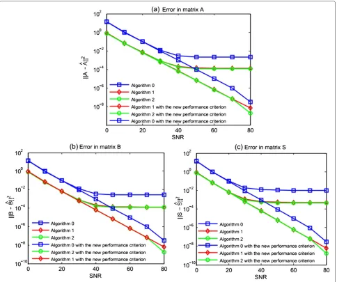
In order to illustrate the behavior and performances of the proposed algorithms, we first report simulation results run on random tensors. In a first stage, we compare ‘Algorithm 2’, ‘Algorithm 1’, and the gradient descent algo-rithm named herein ‘Algoalgo-rithm 0’. We will analyze the errors of matrix estimation obtained through the perfor-mance criterion proposed in Section 5. Two scenarios are analyzed using random tensors: (i) one tensor of rank 2 with dimensions 3×3×3 and (ii) another tensor of rank 5 with dimensions 8×8×8. Loading matrices are initial-ized with random-valued columns and the two tensors are corrupted by an additive Gaussian noise.
Figures 1 and 2 depict matrix estimation errors implied in (25) as a function of SNR. As expected, it can be seen that the results using Algorithm 0 show a poor per-formance when compared to the results obtained with Algorithms 1 and 2 (curves with diamonds and circles). This supports the idea that our algorithms isolating the scaling matrix are attractive. Furthermore, we check that when the phase constraints are neglected in the calcula-tion of the performance measure, the results are signifi-cantly more optimistic, particularly at high SNR (curves of the same color), which supports the interest of using our performance index defined in (5).
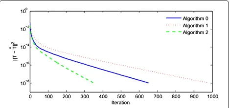
In order to show the significant difference between Algorithms 1 and 2, we will examine the convergence speed of the tensor reconstruction according to the num-ber of iterations, since the final error is about the same (cf. Figures 1 and 2). We consider the case of a 3×3×3 ten-sor of rank 2. The latter was constructed from three 3×2 Gaussian matrices drawn randomly. The results are pre-sented in Figure 3, and show that in all our experiments, Algorithm 2 converged faster in terms of number of iter-ations, while Algorithm 1 and Algorithm 0 require more iterations to reach convergence.
6.2 Example 2: application To DS-CDMA system
In this example, we place ourselves in a blind context. We assume that the receiver has no knowledge neither on the spreading codes nor on symbol sequences. Classi-cally, telecommunications blind techniques are based on somea prioriknowledge, such as temporal properties of transmitted signals or the spatial properties of the receiver [25-27].
Recently, algebraic tensor methods have received con-siderable attention in signal processing [2]. It also turns out that multilinear algebra tools are often more power-ful than their matrix equivalent. Sidiropoulos et al. are the first to adopt tensor approaches in the telecommunica-tions field in 2000 [12]. They observed that the samples of a CDMA signal received by an array of antennas can be stored in a cube, each dimension corresponding to a diversity (coding diversity, temporal diversity, and spatial diversity). Thus, they showed that the deterministic blind separation problem of CDMA signals can be solved by the CP decomposition [28].
In this example, we propose to apply the CP decompo-sition algorithms as detailed in Section 4 with the new performance criterion on the DS-CDMA technique. A comparison with the ALS algorithm is then made.
6.2.1 Tensor modeling
We considerRusers with one transmitting antenna, trans-mitting simultaneously their signals to an array of K receiving antennas. In other words, we consider a commu-nication system of type ‘multiuser SIMO’.
For example, assume the userrtransmits the symbols sr of size J. These symbols are spreaded by cr CDMA code of lengthI, uniquely allocated to userrand assumed to be unknown at the receiver. These codes are binary sequences taking values from{−1, 1}and could be non-orthogonal. The spreading sequence propagates along a single path in a memoryless channel and is received by the antenna array under angle of arrivalθr. Each of theK antennas receives a signalYk(t)of sizeJ×I. Our approach for detection and separation of the received signals is to exploit the multilinear algebraic structure of these signals using the new performance criterion. We observe these signals during a time span of lengthJTs, whereTs is the symbol period. TheYk(t)signals are sampled at the chip periodTc = Ts/I, whereIis the spreading factor. There-fore, each antenna provides a set ofIJ samples that can be ordered in a tensor of order 3, denotedY ∈ CI×J×K. TheYijkcomponent of this tensor that corresponds to the sample of the overall signal received by thekth antenna at timeiof thejth symbol period can be written as follows:
Yijk = R
r=1
AkrSjrCir i∈[1,I] j∈[1,J] k∈[1,K] . (26)
where the complex scalarAkr = βrak(θr), withβr is the fading coefficient of therth user andak(θr)the response of the antennakat the angle of arrivalθr.
Figure 1Matrix estimation errors, with a random tensor of size 8×8×8 and rank 5.(a)Matrix A.(b)Matrix B.(c)Matrix S.
Figure 3Typical example of reconstruction error (10) as a function of the number of iterations.For a tensor of size 3×3×3 and rank 5.
system. To calculate the CP decomposition ofY, we resort to Algorithm 2 presented in Section 4 with performance index (25). The detection and separation of the matrixS of transmitted symbols will be made, using the following objective function:
ϒ (A,C,S,)=
Y−
R
r=1
λrar⊗cr⊗sr
2
F
. (27)
wherear,cr, andsr are the normalized vectors; the scal-ing ambiguities on the estimated symbols are eliminated by normalizing each symbol sequence by its norm and calculating the exact scaling factor. As to correct the phases of the three estimated matrices, we will use the exact performance index (28) seen in Section 5.
E(T;A,C,S,)=min π∈
R
r=1
min ϕ,ψ,χ
ar−ejϕaˆπ(r)2
+cr−ejψcˆπ(r)2+sr−ejχsˆπ(r)2
.
(28)
6.2.2 Simulation
In this experiment, we present the performance of the receiver algorithms (Algorithm 1 and Algorithm 2 with new performance criterion) which estimate blindly the symbolS.
We considerR= 4 users communicate simultaneously in the same bandwidth. Each user transmits a sequence J = 20 of consecutive symbols and is uniquely assigned
Table 1 Angles of arrival for four users
Angles of arrival
Figure 4 (-60, -30, 0, 20)
Figure 4Bit error rate (BER) versus SNR results for scenario 1:
R=4,K=4,I=10, andJ=20.
a spreading sequence of lengthI =10. The user symbols are generated from an i.i.d distribution and are modulated using a pseudo-random quaternary phase shift keying (QPSK) sequence. The signal is transmitted to a receiver ofK = 4 antennas. The angles of arrival are described in Table 1.
In Figure 4, we will illustrate the ability of the blind ten-sorial receiver Algorithm 2 using the new performance criterion and the ALS receiver for noisy data extraction. Using Monte Carlo simulations, we will represent the evolution of bit error rate (BER) according to the signal-to-noise ratio (SNR). These results shown in Figure 4 indicate that the performance of the proposed receiver Algorithm 2 is better since it converges faster than the ALS algorithm. That is tied to the normalization of the factor matrices and the exact calculation of the scaling fac-tor. Moreover, we can see that BER of Algorithm 2 without the use of our criterion performance is very optimistic, which proves the interest of our study.
Table 2 Angles of arrival for three scenarios
Angles of arrival
Curve 1 ( -10, 20)
Curve 2 (-60, -40, 0, 20)
Curve 3 (-60,-50, 10, 40, 80)
The impact of factor KR, which represents the number of receiving antennas per user is illustrated in Figure 5. In this figure, curve 1 represents the case where the number of antenna isK = 4 and the number of users is R = 2, K=4, andR=4 for the second curve, while for the third curveK=2 andR=5. The angles of arrival are described in Table 2. As a result, the overall system performance is enhanced when increasing the factor KR, indicating the importance of spatial diversity.
7 Conclusions
In this paper, we have shown in Section 3.2 that, in CP tensor decompositions, the scale matrixtakes as opti-mal value a Gram matrix controlling the conditioning of the problem. This shows that bounding coherences would allow to ensure a minimal conditioning. We have described several algorithms able to compute the min-imal polyadic decomposition of three-way arrays. The two proposed algorithms Algorithm 1 and Algorithm 2 have been described and tested, which involve a sep-arate explicit calculation of the scale matrix . Con-trary to the performance measures used in the literature, which are optimistic by construction, the performance index calculated herein is more realistic by taking into account the angular constraint. An application of the CP decomposition with exact performance criterion to DS-CDMA system has been presented. Finally, computer simulations have been performed in the context of SIMO-CDMA system, in order to demonstrate both the good performances of the proposed algorithms, compared to ALS one and their usefulness in CDMA system. The judgment of our algorithms do not solely rely on the reconstruction error and the convergence speed, but it also takes into account the error in the loading matri-ces obtained and the BER in the case of the CDMA application.
Appendices Appendix 1
Detailedoptimal calculation
We intend to calculate the optimal value of which minimize the following expression:
ϒ(A,B,C,)= T −(A,B,C).2F. (29)
By developing, it leads to:
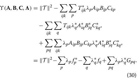
ϒ(A,B,C,)= T2− ijk
p
Tijk∗λpAipBjpCkp
−
ijk
q
Tijkλ∗qA∗iqB∗jqCkq∗,
+
pq
ijk
λpAipBjpCkpλq∗A∗iqB∗jqC∗kq,
= T2− p
λpfp∗−
q
λ∗qfq+
pq
λpλ∗qGpq.
(30)
whereGpq = ijkAipBjpCkpA∗iqB∗jqCkq∗ andfq=
ijkTijk A∗iqB∗jqCkq∗. By canceling the derivative ofϒwith respect to
λ, we find the following linear system:
Gλ=f. (31)
Appendix 2
Performance criterion details
In this appendix, we explain in more details how to obtain performance index δ, in particular how phases(ϕ,ψ,χ) are calculated. Settingχ = −ϕ−ψ [2π], equation (23) can be rewritten as:
δ = ||a||2+ ||ˆa||2+ ||b||2+ ||ˆb||2+ ||s||2+ ||ˆs||2
−2ρacos(ϕ−α)−2ρbcos(ψ−β)
−2ρscos(ϕ+ψ+γ ).
where aHaˆ def= ρaejα,bHbˆdef=ρbejβ andsHˆsdef=ρsejγ. Sta-tionary points are given by the solutions of the trigono-metric system ine.g.variablesx= ϕ−αandy=ψ −β as unknowns:
ρasinx+ρssin(ϕ+ψ+γ ) = 0,
ρbsiny+ρssin(ϕ+ψ+γ ) = 0. The first simplification is achieved by noting that
ρssin(ϕ+ψ+γ )= −ρasinx= −ρbsiny. implies
siny= ρa ρb
sinx.
Now, using trigonometric identities, we can rewrite the first equation of the trigonometric system
ρssin(ϕ+ψ+γ )=ρssin(x+y+α+β+γ )= −ρasinx. as
ρasinx = −ρs
sinxcosycos(α+β+γ )
+sinycosxcos(α+β+γ )
+cosxcosysin(α+β+γ )
Letting cosy=1−sin2yand siny= ρa
The goal of the next step is to eliminate the square root and to rewrite the equation in term of variables sinxor cosx. So, let us squaring both side of this equation and using trigonometric identities such as cos2x = 1+cos(2x)
2 ,
In the same way as above, we squared twice both sides of the resulting equation to eliminate the squares roots. Finally, we get an equation of degree six of the form
c0 + c1cos(2x)+c2cos2(2x)+c3cos3(2x)
Solving the sixth degree equation yieldsx. Replacingx in siny= ρa
ρbsinxyieldsy.
Competing interests
The authors declare that they have no competing interests.
Author details
1Mohammed V-Agdal University, LRIT Associated Unit to the CNRST-URAC
N29, Avenue des nations unies, Agdal, BP. 554 Rabat-Chellah, Morocco. 2GIPSA-Lab, CNRS UMR5216, Grenoble Campus, St Martin d’Heres cedex,
BP. 46 Grenoble 38402, France.
Received: 15 January 2014 Accepted: 6 August 2014 Published: 15 August 2014
References
1. C Jutten, J Hérault, Blind separation of sources, part I: an adaptive algorithm based on neuromimetic architecture. Signal Process.24, 1–20 (1991)
2. P Comon, C Jutten,Handbook of Blind Source Separation, Independent Component Analysis and Applications. (Academic Press, Oxford UK, Burlington USA, 2010). ISBN: 978-0-12-374726-6
3. RA Harshman, Foundations of the Parafac procedure: models and conditions for an “explanatory” multi-modal factor analysis. UCLA working papers in phonetics, (University Microfilms, Ann Arbor, Michigan, No. 10,085).16, 1–84 (1970)
4. P Comon, Tensors: a brief introduction. IEEE Sig. Proc. Mag.31(3), 44–53 (2014). Special issue on BSS. hal-00923279
5. TG Kolda, BW Bader, Tensor decompositions and applications. SIAM Rev. 51(3), 455–500 (2009)
6. P Comon, Tensor decompositions, state of the art and applications, inIMA Conf. Mathematics in Signal Processing(Clarendon press, Oxford, UK, 2000), pp. 1–24
7. ALFD Almeida, G Favier, JCM Mota, The constrained trilinear decomposition with application to MIMO wireless communication systems, inGRETSI’07. Colloque GRETSI(Troyes, 2007)
8. P Comon, X Luciani, ALF De Almeida, Tensor decompositions, alternating least squares and other tales. J. Chemometrics23, 393–405 (2009) 9. L Sorber, M Van Barel, L De Lathauwer, Optimization-based algorithms for
10. P Comon, K Minaoui, A Rouijel, D Aboutajdine, Performance index for tensor polyadic decompositions, in21th EUSIPCO Conference(IEEE, Marrakech, Morocco, 2013)
11. JMFT Berge, N Sidiropoulos, On uniqueness in candecomp/parafac. Psychometrika67(3), 399–409 (2002)
12. ND Sidiropoulos, R Bro, GB Giannakis, Parallel factor analysis in sensor array processing. IEEE Trans. Sig. Proc.48(8), 2377–2388 (2000) 13. JB Kruskal, Three-way arrays: rank and uniqueness of trilinear
decompositions. Linear Algebra Appl.18, 95–138 (1977)
14. JMF ten Berge, ND Sidiropoulos, On uniqueness in candecomp/parafac. Psychometrika67(3), 399–409 (2002)
15. L-H Lim, P Comon, Blind multilinear identification. IEEE Trans. Inf. Theory 60(2), 1260–1280 (2014)
16. P Comon, L-H Lim, Sparse representations and low-rank tensor approximation. Research Report ISRN I3S//RR-2011-01-FR, I3S, Sophia-Antipolis, France (February 2011.) http://hal.archives-ouvertes.fr/ docs/00/70/34/94/PDF/RR-11-02-P.COMON.pdf
17. L-H Lim, P Comon, Multiarray signal processing: tensor decomposition meets compressed sensing. Compte-Rendus Mécanique de l’Academie des Sci.338(6), 311–320 (2010)
18. R Gribonval, M Nielsen, Sparse representations in unions of bases. IEEE Trans. Inf. Theory49(13), 3320–3325 (2003)
19. E Acar, DM Dunlavy, TG Kolda, A scalable optimization approach for fitting canonical tensor decompositions. J. Chemometrics25, 67–86 (2011) 20. J Carroll, J Chang, Analysis of individual differences in multidimensional
scaling via an n-way generalization of “eckart-young” decomposition. Psychometrika35, 283–319 (1970)
21. A Smilde, R Bro, P Geladi,Multi-Way Analysis. (Wiley, Chichester UK, 2004) 22. S Boyd, L Vandenberghe,Convex Optimization. (Cambridge
University Press, the United States of America, New York, 2004). ISBN: 978-521-83378-3 hardback
23. P Comon, Estimation multivariable complexe. Traitement du Signal 3(2), 97–101 (1986)
24. A Hjorungnes, D Gesbert, Complex valued matrix differentiation: techniques and key results. IEEE Trans. Signal Process.55(6), 2740–2746 (2007)
25. E Moulines, P Duhamel, JF Cardoso, S Mayrargue, Subspace methods for the blind identification of multichannel fir filters. IEEE Trans. Signal Process.43, 516–525 (1995)
26. DN Godard, Self-recovering equalization and carrier tracking in two-dimensional data communication systems. IEEE Trans. Commun. 28, 1867–1875 (1980)
27. AJV der Veen, A Paulraj, An analytical constant modulus algorithm. IEEE Trans. Signal Proc.44, 1136–1155 (1996)
28. ALF de Almeida, G Favier, JCM Mota, Parafac-based unified tensor modeling for wireless communication systems with application to blind multiuser equalization. Signal Process.87(2), 337–351 (2007)
doi:10.1186/1687-6180-2014-128
Cite this article as:Rouijelet al.:CP decomposition approach to blind separation for DS-CDMA system using a new performance index.EURASIP Journal on Advances in Signal Processing20142014:128.
Submit your manuscript to a
journal and benefi t from:
7 Convenient online submission 7 Rigorous peer review
7 Immediate publication on acceptance 7 Open access: articles freely available online 7 High visibility within the fi eld
7 Retaining the copyright to your article