Electrical transient modeling for appliance characterization

R E S E A R C H

Open Access

Electrical transient modeling for

appliance characterization

Mohamed Nait-Meziane

, Philippe Ravier

, Karim Abed-Meraim

, Guy Lamarque

, Jean-Charles Le

Bunetel

and Yves Raingeaud

Abstract

Transient signals are characteristic of the underlying phenomenon generating them, which makes their analysis useful in many fields. Transients occur as a sudden change between two steady state regimes, subsist for a short period, and tend to decay over time. Hence, superimposed damped sinusoids (SDS) were extensively used for transients modeling as they are adequate for describing decaying phenomena. However, SDS are not adapted for modeling the turn-on transient current of electrical appliances as it tends to decay to a steady state that is different from the one preceding it. In this paper, we propose a new and more suitable model for these signals for the purpose of characterizing appliances. We also propose an algorithm for the model parameter estimation and validate its performance on simulated and real data. Moreover, we give an example on the use of the model parameters as features for the classification of appliances using the Controlled On/Off Loads Library (COOLL) dataset. The results show that the proposed algorithm is efficient and that for real data the network fundamental frequency must be estimated to account for its variations around the nominal value. Finally, real data experiments showed that the model parameters used as features yielded a classification accuracy of 98%.

Keywords: Electrical appliances characterization, Harmonic signal, Parameter estimation, Transient modeling

1 Introduction

Studying transient phenomena is important and useful in many fields such as biomedical research for the analysis of heart rate variability [1], the extraction of detailed infor-mation of muscle behavior [2], and the detection and clas-sification of epileptic spikes [3]; mechanics for the study of the susceptibility of structures to vibration issues [4]; and for seismic events detection and temporal localization [5,6]. Monitoring electrical loads and systems is particu-larly one of the areas where transients play a central role. We cite as applications the analysis of disturbances affect-ing the quality of the electric power system [7, 8], fault detection in rotary machines [9, 10], and non-intrusive load monitoring (NILM) [11–13], a field concerned with extracting individual energy consumption (e.g., of differ-ent appliances) from measured total energy consumption (e.g., at main breaker panel).

*Correspondence:[email protected]

1_{PRISME Laboratory, University of Orléans, 12 rue de Blois, 45067 Orléans,}

France

Full list of author information is available at the end of the article

Transients embed a decay or damping characteristic as they exist for short periods, and therefore, the superim-posed damped sinusoids (SDS) model [14] was extensively used to model transients in many fields. For example, it was used for modeling electric disturbances [15], tran-sient audio signals [16], and the free induction decay observed in nuclear resonance spectroscopy [17]. Along with the model, different algorithms were proposed for

its parameter estimation [18]. The most known

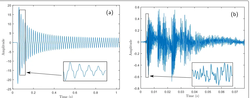
meth-ods are Prony’s [19], Pisarenko’s [20], matrix pencil [21], Estimation of Signal Parameters via Rotational Invariance Techniques (ESPRIT) [22], and MUltiple SIgnal Classifi-cation (MUSIC) [23]. Despite its success, the SDS model is inadequate for turn-on transient current signals. In fact, a lot of turn-on transient current signals are charac-terized by a quasi-stationary harmonic content (Fig.1a) whereas the SDS model is best suited for modeling van-ishing non-stationary content (Fig. 1b) because having different damping factors for each frequency produces a signal with non-stationary frequency content. Moreover, the turn-on transient current decays to a steady state that is different from the steady state preceding the turn-on

Fig. 1Two examples of transients.aA (turn-on) transient of an electrical signal (drill) for which the superimposed damped sinusoids (SDS) model is inadequate, andba transient of an audio signal (castanets) for which the SDS model is adequate. Note the non-stationary content ofband the quasi-stationary content ofa

of the appliance, whereas in the SDS the transient model starts from one steady state and decays to the same one afterwards. The electrical current “turn-on" transient is the current that appears with the switching-on of an elec-trical appliance. This corresponds to a transition from one steady state to another. For example, if we consider a single appliance on the network, then the first steady state is the state of no consumption, the second steady state is the state of steady consumption, and the tran-sient is the part in between. Note that the trantran-sient we are interested in modeling is the one related to the electri-cal consumption. This transient is different from the very high frequency transient (appearing as a short pulse pre-ceding the turn-on transient) generated by the switching devices because of the closure of the circuit [24]. Turn-on transients are appliance-dependent and last usually from few power system cycles to few seconds. A turn-on tran-sient is typically characterized by a high current amplitude (surge) at the beginning of consumption followed by a decrease (or damping) in the amplitude of the consumed energy until reaching a stable state (Fig.1a).

In this paper, we propose a new model for turn-on transient current signals along with an efficient algorithm for the parameter estimation. The parameters are used to characterize electrical appliances and are shown to be useful for appliance classification. Several objectives are targeted in this paper including:

• Derivation of an efficient estimation algorithm for the model parameters.

• Assessment of the estimation performance via the computation of the Cramér-Rao bound (CRB).

• Validation of the proposed model on real transient signals and the evaluation of the modeling error when using the developed estimation algorithm.

• Exploitation of the model parameters for appliance characterization and assessment of their usefulness as relevant features for a classification task example.

• As a by-product, we also developed a full

experimental setup (with a dedicated transient signal acquisition device) to build our dataset of real transient signals corresponding to different electrical appliances. This dataset is used for our model validation as well as for the performance assessment of the proposed appliance identification method.

The rest of the paper is organized as follows: Section2.1

describes the proposed data model, Section 2.2 details

the proposed parameter estimation algorithm, Section3

gives the derivation of the parameters’ CRBs, Section4.1 gives the assessment of the proposed model and algo-rithm on simulated and real data, Section4.2shows the usefulness of the model parameters through an appliance classification example, and finally, Section5concludes the paper.

2 Methods 2.1 Data modeling

The shape of the turn-on transient and the related amplitudes vary from one electrical appliance to another. To take into account these variations, we propose to model the noiseless electrical current turn-on transient s(t)as the product of two signals

s(t)=e(t)ss(t), ∀t∈[ 0,+∞) (1)

wheree(t)represents an amplitude modulation (envelope) andss(t)is a sum ofdsinusoids given as follows tudes, phases, and frequencies, respectively. The number

d of sinusoids (current harmonics) is assumed known

(typically d = 5 harmonics is enough to represent the

sinusoidal signal ss(t)) and the frequencies satisfy fi = (2i−1)f0,i=1,. . .,dwheref0≈50 Hz. Indeed, because of the half-wave symmetry found in electrical signals (i.e., for a periodic signalg(t)of periodP, a half-wave symme-try is characterized byg(t+P/2) = −g(t)), the sinusoid frequenciesfiare odd-order harmonics of the fundamen-tal frequency. Note that the nominal value (50 Hz) of the network fundamental frequency is a priori known, but due to its fluctuations around this value over time (i.e., f0 = 50+δf), we have observed that for a correct mod-eling,f0should be considered as unknown and hence one needs to re-estimate the fundamental frequency value for each transient signal1.

The envelopee(t)is chosen of the formeu(t)+1 such that eu(t) _{−−−−→}

t→+∞ 0. This exponential function was chosen for

its usefulness in describing damped phenomena. A classi-cal damped model is such thatu(t) = −αtwithα > 0. For our model, we propose to extend this classical model in order to adapt it to real current signals. Specifically, we propose to modelu(t)as a polynomial function allowing more flexibility in describing the amplitude modulation of real signals thatpTt is a polynomial of degreenallowing the model adaptation to the real signal variations2_{. The polynomial} is such thatpTt −→

t→+∞−∞leading toe(t)t→+∞−→ 1 (verified

ifpn<0).

1_{The European norm “EN 50160” [25] fixes the acceptable variation ranges for}

δf0. For the synchronous grid of Continental Europe—the largest synchronous (same frequency) grid in the world linking most of Europe’s countries and some countries of north Africa—these ranges are±1% off0

(δf0=[−0.5,+0.5]Hz) 99.5% of a year and−6%/+4%off0 (δf0=[−3,+2]Hz) 100% of the time. The latter range is made large to account for occasional high variations.

2_{Based on our real data measurements, we have observed that a polynomial} ordern=3is sufficient to model properly the considered transient signals.

We assume that the measured current signalx(t)is cor-rupted by an additive white Gaussian noise (AWGN)w(t) with zero mean and varianceσ2

x(t)=s(t)+w(t), ∀t∈R. (4)

The passage from continuous to discrete-time notation is done using tk = kTs, whereTs = 1/Fs is the sampling period andk∈ Z. This notation is used in the remainder of the paper.

2.2 Parameter estimation algorithm

The proposed parameter estimation algorithm proceeds in two steps:

• Estimation of the fundamental frequencyf0.

• Estimation of the other signal parameters using the a priori estimated frequencyfˆ0.

2.2.1 Fundamental frequency estimation

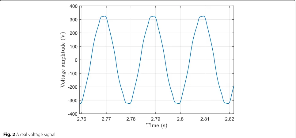
We assume that the fundamental frequency is unknown but quasi-constant over the transient duration, typically less than 5 s, and we propose to estimate it using the volt-age signal, which is almost perfectly sinusoidal (Fig.2). Indeed, the stability of f0 (i.e., its rate of change) is an important issue that was discussed in depth in the lit-erature. This can be seen from the plot in Fig. 3

(bor-rowed from http://wwwhome.cs.utwente.nl/~ptdeboer/

misc/mains.html) which represents the “Allan deviation”

of f0 for a measurement over a period of 69 days. As

explained in this reference, if the Allan deviation at an averaging duration of 10 s is 10−4, it means that if one measures the frequency during 10 s and once more during the next 10 s, these measurements will differ on average by 0.01%. Based on this, we consider the frequency variation over our 5-s measurement period as negligible. Hence, the fundamental frequency estimation problem turns into the classical problem of estimating the frequency of a mono-tone signal in noise. It is known that the CRB of the frequency parameter of a monotone signal decreases with a rate of 1/N3_[26]

var(fˆ0)≥

12

(2π)2_ηN(N2₋₁₎, (5)

where η is the signal-to-noise ratio (SNR) and N the

number of signal samples. This allows for highly precise frequency estimates. Practically, we use the algorithm

pro-posed by Aboutanios and Mulgrew [27] which is shown

to provide a precise frequency estimate reaching the CRB. Indeed, the voltage signal is modeled here as a pure

sinu-soid of frequency f0 corrupted by an AWGN. In such

Fig. 2A real voltage signal

In the second step (next section), we estimate the remaining parameters using the frequencyfˆ0.

2.2.2 Transient current estimation (TCE) algorithm

Given the estimated frequencyˆf0, the second step of our estimation algorithm operates in two phases: (i) initializa-tion and (ii) parameter estimainitializa-tion.

The initialization phase provides initial estimates of the parameterspj,ai, andφi (j = 0,. . .,nandi = 1,. . .,d) to be used in the parameter estimation phase, during which these estimates will be refined. This two-phase

structure of the algorithm is motivated by the difficulty and high computational cost of the nonlinear maximum-likelihood-based estimation criterion (see (15)). In such a case, we usually seek a good initial estimate and then refine it in order to alleviate the ill-convergence and high computational cost of the problem.

Note that the algorithm needs some pre-specified

values for n, d, and fi and also needs a pre-defined

steady state portion used in the initialization step for

the estimation of the amplitudes ai and phases φi of

the sinusoids. Hereafter, we start by discussing these

“pre-specified quantities,” then we proceed to detailing the algorithm.

Pre-specified quantities These quantities are fi(i = 1,. . .,d),n,d,tss1, and tss2 (“ss” stands for steady state). As mentioned in Section2.1, fi are odd-order harmon-ics off0. Taking into account the estimated fundamental frequencyfˆ0, the sinusoids’ frequencies are given byfi = (2i−1)fˆ0. The rest of the parameters are chosen in an

ad hoc way. The polynomial degreenand the number of

sinusoidsdwere chosen based on experimental observa-tions made on the real data we used. The chosen values

weren = 3 andd = 5 (see the discussion of assumption

A3in Section4.1.2).

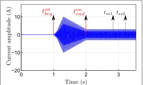
Quantities tss1 and tss2 define the time instants that delimit a portion, notedxss(tk), of the steady state of the current signal (Fig.4). This portion is used in the initial-ization phase for the estimation of the amplitudes and phases. On this steady state portion, tk ∈[tss1,tss2], we can writex(tk) = xss(tk) = ss(tk)+w(tk)wheress(tk)is the sum of sinusoids signal (2); we neglect the envelope influence by assuminge(t)=1 on this portion.

We definetss1andtss2using the High Accuracy NILM Detector (HAND) algorithm [28] found in the literature. Applying HAND on a turn-on transient signal provides the time-instantston_begandton_enddefining the beginning and end of the turn-on transition (Fig.4). Practically, we define tss1a few (typically ten) time cycles aftert_endon andtss2such that the duration ofxss(tk)is 25 time-cycles (i.e., half a sec-ond, sufficient to get good initial estimates of amplitudes and phases).

Initialization phase

1. Estimation ofss(tk): Using the least squares (LS) criterion, parametersaiandφiare estimated using

Fig. 4Output of the High Accuracy NILM Detector (HAND) when applied to a simulated single-appliance signal. HAND outputs the time-instants:ton_begandton_end. Blue: current signal.tss1andtss2define the steady state portion (25 time-cycles long) used for the estimation

(tk∈[tss1,tss2])

Writing (6) in vector form gives

xss=Mc+w, (7)

The LS criterion, used to find an estimate forc, aims to minimize the square of the Euclidean norm ( · 2)

of the difference between the measured signal and the data model, i.e.,

In that case, the solutioncˆis given by

rCˆlcˆ=M+xss, (10)

whereM+=(MTM)−1MT is the (Moore-Penrose) pseudo-inverse ofM. We extract fromˆctwo vectors

ˆ

where andare the element-wise product and division operators, respectively.

2. Estimation ofe(t_k):

region” class of algorithms [31]. This algorithm allows constraints to be imposed on the values of the parameter estimates enabling us to satisfy our constraints (ai≥0,φi∈[−π,π]andpn<0). Having the estimatesaˆandφˆ obtained from the previous step and the (overall) measured signal

x=[x(t0),. . .,x(tN−1)]T, we estimate an initial value

Moreover,t0is practically chosen as the time-instant

corresponding to the maximum current amplitude; that way, we model the damped part of the turn-on transient starting from the maximum amplitude. In the end of this phase, we obtain the initial estimated

parameter vectorθˆ0=

ˆ

pT,aˆT,φˆTT.

Parameter estimation phase As the estimation ofaiand φiis done using only a portion of the total measured sig-nalx(tk), the aim of this parameter estimation phase is to improve the estimation of all the parameters by consid-ering all the samples of x(tk). We use for this the same TRR algorithm considered for the estimation ofe(tk) by taking as initial value the result of the estimation phase

ˆ

θ0. The unknown, to be estimated this time, is the global parameter vectorθ =pT,aT,φTTestimated as

The TCE algorithm is summarized in Algorithm1.

3 Cramér-Rao bounds of the model parameters The Cramér-Rao bound (CRB) provides a lower bound on the variance of any unbiased estimator. We show in Section4.1.1that this unbiasedness condition is approxi-mately verified (at least for moderate and high SNRs) for our estimated parameters, and hence, we can use the CRB to assess the performance of our estimation.

Evaluating the performance of the estimation consists of comparing the estimated parameters’ variances with their CRB. Taking into account the dependence ofs(tk)on the parameter vector θ andN samples of x(tk), (4) can be written using vector notation as

x=s(θ)+w, (15)

wherexis normally distributed with meanμ(θ)=s(θ)= [s(t0,θ),. . .,s(tN−1,θ)]Tand a covariance matrixC(θ)= C=σ2I.

Algorithm 1: Transient Current Estimation (TCE) algorithm

using the least squares (LS) criterion where

ˆ

using the TRR algorithm [29,30] initialized by

p0=0.Movis the matrixM(8) with

The CRB is defined as the inverse of the Fisher infor-mation matrix (FIM). If we assumeθ = pT,aT,φTT = [θ1,. . .,θK]T,K=n+1+2d(the noise power is assumed known here) andx=[x(t0),. . .,x(tN−1)]T∈RN, then for the general Gaussian case wherex ∼ N(μ(θ),C(θ)), the FIM is given elementwise by [26]

The symbol [·]i denotes element of indexiof the corre-sponding vector, [·]_ij denotes the element of index ij of the corresponding matrix, and tr [·] denotes the trace operator.

For our model whereμ(θ) = s(θ) andC(θ) = σ2I

(covariance matrix independent ofθ), the (elementwise) FIM becomes

Taking into account (17) and the structure ofθ, the FIM can be written using matrix notation in the form of a nineblock matrix representing the partial derivatives with respect to the elements ofθ as

F(θ)= 1

Since this matrix is symmetric (because of the symmetry of the second order partial derivatives), we only have to compute the following terms to find all the elements of the matrix:∂_∂s_pT After straightforward derivations, we get

∂sT equal toF−1(θ)obtained after inserting expressions (19) in (18) and invertingF(θ).

In the previous CRB derivation, we assumed the noise varianceσ2_{known so thatK =n+1+2d. If we assume}

that σ2 _{is also an unknown parameter to be estimated}

such thatθ = pT,aT,φT,σ2T, then the FIMFθis

equal to the FIMF(θ)augmented with one row and one

column corresponding to partial derivatives with respect toσ2. Using (16), we get

The CRB is then given by

CRB(θ)=F−1θ=

This indicates that it is sufficient to independently com-puteF−1(θ)and 2_Nσ4 to findF−1θ. It also means that the existence or lack of information about σ2 does not affect the performance bound (CRB) of the other desired parameters.

4 Results and discussion

4.1 Estimation performance assessment

4.1.1 Assessment on simulated data

In this section, we present the results of the estimation performance evaluation on simulated data. Hereafter, we present (i) the simulated signal and its parameters, (ii) the bias of the estimated parameters, (iii) the estimated parameters variance and its comparison to the CRB, (iv) the CRB variation with respect to the sampling frequency, and (v) the convergence of the TCE algorithm.

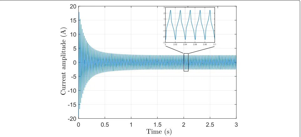
Simulated signal and its parameters Taking the consid-ered setup (n = 3 andd = 5) in this section, we end up with 14 parameters for the simulated signal. So, with such large number of degrees of freedom, we decided to choose the set of parameters such that the simulated signal will resemble as much as possible real signals, and without a priori knowledge on what parameter values are appropri-ate, we decided to tweak the model parameters and choose the ones that gave a simulated signal “resembling” (sim-ilar waveform) typical real current waveforms from our dataset. The noiseless signal model is

s(tk)=e(tk)ss(tk)=

f0 = 50 Hz. The chosen model parameter values are

Fs=30 kHz: sampling frequency

t0=0 s,tN−1=3 s: specify signal duration n=3: polynomial degree

d=5: number of harmonics

p=[ 1.9,−9, 8.5,−4]T

a=[ 1.8, 0.5, 0.2, 0.1, 0.05]T φ=[−3, 3, 2.5, 1.5, 1]T

The polynomial degree is chosen relatively small (we found thatn = 3 is sufficient to characterize the tested signals, and hence, this value will be used in the remainder of the paper). The previous transient signal is then cor-rupted by an additive white Gaussian noise of zero mean and varianceσ2(varied such that the signal-to-noise ratio

(SNR)= 1/N N−1

k=0 s(tk)2

σ2 varies in the range [ 0−50] dB).

The obtained simulated signal is shown in Fig.5.

Bias of the estimated parameters As mentioned before, the CRB applies for unbiased estimators. Our maximum likelihood estimation method based on criterion (14) is known to be asymptotically, i.e., for high SNR, unbiased [26]. Here, we evaluate our estimator bias numerically using (1000) Monte-Carlo runs.

Figure 6 gives the bias computed for the parameters

estimated using the proposed algorithm versus the signal-to-noise ratio (SNR). We can see that all estimated param-eters have negligible bias for SNR values greater than or equal to 30 dB. Between 10 dB and 30 dB, the estimated parameters have very small biases, and below 10 dB, we start getting some bias, nonetheless with values that are still small compared to the true parameter values.

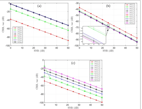
Estimated parameters’ variance and its comparison to the CRB Similarly to the bias computation, the variance is also computed numerically. Figure7shows the differ-ent parameter variances compared with their respective CRBs. We note that all the parameter variances coincide with their respective CRBs almost perfectly. Hence, our estimation is efficient (unbiased and the variance reaches the CRB).

CRB variation with respect to the sampling frequency

Due to the transient behavior of the observed phenomena, a good choice for the sampling frequencyFsof measure-ments is mandatory. We seek a sufficiently high sampling frequency to catch the transient behavior but not too high to avoid heavy computational load. The CRB allows us to evaluate the impact of the sampling frequency on the parameter variance lower bounds and therefore decide on the desired performance taking into account computa-tional complexity.

Figure8gives the variation of the parameters’ CRB as a function ofFs(1 to 100 kHz) on a logarithmic scale. The results show that an increase inFsresults in a better esti-mation performance (linearly decreasing variance w.r.t. to the sample size) for all the parameters. This is expected, since a higherFsmeans more data samples (on a fixed time period) and hence better performance. When consider-ing real signals, however, this is not necessarily true. The white noise (independence) assumption initially verified for relatively lowFs (still high frequency though) might not be verified in practice for higher frequency values. At higher frequencies, the data samples become closer and might become correlated, when the time duration between two samples is too small to assume indepen-dence. In that case, the computed CRB assuming a white noise can no longer be used to evaluate the estimation performance.

Practically, finding the adequate sampling frequency is not easy since it depends on different parameters: transient waveforms of interest and their frequency con-tents, computational complexity, desired performance,

Fig. 6Bias of the different parameters estimated using the TCE algorithm.aBias ofpˆ,p₌[ 1.9,₋9, 8.5,₋4]T_{.bBias ofaˆ,a=[ 1.8, 0.5, 0.2, 0.1, 0.05]}T_. cBias of_φˆ,_φ=[₋3, 3, 2.5, 1.5, 1]T_{. We used 1000 Monte-Carlo runs}

etc. According to our experiments, and for the study of turn-on transient signals, a sampling frequency at least equal to 5 kHz is recommended (captures around 50 har-monics) whereas going beyond 100 kHz starts generating heavy data processing. A sampling frequency of 30 kHz seems to be a good compromise, since it captures around 300 harmonics and is less computationally heavy. Hence, our choice wasFs=30 kHz for simulations.

Convergence of the TCE algorithm Since the TCE algo-rithm uses an optimization algoalgo-rithm in both its estima-tion and refinement phases, it is important to check its convergence, especially if there is a need for real-time processing. Hereafter, we check the convergence of the nonlinear optimization algorithm, trust-region-reflective (TRR), for both phases.

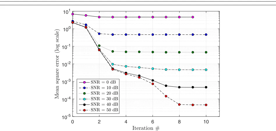
Figure 9 gives, for different SNR values, the

mean-square-error (MSE) as a function of the number of iter-ations in the estimation phase of the TCE algorithm.

Independently of the SNR, the algorithm converges after ten iterations. The convergence of the TRR algorithm in the refinement phase is even faster. Indeed, the initializa-tion point being better defined, it converges at most after three iterations.

4.1.2 Assessment on real data

Real data considerations Until now, we have implicitly assumed, for simulated data, some simplifying assump-tions to test the parameter estimation independently of the performance of other blocs that may condition the estimation. These assumptions are as follows: (A1) a well-defined portion of the steady state, (A2) transient starting

from a maximum, and (A3) known polynomial degree

n and number of harmonics d. In real situations,

Fig. 7Comparison of the CRB and estimated parameters’ variance. Represented is the CRB vs. variance forp(a),a(b), and_φ(c). The CRB curves are represented using dashed lines and the variance curves using solid lines. We used 1000 Monte-Carlo runs

accuracy); (ii) physically, there will always be a latency in the appliance response before the current signal reaches its maximum amplitude; and (iii) the polynomial degree as well as the harmonic numbers are only chosen param-eters used to trade-off between complexity and modeling efficiency.

The easiest assumption to get around in a real situation

isA2since we only need to detect the signal maximum

amplitude and model the damped part, starting from this maximum (so the portion of transient signal preceding the peak value will be disregarded). For assumptionA1, we use the HAND detector [28] built specifically to allow high accuracy detection of turn-on transients. ForA3, we relied on our dataset of real life signals to get our ad hoc

choice of the “effective” polynomial degree n = 3 and

“effective” number of harmonics d = 5 that have been

experimentally shown to be suitable for a good model-ing of the considered transient signals. As an example,

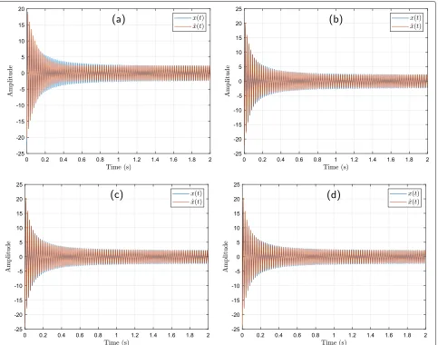
Fig. 10 shows different plots comparing the real signal x(t)to its estimatexˆ(t)for different values of the

polyno-mial degreen(1, 3, 5 and 7). We note the improvement

of the root-mean-square error (RMSE) betweenn = 1

and n = 3, hence a better estimation using n = 3,

and a slight improvement of the RMSE betweenn = 3,

n = 5, and n = 7. We considern = 3 to be a good

trade-off between model complexity and the estimation performance (less than 10% of relative RMSE difference,

e.g., betweenn = 3 andn = 5, we have a relative RMSE

difference of 0.2473_0.2473−0.2433 ≈1.6%).

Fig. 8CRB of the model parameters as a function of the sampling frequencyFs(from 1 kHz to 100 kHz) at an SNR of 25 dB. Represented is the CRB of p(a),a(b), and_φ(c)

Fig. 9Mean square error (MSE)1 N

N−1

Fig. 10Comparison between real,x(t), and estimated,ˆx(t), transient current signals of a drill using different polynomial degreesn. The pairs (polynomial degree, root-mean-square errors) (i.e., (n, RMSE)) for the different panels are(n=1, 0.2962)(a),(n=3, 0.2473)(b),(n=5, 0.2433)(c), and(n=7, 0.2428)(d)

also tried to improve the estimate of f0 by jointly esti-mating it when (i) estiesti-mating pˆ (13), (ii) when refining the estimation of all parameters (14), and (iii) in both (i) and (ii). This, however, did not improve the results, indi-cating that the proposed approach already leads to near optimal values (due in part to the highly precise estimate off0 obtained using [27]). As an example, we have con-ducted the joint estimations described above considering the real signal used in Fig.10withn=3 that gave initially RMSE = 0.2473. The newly obtained results, in terms of RMSE, were 0.2473, 0.2479, and 0.2479, respectively for (i), (ii), and (iii). The joint estimation off0 was not con-sidered further as it would generate more computational load without performance gain.

Estimation with TCE on a real signal of the COOLL dataset The real signal is taken from a turn-on tran-sient dataset we built especially for trantran-sients analysis.

The dataset is called Controlled On/Off Loads Library

(COOLL) [32] and is freely available on the internet

(https://coolldataset.github.io/). Since the measurement system [33] (Fig.11) used to collect the dataset’s signals allows the control over the turn-on/off, we know exactly the turn-on/off time instants and assumptionsA1andA2

hold then true. Moreover, we consider the signal starting from its maximum in order to verifyA3.

The COOLL dataset signals (Table 1) are sampled at

Fs = 100 kHz3. The dataset consists of turn-on transient current and voltage signals of 12 different electrical appli-ances and each appliance has 20 signal examples. Figure12 shows a typical histogram of the noise on a measured cur-rent signal taken from its pre-turn-on part (noise only).

3_{After measurements were done we found thatF}

s=30kHz would have been

Fig. 11Photograph of the measurement system

This shows that the noise distribution for the COOLL cur-rent signals is Gaussian with zero mean and a standard deviation of 2.2 mA (equivalent to an approximate power consumption of 0.5 W).

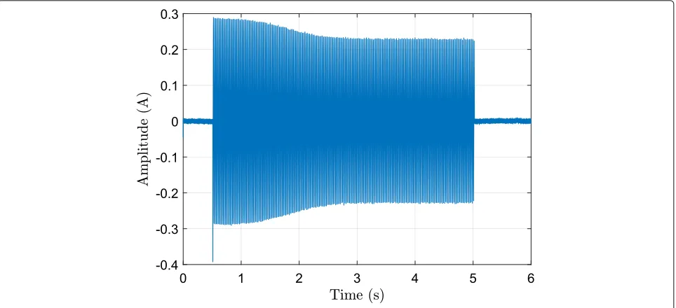
Next, we provide an illustrative example corresponding to a test signal of a fan (Fig.13). The total duration of the measurement is 6 s with a 0.5 s of pre-turn-on. The esti-mation results of TCE on the fan signal (Fig.13) are as follows:

Table 1COOLL dataset summary

N° Appliance type No. of appliances No. of current signals (20 per appliance)

1 Drill 6 120

2 Fan 2 40

3 Grinder 2 40

4 Hair dryer 4 80

5 Hedge trimmer 3 60

6 Lamp 4 80

7 Paint stripper 1 20

8 Planer 1 20

9 Routera _{1 20}

10 Sander 3 60

11 Saw 8 160

12 Vacuum cleaner 7 140

Total 42 840

a_{This is an electrical router for woodworking not a network router}

lpˆ=

Fig. 13Turn-on transient current of a fan from the COOLL dataset

where RMSE is the root-mean-square-error. The above estimation results indicate little information on the esti-mation quality, especially that we are applying the algo-rithm on a real signal. Nonetheless, the RMSE gives an idea about the estimation quality but is still without much meaning if not considered relative to some refer-ence value. Here, we propose to compare it to the average maximum value of the steady state amplitude (around 0.2 A). We get a relative RMSE of 3.6%. Note that we got an average relative RMSE of around 8% for the whole dataset, which is acceptable considering the variability of real signals.

Figure 14 allows to get a visual feel for the

esti-mation quality. Figure 14a and b show a good fit

between the reconstructed signal and the original zone.

4.2 Classification of cOOLL dataset’s appliances using the model parameters

Here, we propose to classify the appliances of the COOLL dataset using the model parameters. We use the clas-sical supervised k-nearest neighbors algorithm (k-NN) [34, Chap. 13], which proceeds by taking the test exam-ple (here the vector of parameters representing the test signal) and classifying it according to a majority vote of the k-nearest examples (of the training dataset). We used the Euclidean distance as a distance metric. We assess

the result using K-fold cross-validation with K = 10.

This validation works by first partitioning the dataset to K equal partitions (in our case each partition contains 84 example), then take one partition for testing and keep

the other nine partitions for training, and we assess the performance using for example the classification accuracy (CA). This process is repeatedKtimes, taking at each time a different partition for testing and the remaining nine for training. The final result is the average of theKaccuracy results.

Note that the estimated values of the phase parame-ters φi are too random to be considered as features for the classification and, hence, are discarded hereafter. We apply the k-NN on the data using the estimatedpˆj,j = 0,. . ., 3 andaˆi,i=1,. . ., 5. The results are presented as a confusion matrix (Fig.15).

Fig. 14Turn-on transient current of a fan from the COOLL dataset (in blue) with the reconstructed signal (in red) generated using the estimated parameters with the TCE algorithm.aCurrent signals,bzoom on the interval [ 0.50₋0.60] s, andczoom on the interval [ 3.50₋3.60] s

Fig. 16Four examples of turn-on transient signals.aDrill,bhair drayer,cpaint stripper, anddfluorescent lamp. Note the different envelope shapes for the different appliances, which gives different minimum radii of curvature

examples are correctly classified among 121 classified as a drill (column sum)).

We obtain a CA of 92.4%. Although the CA is higher than 92%, we expect a less variable characteristic feature capturing the envelope shape to be more relevant for the classification. In fact, the pˆj are sensitive to the chosen origin of time (except the last parameter pˆn) and their estimated values are less stable due to the difficulty of pre-cisely defining the origin of time for transient signals. To remedy this, we need to construct a new feature that is independent of the time origin and that still is characteris-tic of the envelope shape. We propose to use theminimum radius of curvature of the estimated envelope signalˆe(t) constructed using thepˆjparameters. For a functionf(t), the radius of curvature at pointt0is defined as [35]

R(t0)=

(1+f(t0)2)3/2 f(t0)

(22)

wheref(t0)andf(t0)are the first and second derivatives of f(t) at pointt0, respectively. Practically, we compute this value for each sample point of eˆ(tk) and take the

minimum value Rmin. This minimum value is inversely

proportional to the maximum curvature, which is a dis-tinctive feature of the turn-on transient signals as can be seen in Fig.16.

Fig. 17Stability of the minimum radius of curvature versus various values of the grid phase (action delay) for two appliances (a drill and a vacuum cleaner). Action delay is the delay w.r.t. the (positive-to-negative) zero-crossing of the voltage signal before switching-on an appliance, e.g., an action delay of 4 ms means that the appliance is switched-on after 4 ms of voltage zero-crossing

The classification results usingRminandaˆi are shown in Fig. 18. Compared to the previous result, we obtain

an improvement of 5.6%, with a CA of 98.0%. Another

performance metric used often in assessing classification performance is the F1 score defined as 2precision_precision×₊recall_recall. This metric can be computed for each appliance and gives a single number assessing the performance, which is espe-cially helpful when comparing different classifiers or, as is the case here, the result of two different sets of features.

The F1 score results for our classification are given in

Table 2. These results show an improvement in the F1

score for almost all the appliances when using the set of features{Rmin,aˆi}compared to the set of features{ˆpj,aˆi}.

5 Conclusion

We proposed in this paper a new mathematical represen-tation suitable for modeling turn-on transient current sig-nals and proposed an algorithm for the model parameter estimation. The efficiency of the algorithm is assessed

Fig. 19Turn-on transient current of a microwave

theoretically via benchmarking its estimation error vari-ances with respect to the CRB derived in Section3of this paper. Later on, the proposed parametric model is vali-dated using real data from the COOLL dataset that we developed specifically for this research work. A “good” fit-ting between the proposed signal model and the real-life signals has been observed with, in particular, an average relative mean-square-error of about 8%. Note also that our experimental tests showed the need for estimating the fundamental frequency due to its deviation from the nominal value (i.e., 50 Hz). A classification method using the model parameters has been proposed. The obtained

Table 2Comparative F1 scores of the different COOLL appliances for the classification result using the two sets of features{ˆpj,aˆi}and{Rmin,aˆi},j=0,. . ., 3, andi=1,. . ., 5

results show the usefulness of the transient signal param-eters as relevant features for the characterization of elec-trical appliances with a correct classification accuracy of 98% in the considered context.

The proposed model is valid for a lot of electrical appliances that show a single-phase behavior during the turn-on such as incandescent light bulbs, compact fluo-rescent lamps, heaters, vacuum cleaners, and hairdryers. However, some electrical appliances may have a turn-on transient current signal cturn-onsisting of different phases each with a distinct signal content (harmonics with dif-ferent amplitudes and phases) and a distinct envelope shape corresponding to the different regimes that the appliance goes through during turn-on. For instance, the

microwave turn-on transient shown in Fig. 19 has two

phases (some microwaves may have more than two) each with its specific characteristics. As a perspective work, one can consider using our model to characterize each phase independently (as a single-phase appliance) and then devise some rule to identify the corresponding multi-phase appliance (e.g., considering the occurrence of the different phases in a time series).

Abbreviations

CA: Classification accuracy; COOLL: Controlled On/Off Loads Library; CP: Classified as positives; CRB: Cramér-Rao bound; ESPRIT: Estimation of Signal Parameters via Rotational Invariance Techniques; FIM: Fisher information matrix; HAND: High Accuracy NILM Detector; k-NN: k-nearest neighbors; LM: Levenberg-Marquardt; LS: Least squares; MSE: Mean-square-error; MUSIC: Multiple Signal Classification; NILM: Non-intrusive load monitoring; RMSE: Root-mean-square-error; RP: Relevant positives; SDS: Superimposed damped sinusoids; SNR: Signal-to-noise ratio; TCE: Transient current estimation; TP: True positives; TRR: Trust-region-reflective

Acknowledgements Not applicable.

Authors’ contributions

MNM, PR, KAM, and GL conceived and designed the experiments, analyzed the data, and interpreted the results. MNM performed the experiments and wrote the manuscript. MNM, PR, and KAM contributed in developing the model and parameter estimation algorithm. JCLB and YR provided their expertise for the power grid aspects of the experiments. All authors read and approved the final manuscript.

Funding

This current study was supported in part by the Région Centre-Val de Loire (France) through the project MDE-MAC3 (Contract no 2012 00073640).

Availability of data and materials

The dataset created and used during the current study is freely available athttps://coolldataset.github.io/.

Competing interests

The authors declare that they have no competing interests.

Author details

1_{PRISME Laboratory, University of Orléans, 12 rue de Blois, 45067 Orléans,} France.2_{GREMAN Laboratory, UMR 7347 CNRS–University of Tours, 20 avenue} Monge, 37200 Tours, France.

References

1. C. A. García, A. Otero, X. Vila, D. G. Márquez, A new algorithm for wavelet-based heart rate variability analysis. Biomed. Signal Process. Control.8(6), 542–550 (2013).https://doi.org/10.1016/j.bspc.2013.05.006 2. X. Chen, H. Wen, Q. Li, T. Wang, S. Chen, Y.-P. Zheng, Z. Zhang, Identifying

transient patterns of in vivo muscle behaviors during isometric contraction by local polynomial regression. Biomed. Signal Process. Control.24, 93–102 (2016).https://doi.org/10.1016/j.bspc.2015.09.009 3. T. P. Exarchos, A. T. Tzallas, D. I. Fotiadis, S. Konitsiotis, S. Giannopoulos, EEG transient event detection and classification using association rules. IEEE Trans. Inf. Technol. Biomed.10(3), 451–457 (2006).https://doi.org/10. 1109/TITB.2006.872067

4. A. Belsak, J. Flasker, Adaptive wavelet transform method to identify cracks in gears. EURASIP J. Adv. Signal Proc.2010(1), 879875 (2010).https://doi. org/10.1155/2010/879875

5. C. Capilla, Application of the Haar wavelet transform to detect

microseismic signal arrivals. J. Appl. Geophys.59(1), 36–46 (2006).https:// doi.org/10.1016/j.jappgeo.2005.07.005

6. X. Li, Z. Li, E. Wang, J. Feng, L. Chen, N. Li, X. Kong, Extraction of microseismic waveforms characteristics prior to rock burst using hilbert–huang transform. Measurement.91, 101–113 (2016).https://doi. org/10.1016/j.measurement.2016.05.045

7. J. Seymour, T. Horsley, The seven types of power problems. White paper. 18, 1–21 (2005)

8. M. H. J. Bollen, E. Styvaktakis, I. Y.-H. Gu, Categorization and analysis of power system transients. IEEE Trans Power Deliv.20(3), 2298–2306 (2005). https://doi.org/10.1109/TPWRD.2004.843386

9. S. Wang, Z. K. Zhu, Y. He, W. Huang, Adaptive parameter identification based on Morlet wavelet and application in gearbox fault feature detection. EURASIP J. Adv. Signal Process.2010(1), 842879 (2010).https:// doi.org/10.1155/2010/842879

10. W. Jiao, S. Qian, Y. Chang, S. Yang, Research on vibration response of a multi-faulted rotor system using LMD-based time-frequency

representation. EURASIP J. Adv. Signal Process.2012(1), 73 (2012).https:// doi.org/10.1186/1687-6180-2012-73

11. S. B. Leeb, S. R. Shaw, J. L. Kirtley Jr, Transient event detection in spectral envelope estimates for nonintrusive load monitoring. Power Deliv. IEEE Trans.10(3), 1200–1210 (1995)

12. C. Laughman, K. Lee, R. Cox, S. Shaw, S. Leeb, L. Norford, P. Armstrong, Power signature analysis. Power Energy Mag. IEEE.1(2), 56–63 (2003) 13. H.-H. Chang, H.-T. Yang, Applying a non-intrusive energy-management

system to economic dispatch for a cogeneration system and power utility. Appl. Energy.86(11), 2335–2343 (2009)

14. R. Kumaresan, D. Tufts, Estimating the parameters of exponentially damped sinusoids and pole-zero modeling in noise. IEEE Trans. Acoust. Speech. Signal Process.30(6), 833–840 (1982)

15. L. Lovisolo, M. P. Tcheou, E. A. B. da Silva, M. A. M. Rodrigues, P. S. R. Diniz, Modeling of electric disturbance signals using damped sinusoids via atomic decompositions and its applications. EURASIP J. Adv. Signal Process.2007(1), 029507 (2007).https://doi.org/10.1155/2007/29507 16. R. Boyer, K. Abed-Meraim, Audio modeling based on delayed sinusoids.

IEEE Trans. Speech Audio Process.12(2), 110–120 (2004).https://doi.org/ 10.1109/TSA.2003.819953

17. D. V. Rubtsov, J. L. Griffin, Time-domain Bayesian detection and estimation of noisy damped sinusoidal signals applied to NMR spectroscopy. J Magn. Reson.188(2), 367–379 (2007).https://doi.org/10.1016/j.jmr.2007.08.008 18. M. A. Al-Radhawi, K. Abed-Meraim, Parameter estimation of

superimposed damped sinusoids using exponential windows. Signal Process.100, 16–22 (2014).https://doi.org/10.1016/j.sigpro.2013.12.025 19. R. Prony, Essai expérimental et analytique : sur les lois de la dilatabilité des

fluides élastiques et sur celles de la force expansive de la vapeur de l’eau et de la vapeur de l’alkool, à différentes températures. J. de l’École Polytechnique Floréal et Plairial.1(22), 24–76 (1795)

20. V. F. Pisarenko, The retrieval of harmonics from a covariance function. Geophys. J. Int.33(3), 347–366 (1973)

21. Y. Hua, T. K. Sarkar, Matrix pencil method for estimating parameters of exponentially damped/undamped sinusoids in noise. Acoust. Speech. Signal Process. IEEE Trans.38(5), 814–824 (1990)

22. R. Roy, T. Kailath, ESPRIT—estimation of signal parameters via rotational invariance techniques. Acoust. Speech. Signal Process. IEEE Trans.37(7), 984–995 (1989)

23. R. Schmidt, Multiple emitter location and signal parameter estimation. IEEE Trans. Antennas Propag.34(3), 276–280 (1986)

24. E. K. Howell, How switches produce electrical noise. Electromagn. Compat. IEEE Trans.EMC-21(3), 162–170 (1979)

25. CENELEC, Voltage characteristics of electricity supplied by public electricity networks. European Standard EN 50160 (2010)

26. S. M. Kay,Fundamentals of Statistical Signal Processing, Volume I: Estimation Theory. (Prentice Hall PTR, Upper Saddle River, 1993)

27. E. Aboutanios, B. Mulgrew, Iterative frequency estimation by interpolation on fourier coefficients. IEEE Trans. Signal Process.53(4), 1237–1242 (2005) 28. M. Nait Meziane, P. Ravier, G. Lamarque, J.-C. Le Bunetel, Y. Raingeaud, in

42nd IEEE International Conference on Acoustics, Speech and Signal Processing (ICASSP). High accuracy event detection for non-intrusive load monitoring (IEEE, 2017), pp. 2452–2456.https://doi.org/10.1109/ICASSP. 2017.7952597

29. T. F. Coleman, Y. Li, On the convergence of interior-reflective newton methods for nonlinear minimization subject to bounds. Math. Program. 67(1), 189–224 (1994).https://doi.org/10.1007/BF01582221

30. T. F. Coleman, Y. Li, An interior trust region approach for nonlinear minimization subject to bounds. SIAM J. Optim.6(2), 418–445 (1996). https://doi.org/10.1137/0806023

31. Y.-x. Yuan, inIciam. A review of trust region algorithms for optimization, vol. 99 (Citeseer, 2000), pp. 271–282

32. T. Picon, M. Nait Meziane, P. Ravier, G. Lamarque, C. Novello, J.-C. Le Bunetel, Y. Raingeaud, COOLL: Controlled on/off loads library, a public dataset of high-sampled electrical signals for appliance identification. arXiv preprint arXiv:1611.05803 [cs.OH] (2016)

33. M. Nait Meziane, T. Picon, P. Ravier, G. Lamarque, J.-C. Le Bunetel, Y. Raingeaud, inConference on Environment and Electrical Engineering (EEEIC), 2016 Proceedings of the 16th IEEE International. A measurement system for creating datasets of on/off-controlled electrical loads, (2016),

pp. 2579–2583

34. J. Friedman, T. Hastie, R. Tibshirani,The Elements of Statistical Learning. vol. 1. (Springer, New York, 2001)

35. J. D. Lawrence,A Catalog of Special Plane Curves. (Courier Corporation, North Chelmsford, 1972)

Publisher’s Note