Variability in MLT dynamics and species concentrations as observed by WINDII
Gordon G. Shepherd, Shengpan Zhang, and Xialong Wang
Centre for Research in Earth and Space Science, York University, Toronto, Canada (Received July 24, 1998; Revised January 8, 1999; Accepted January 8, 1999)
Airglow variability is a topic that has been studied for decades but an understanding of the role of the dynamical influence underlying this variability has only been achieved recently. The UARS dynamics instruments, HRDI (High Resolution Doppler Imager) and WINDII (WIND Imaging Interferometer) have been instrumental in providing this understanding, because they measure both winds and emission rates, and so are able to determine the coupling be-tween the two. But ground-based observations are also an essential ingredient to this understanding, which has grown through intercomparisons between dataset and models through workshops such as DYSMER. This presentation begins by describing the influence of the diurnal tide on oxygen and hydroxyl airglow emission rates, including the seasonal variation. This is followed by a description of two planetary scale disturbance phenomena, the springtime transition, and a stratospheric warming. Auroral influences are also considered. While these investigations cover a wide range of mechanisms there is an underlying thread which is that it is these large scale dynamical processes that are responsible for determining the distribution of the airglow patterns detected, and thus the distribution of concentration of atomic oxygen.
1.
Introduction
Our understanding of MLT variability has expanded rapid-ly following the launch of NASA’s Upper Atmosphere Research Satellite (UARS) as the HRDI (High Resolution Doppler Imager) and WINDII (Wind Imaging Interferome-ter) instruments have yielded a wealth of data on this subject. Because these instruments measure both the winds and the emission rates it has been possible to directly link the effects relating these quantities. At the same time, comparisons of HRDI and WINDII data with those obtained from ground-based and other measurements through workshops such as DYSMER have advanced the understanding of the commu-nity concerning the processes involved. A review of this subject is now a major topic, and what is presented here will be only a brief summary of recent developments. Airglow variability is a rich subject for exploration because there are decades of data available but we have only recently begun to obtain the benefits from this. Thus this paper begins with a brief discussion of the oxygen airglow, and why it is so important in relation to MLT dynamics. We then proceed to discuss this relationship in the context of tides and seasonal effects before going on to two topics focused on planetary scale disturbances, the “springtime transition” and strato-spheric warmings.
The satellite data presented are all from WINDII because these data are readily available to us, and because our un-derstanding has developed from these data (some ground-based data are also included illustrating their often crucial role in relation to satellite data). WINDII is a field-widened Doppler imaging Michelson interferometer (Shepherdet al.,
Copy right cThe Society of Geomagnetism and Earth, Planetary and Space Sciences (SGEPSS); The Seismological Society of Japan; The Volcanological Society of Japan; The Geodetic Society of Japan; The Japanese Society for Planetary Sciences.
1993), essentially a CCD camera that views the earth’s limb through a Michelson interferometer whose optical path dif-ference (time delay) is quasi-fixed at a value large enough to make possible the measurement of Doppler shifts as small as 5 m s−1. The field-widening refers to a configuration in which refractive materials are used in the arms of the inter-ferometer in order to make the phase vary slowly over the field of view as required for this imaging application. The interferometer modulates the incoming light so that its phase, and hence the wind, may be detected for each pixel in the image, but since it does not attenuate the light significantly the instrument is as sensitive as the CCD camera itself. The result is that WINDII can make accurate measurements of winds and emission rates from the atomic oxygen green line emission at 558 nm during night as well as in the daytime, including the determination of vertical profiles, even for very weak emission, including the hydroxyl airglow as well as the oxygen airglow. This large sensitivity is the key to many of the interpretations which have been made with these data.
2.
Airglow
The processes leading to the production of atomic oxy-gen in the upper atmosphere, through photodissociation of O2, are well described by Tohmatsu (1990). Photodissocia-tion in the Schumann-Runge continuum begins a little below 140 km, and is complete by about 90 km. The bulk of the production is above the level where the oxygen airglow is ob-served, so as has long been recognized, dynamical processes are required to bring the atomic oxygen down to where the at-mosphere is dense enough for the photochemistry to proceed. Historically the sole dynamical process has been assumed to be small scale mixing effects. However, it will be seen that the large scale dynamics observed by WINDII must play a major role; specific mechanisms involved are described by
Fig. 1. Illustrating the photodissociation of molecular oxygen, the down-ward transport of O through dynamical processes, and the formation of the green line and hydroxyl airglows.
Ward (1999). For the atomic oxygen green line airglow OI 558 nm originating from O(1S) this is a two-step process as follows (McDadeet al., 1986):
O+O+M→O∗2+M, O∗2+O→O(1S)+O2,
where M is a third body (most often N2) and O∗2is an uniden-tified state of O2, the so-called precursor of O(1S). Because the O(1S) is a direct result of the recombination of atomic oxygen, the airglow is a measure of the atomic oxygen con-centration; one can readily convert one to a knowledge of the other. Besides the atomic oxygen green line WINDII also observes emission from the Meinel bands of the hydroxyl radical (Fig. 1).
O+O2+M→O3+M,
H+O3→OH∗+O2,
where OH∗ is the excited state giving rise to the Meinel bands. Since these reactions are also controlled by atomic oxygen, observations of the hydroxyl airglow allow us to extend our understanding of the dynamical processes that transport atomic oxygen at lower altitudes than are accessi-ble from the oxygen airglow.
3.
Tidal Variations
The influence of dynamics on the airglow is readily ap-parent in those motions driven by the diurnal tide, especially
equator, where, in the evening, the tidal influence pushes the layer down, and causes it to brighten. But there is a limit to this process, as the emission becomes quenched below a certain altitude, as well as the precursor, and the supply of oxygen begins to run out. For these reasons the emission almost disappears at about midnight, but then begins to reap-pear at a higher normal altitude as dawn approaches, and a fresh supply of atomic oxygen is introduced.
These effects were simulated with the TIME-GCM model by Roble and Shepherd (1997), in which excellent agreement with the WINDII equinox data was found with the input of a strong diurnal tide at the bottom (30 km) of the model. More recently, Shepherd et al. (1998) presented WINDII and ground-based comparisons with the TIME-GCM model at mid-latitudes, for both equinox and solstice. Here, the di-urnal pattern of emission rate variation changes substantially between equinox and solstice, as a result of the changing relative contributions of the diurnal and semi-diurnal tide. This is consistent with the seasonal variations of these tides as shown by McLandresset al.(1996), with the diurnal tide having its maximum at equinox, and the semi-diurnal tide having its maximum at solstice.
(a)
(b)
(c)
Fig. 2. WINDII data for equinox, March/April 1993, for 02:00 LT, showing (a) the meridional wind in m s−1where solid and dashed contours indicate
respectively northward and southward directions, (b) the atomic oxygen green line emission rate in photons cm−3s−1, and (c) the hydroxyl volume emission rate in the same units.
McLandresset al.(1996). Thus it is to be expected that the green line and hydroxyl emissions should be out of phase. This is true at the equator but not necessarily elsewhere as the altitude of the airglow layers varies with latitude; the peak volume emission rate for the green line at 35◦S is at 94 km, while the altitude for the OH emission peak is 88 km at mid-latitudes, a difference between the two of only 6 km.
The situation changes significantly at solstice, as shown in Fig. 3. In Fig. 3(a) it can be seen that the symmetry in the meridional wind pattern that existed at equinox is not now as well defined, indicating the change resulting from the greater role of the semi-diurnal tide. This change does not affect the equatorial green line emission pattern profoundly, as the emission there still has a minimum at 5◦N, but the vol-ume emission rate has dropped from 85 photons cm−3s−1to 48, a reduction of 60%. The peak volume emission rates are also lower at the mid-latitude maxima; 163 photons cm−3s−1 at 40◦S, a drop of 5% in the summer hemisphere, and 104 photons cm−3s−1at 40◦N, a drop of 25% in the winter hemi-sphere. These maxima have moved so that they are now 15◦ of latitude farther apart than they were at equinox. For the hy-droxyl solsticial airglow, there is a much more drastic change
(a)
(b)
(c)
Fig. 3. WINDII data for solstice, Dec. 1993–Feb. 1994, for 02:00 LT, show-ing (a) the meridional wind, (b) the atomic oxygen green line emission rate, and (c) the hydroxyl volume emission rate. For units see the caption for Fig. 2.
Fig. 4. Oxygen airglow emission rate at Stockholm and Bear Lake for the springtime of 1992 showing springtime pulses at both locations.
Fig. 5(a). Vertically integrated (zenithal) emission rate for the O(1S) 558 nm airglow measured by WINDII for March 25, 1992. The bar indicates the
emission rate in R.
Fig. 5(b). Vertically integrated (zenithal) emission rate for the O(1S) 558 nm airglow measured by WINDII for April 4, 1992, showing planetary scale
structures crossing the equator.
25% in the northern winter hemisphere. The altitude of the hydroxyl emission at the equator is now 89 km, so that the two airglow layers are only 8 km apart here. Our interpre-tation of this dramatic effect of the seasonal variation on the airglow emission rate patterns is that this smaller distance compared with a longer wavelength of the tide as shown in Fig. 3(a) has now altered the perturbations of the two airglow layers at solstice to be more in-phase than out-of-phase, with the result that both have a minimum at the equator.
In summary, the airglow volume emission rates are an extremely sensitive indicator of tidal influence, and clearly show the control of the diurnal tide and its seasonal variabil-ity at the equator. The behavior is consistent with models
of tidal behavior (Roble and Shepherd, 1997; Shepherd et al., 1998; Yudinet al., 1998). In addition diagnostic mod-eling by Angelats i Coll and Forbes (1998) has shown that it is the vertical wind associated with the diurnal tide that is the primary agent for the emission rate perturbations. Ward (1999) discusses the causative mechanisms in more detail, pointing out that the diurnal tide drives the vertical motion of air parcels, carrying air of higher atomic oxygen mixing ratio into regions where the mixing ratio is relatively lower.
4.
The Springtime Transition
The springtime transition has been described by Shepherd
Fig. 6. OI 558 nm volume emission rate (photons cm−3s−1) at 95 km versus longitude at the equator for six days during the northern springtime transition
of 1992, March 25 to April 14.
(1992) using ground-based airglow measurements made at Stockholm, 60◦N. At high latitudes, the overall effect is a reduction in the atomic oxygen green line integrated emission rate from its wintertime fluctuations around a mean level of roughly 150 R to a low summer value of around 20 R. This drastic reduction takes place in roughly 7 days, during which time the emission rate may rapidly rise to 300 R or more, before falling to the summertime value, creating a pulse in emission rate that separates the winter and summer periods. The hydroxyl airglow shows the same pulse, in both emission rate and rotational temperature, but these values are not lower in summer than in winter; at these altitudes the transition appears simply as a transient, not a change of state. Thus the transition appears to mark a change in the atomic
oxygen concentrations in the lower thermosphere according to the prevailing circulation, from winter to summer, but not reaching mesopause levels.
latitude enhancements as shown in Fig. 5(a) near 30 S for March 25, 1992, prior to the transition. The planetary waves which form during the transition cut across the equator, re-sulting in isophotes that have much more of a north-south alignment. These planetary-scale patterns change rapidly from day to day, and it is their movement over individual ground stations which appears to cause the impulsive events. A day having such alignments is shown in Fig. 5(b), April 4, 1992. Another way of delineating these planetary waves is to make daily plots of volume emission rate versus longitude for a given latitude, and given altitude. For a single day, all data from a given latitude are characterized by the same local time for all northbound passes (and afixed but different local time for southbound passes), so that any variations in lon-gitude cannot be a result of the effect of the migrating tide, but must be either a true longitude variation (in the sense of beingfixed to the rotating earth), or a result of a change in universal time, i.e. a true temporal change. Or it can be both. In Fig. 6 we show six such panels for the period covering the transition in 1992. For the waves at 40◦N see Shepherdet al.(1999), but here we show the planetary scale structures at 0◦, clearly showing that these waves cross the equator.
For March 25, 1992 (day 92085) as shown in the upper left panel of Fig. 6, the emission rate is low everywhere, as expected for the equator and the local time of 01:00. A wave 1 is evident in the longitudinal variation, with a peak volume emission rate of 100 photons cm−3s−1near 0◦longitude, and a value near 20 R at 240◦longitude. Three days later (upper right panel) the smooth wave 1 pattern is still present, but the emission rates have risen on average by more than a factor of 2. On day 92091 (March 31) the pattern has changed, showing a feature that is more localized in longitude; this is one of the planetary scale structures that cross the equator. The pattern begins to restore itself in the following days; the emission rate remains high but by the last panel the local time has reached the evening hours so that this may be contributing to the higher emission rate. In summary, the effects of the springtime transition are evident at the equator so that it is a truly global phenomenon.
5.
High Latitude Planetary Scale Disturbances
The technique used in the previous section of plotting dy-namical quantities versus longitude for a given day is a power-ful way to study planetary scale disturbances. In this section we apply the same method to the hydroxyl and atomic oxy-gen green line emission at high latitudes. Figure 7(a) shows a plot for the hydroxyl emission for Feb. 15, 1993, for a latitude band centered near 50◦N. The plot has been constructed to show the volume emission rate at afixed altitude, in order to detect emission rate changes resulting from movements in al-titude of the layer; which in turn makes evident the influence of vertical motions. It has the form of wave 1, with a peak
Fig. 7(a). Hydroxyl volume emission rate at 87 km versus longitude for February 15, 1993.
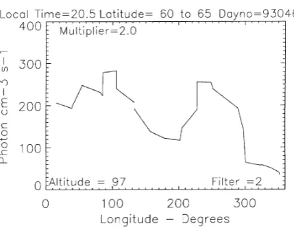
Fig. 7(b). Green line volume emission rate at 95 km versus longitude for February 15, 1993.
Fig. 8(a). Green line emission rate profile for February 15, 1993 at 100◦ longitude and 63◦N.
Fig. 8(b). Green line emission rate profile for February 15, 1993 at 295◦ longitude and 63◦N, a profile that is dominated by aurora.
associated with polar cap ionospheric patches. The volume emission rate errors are much smaller than these F-region features; standard deviations are about 1 photon s−2cm−3. A profile of the volume emission rate standard deviation has been shown by Shepherdet al.(1997), along with another example of F-region green line emission. The profile of Fig. 8(b) is completely different, and is characteristic of au-rora. For a discussion of auroral profiles the reader is referred to the paper by M. Shepherdet al.(1996). The longitude of 250◦corresponds to the longitude of the magnetic pole so is where the aurora has its greatest equatorward extent in ge-ographic coordinates. Airglow emission may be present in this profile; it cannot be distinguished from the dominant au-roral profile, but it is clear that the airglow volume emission rate must be much less than in Fig. 8(a). These two profiles confirm that the wave 1 with its peak near 100◦longitude is an airglow phenomenon, while the second peak near 240◦in the green line data is due to aurora.
On February 16, there were only green line data, which are shown in Fig. 9. The peak emission rate at 100◦
longi-Fig. 9. Green line volume emission rate at 95 km versus longitude for February 16, 1993.
Fig. 10(a). Green line emission rate profile for February 16, 1993 at 99◦ longitude and 62◦N, at the peak of the planetary wave 1 feature.
in phase. The springtime transition is a transition between high winter and low summer values of atomic oxygen that takes place in about one week and is seen most clearly at high latitudes. At mid and low latitudes the dominant effect is the appearance of planetary scale waves which span the equator. Extremely large planetary scale disturbances may be seen at high latitudes during winter. Examination of one event leads to the tentative conclusion that it is the result of a stratospheric warming. The perturbation occurs about two days earlier in the lower thermosphere than in the strato-sphere, and is shifted by about 30◦in longitude between the two levels.
A discussion of the possible connection between the strato-spheric warming and the enhancement of O(1S) emission in the lower thermosphere is beyond the scope of this pa-per. However we note that Dunkerton et al. (1981) pro-vide a model demonstration of the coupling between the stratosphere and mesosphere; the stratospheric warming is accompanied by a mesospheric cooling. It therefore seems reasonable to expect coupling to the lower thermosphere as well, which is strongly implied by the WINDII observations, which indicate thermospheric downwelling in the region of the stratospheric warming, as part of a global-scale wave 1. Dunkertonet al.(1981) point to observations that hint at pre-conditioning of the mean flow by the action of wave 1, as a precursor to the involvement of wave 2 in a major warming. They thus suggest that the essential role of the wave 1 may be to change the mean flow in a way as to focus any upward-propagating wave 2 into the polar cap. Whether the WINDII wave 1 observations are related to this wave 1 precursor is a matter that remains to be explored.
Acknowledgments. The WINDII project is supported by the Canadian Space Agency, and the Centre National d’Etudes Spatiales of France. Scientific analyses of the data are funded by the Natural Sciences and Engineering Research Council of Canada. Nikolas Pertsev first drew our attention to the date of February 15, 1993 as being anomalous in its airglow characteristics.
References
Angelats i Coll, M. and J. M. Forbes, Dynamical influences on atomic oxygen and 5577 ˚A emission rates in the lower thermosphere,Geophys. Res. Lett.,25, 461–464, 1998.
Burrage, M. D., N. Arvin, W. R. Skinner, and P. B. Hays, Observations of the O2atmospheric band nightglow by the High Resolution Doppler
Imager,J. Geophys. Res.,99, 15017–15023, 1994.
Christophe-Glaume, J., ´Etude de la raie 5577 ˚A de l’oxygene dans la lumi-nescence atmosph`eric nocturne,Ann. Geophys.,21, 1, 1965.
Cogger, L. L., R. D. Elphinstone, and J. S. Murphree, Temporal and latitu-dinal 5577 ˚A airglow variations,Can. J. Phys.,59, 1296–1307, 1981. Donahue, T. M., B. Guenther, and R. J. Thomas, Distribution of atomic
oxy-gen in the upper atmosphere deduced from Ogo 6 airglow observations,
J. Geophys. Res.,78, 6662–6689, 1973.
Dunkerton, T., C.-P. F. Hsu, and M. E. McIntyre, Some Eulerian and La-grangian diagnostics for a model stratospheric warming,J. Atmos. Sci.,
38, 819–843, 1981.
McDade, I. C.,et al., ETON 2: Quenching parameters for the proposed precursors of O2(b1!+g) and O(1S) in the terrestrial nightglow,Planet.
Space Sci.,34, 789–800, 1986.
McLandress, C., G. G. Shepherd, and B. H. Solheim, Satellite observations of thermospheric tides: results from the Wind Imaging Interferometer on UARS,J. Geophys. Res.,101, 4093–4114, 1996.
Naujokat, B., K. Petzoldt, K. Labitzke, R. Lenschow, B. Rajewski, M. Wies-ner, and R.-C. Wohlfart, The stratospheric winter 1991/92, Beilage zur Berliner Wetterkarte, Wissenschaftliche Einrichtung 07 im Fachbereich Geowissenschaften der Freien Universitat Berlin, ISSN 0938-5312, 1992. Reed, E. I. and S. Chandra, The global characteristics of atmospheric emis-sions in the lower thermosphere and their aeronomic implications, J. Geophys. Res.,80, 3053–3062, 1975.
Roble, R. G. and G. G. Shepherd, An analysis of Wind Imaging Interfer-ometer observations of O(1S) equatorial emission rates using the
Thermo-sphere-Ionosphere-Mesosphere-Electrodynamics General Circulation Model,J. Geophys. Res.,102, 2467–2474, 1997.
Shepherd, G. G., et al., WINDII: The Wind Imaging Interferometer on the Upper Atmosphere Research satellite,J. Geophys. Res.,98, 10,725– 10,750, 1993.
Shepherd, G. G., C. McLandress, and B. H. Solheim, Tidal influence on O(1S) airglow emission rate distributions at the geographic equator as
observed by WINDII,Geophys. Res. Lett.,22, 275–278, 1995. Shepherd, G. G., R. G. Roble, C. McLandress, and W. E. Ward, WINDII
observations of the 558 nm emission in the lower thermosphere: the influence of dynamics on composition,J. Atmos. Solar-Terr. Phys.,59, 655–667, 1997.
Shepherd, G. G., R. G. Roble, S.-P. Zhang, C. McLandress, and R. H. Wiens, Tidal influence on midlatitude airglow: Comparison of satellite and ground-based observations with TIME-GCM predictions,J. Geo-phys. Res.,103, 14741–14751, 1998.
Shepherd, G. G., J. Stegman, P. Espy, C. McLandress, G. Thuillier, and R. H. Wiens, Springtime transition in lower thermospheric atomic oxygen, J. Geophys. Res.,104, 213–223, 1999.
Shepherd, M. G., R. L. Gattinger, Y. Rochon, G. G. Shepherd, B. H. Solheim, and D. J. W. Kendall, Auroral Observations with the WIND Imaging Interferometer (WINDII) on UARS,Adv. Space Res.,17, (11)5–(11)10, 1996.
Stegman, J., D. Murtagh, and G. Witt, Extremes of oxygen airglow inten-sity, Abstract SA22C-11,AGU Spring Meeting Program, Montreal, May, 1992.
Tohmatsu, T.,Compendium of Aeronomy, translated by T. Ogawa, 509 pp., Terra Scientific Publishing Company, Tokyo, Kluwer Academic Publish-ers, Dordrecht, 1990.
Ward, W. E., A simple model of diurnal variations in the mesospheric oxygen nightglow,Geophys. Res. Lett., 1999 (in press).
Yudin, V. A., M. A. Geller, B. V. Khattatov, D. A. Ortland, M. D. Bur-rage, C. McLandress, and G. G. Shepherd, TMTM simulations of tides: Comparison with UARS observations,Geophys. Res. Lett.,25, 221–224, 1998.
Zhang, S. P. and G. G. Shepherd, The influence of the diurnal tide on the latitudinal distributions of the O(1S) and OH emission rates observed by
WINDII on UARS,Geophys. Res. Lett.,26, 529–532, 1999.