Analysis of hidden terminal’s effect on the performance of vehicular ad hoc networks

R E S E A R C H

Open Access

Analysis of hidden terminal

’

s effect on the

performance of vehicular ad-hoc networks

Saurabh Kumar

, Sunghyun Choi

and HyungWon Kim

Abstract

Vehicular ad-hoc networks (VANETs) based on the IEEE 802.11p standard are receiving increasing attention for road safety provisioning. Hidden terminals, however, demonstrate a serious challenge in the performance of VANETs. In this paper, we investigate the effect of hidden terminals on the performance of one hop broadcast communication. The paper formulates an analytical model to analyze the effect of hidden terminals on the performance metrics such as packet reception probability (PRP), packet reception delay (PRD), and packet reception interval (PRI) for the 2-dimensional (2-D) VANET. To verify the accuracy of the proposed model, the analytical model-based results are compared with NS3 simulation results using 2-D highway scenarios. We also compare the analytical results with those from real vehicular network implemented using the commercial vehicle-to-everything (V2X) devices. The analytical results show high correlation with the results of both simulation and real network.

Keywords:Vehicular ad-hoc networks, Medium access control (MAC), Broadcast communication, Hidden terminal

1 Introduction

Vehicular communication known as vehicle-to-everything (V2X) is an integral part of the intelligent transportation system (ITS) for vehicle safety applications. For wireless communication among the vehicles and vehicle to the roadside unit (RSU), this paper considers communications based on dedicated short-range communication (DSRC) [1]. DSRC uses a band at 5.9 GHz with a bandwidth of 75 MHz. It transmits the basic safety message (BSM) at the center frequency of 5.89 GHz, which is the control chan-nel (CCH) with a bandwidth of 10 MHz. DSRC allows a large number of vehicles and RSUs to communicate among each other, which construct a highly dynamic ve-hicular ad-hoc network (VANET).

DSRC utilizes IEEE 802.11p, which is an amendment of the physical and medium access control (MAC) layers of IEEE 802.11a [2]. The physical layer is based on the or-thogonal frequency division multiplexing (OFDM) modu-lation, while the MAC layer is ameliorated for the low overhead communication. Vehicles in 802.11p communi-cate using the independent basic service set (IBSS) archi-tecture. Thus, it does not require the initial setup phase

for the vehicle’s association [2]. To obtain optimum performance, 802.11p is optimized for the highly mobile environment, fast-changing multi-path reflection, and Doppler shift (due to high relative speed).

The MAC protocol of IEEE 802.11p uses carrier sense multiple access with collision avoidance (CSMA/CA) ran-dom access mechanism as a basic access scheme. To avoid collisions, the CSMA/CA mechanism uses distributed co-ordination function (DCF) to access the channel [2].

In VANETs or V2X based on DSRC, each vehicle transmits BSM packets periodically [1]. BSM is a beacon message that contains the status, position, and move-ment information of the vehicle [1]. Since the transmit-ter broadcasts its BSM to all its neighbor vehicles, the transmitter cannot get the confirmation of the correct reception from the receivers. Because unlike unicast, which can efficiently utilize acknowledgment (ACK) packet, the regular broadcast communication does not support ACK.

The data received in the BSM packets are utilized by the safety applications, thus making the timely packet delivery an utmost performance goal. One of the leading causes of performance degradation in the IEEE 802.11 networks is hidden terminal collisions [3]. Thus, IEEE 802.11 networks use request to send / clear to send (RTS/CTS) mechanism to alleviate the hidden terminal

© The Author(s). 2019Open AccessThis article is distributed under the terms of the Creative Commons Attribution 4.0 International License (http://creativecommons.org/licenses/by/4.0/), which permits unrestricted use, distribution, and reproduction in any medium, provided you give appropriate credit to the original author(s) and the source, provide a link to the Creative Commons license, and indicate if changes were made.

* Correspondence:[email protected]

1_{Department of Electronics Engineering, Chungbuk National University,} Cheongju, Chungcheongbuk-do, South Korea

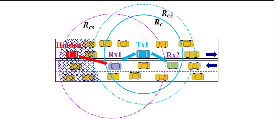
problem [4]. However, the RTS/CTS mechanism is in-applicable in broadcast communication because unlike the unicast, the transmitter of the broadcast communi-cation cannot receive CTS (same as an ACK) from all the receivers, individually. The nodes located within the channel sensing range from a receiver but are out of the channel sensing range from the transmitter, are called hidden terminals for the receiver-transmitter pair. For

example, in Fig. 1, node Tx1 transmits a BSM data

packet. Both the receivers Rx1 and Rx2 in the communi-cation range of the node Tx1 are expected to receive the transmitted packet. However, if the nodes in the shaded area start transmitting their packets at the same time, the receiver Rx1 may not receive the packet correctly. Hence, the nodes in the shaded area are the hidden ter-minals for the node Rx1 (which can be different from the hidden terminals for the node Rx2). Therefore, all the receivers of the broadcast packet independently ex-perience the hidden terminal problem. Therefore, the total region of hidden terminals is sizable. Moreover, in the absence of ACK for the broadcast packet, hidden terminals cannot deduce the transmission1 even from the receiver nodes; hence, the vulnerable period (the time at which the hidden terminals’transmission can re-sult in a collision) can be longer than the unicast com-munication [3].

The packet delivery performance in the case of BSM is determined by the ability of 1-hop receivers to receive the generated packets with high probability within allowed time.

Literature in the hidden terminal analysis can be classified in two types based on the communication category: hidden terminal analysis in unicast communication and hidden terminal analysis in broadcast communication. Many re-searchers have investigated the former. Firstly, Tobagi et al. investigated the effect of hidden terminals on the perform-ance of the network with multiple transmitters and a single receiver in a saturated traffic case [5]. Subsequently, Ray et al. derived the analytical expressions for the packet collision probability, average packet delay, and maximum throughput for the saturated traffic condition [6]. The authors have used the queuing theoretical analysis in a 4-node segment network. Afterward, in [7], Ekici et al. esti-mated the performance under the hidden node problem in the unsaturated traffic conditions for a 3-node symmetric network. Similarly, Tsertou et al. presented the perform-ance modeling of the hidden terminal problem in a 3-node symmetric network using fixed length timeslot [3].

The authors of [8–16] analyzed the performance of hid-den terminals for IEEE 802.11p broadcast communication.

Ma et al. derived the performance metrics for one hop broadcast communication of VANET comprising hidden nodes in [8, 9]. They also analyzed the channel capacity using signal-to-interference ratio (SIR) in VANET under the hidden terminals, access collisions, as well as channel propagation in [10]. However, the authors assumed that the nodes travel in a 1-D highway. Similarly, Fallah et al. analyzed the hidden node interference for the perform-ance of cooperative vehicle safety system in 1-D network [11]. Rathee et al. analyzed the throughput of VANET with hidden terminals in smaller networks of 5 or 10 nodes [12]. Furthermore, Song presented an analytical model for the performance analysis of multichannel MAC in 1-D VANET with hidden terminals [13]. Whereas, au-thors in [14–16] analyzed the hidden terminal problem in 2-D VANET, Ma et al. analyzed the effect of hidden ter-minals for 2-D networks in rural intersections in [14] and for a general 2-D VANET in [15]. In addition, Wang et al. analyzed the performance of enhanced distributed channel access (EDCA) mechanism for 2-D wireless networks [16]. Moreover, the authors in [17–20] presented the effect of hidden terminals via only simulations. Sjoberg et al. [17] and Tomar et al. [18] defined the hidden terminal problem and simulated the effect on both packet recep-tion rate and throughput. The authors in [19, 20] simu-lated the networks for the received interference power from the hidden terminals. They calculated the effect of the interference power on the safety messages’reachable distance and hidden terminals radius. In contrast, the proposed protocol has the following advantages.

Our protocol uses multi-lane 2-D VANET to derive the analytical model, which increases accuracy. Our new Markov chain accurately emulates multiple

backoff counter freezing due to sequential transmission from more than one vehicle in the channel sensing range.

We consider both the communication range and channel sensing range to effectively differentiate the communicating nodes from interfering nodes. Our proposed analytical model uses the fixed length

timeslots; hence, can accurately quantify the collisions from the unsynchronized hidden terminals.

2 Methodology

The analytical model that can evaluate the performance of VANETs under various configurations of network parameters is derived. We then evaluate the accuracy of the proposed model through a comparison with the simulation results based on NS3 using multi-lane high-way scenarios. Additionally, the model’s accuracy is also compared with the results of a real network.

1

The analysis presented in [8–10] assumes the variable size timeslots, which is an extension of the prominent work done by Bianchi [4]. Bianchi assumed that the state transition for all the nodes occurs altogether. This as-sumption is valid for the connected networks since the nodes are synchronized. In the IBSS network with hidden terminals, nodes are unsynchronized; hence, we cannot assume that the nodes start transmission, simul-taneously. In this paper, we consider the fixed-size slots, which are also assumed in [3], where the authors have analyzed the hidden terminals but only in the case of saturated unicast communication with a 3-node net-work. Additionally, in [3], a transmitter node can freeze its counter only once, i.e., there is only one other trans-mitter in the wireless sensing range. In the VANET, however, multiple nodes in the wireless sensing range can transmit the packets one after another. Thus, the counter can freeze multiple times for the same backoff counter value. We design a new Markov chain that can accurately emulate this behavior. We first define the den terminal problem and then model the effect of hid-den terminals on three performance metrics: (1) packet reception probability (PRP), (2) packet reception delay (PRD), and (3) packet reception interval (PRI).

The rest of the paper is organized as follows: Section3 depicts the operation of DSRC MAC for BSM broadcast. Section 4 introduces the system model and outlines the assumptions made in the analytical model. Then, Section

5 defines the hidden terminal problem in 2-D VANET

and derives the model for performance metrics. Section 6evaluates the accuracy of the proposed model in com-parison with the results from NS3 simulator and real network. Section7presents the conclusions.

3 Dedicated short-range communication MAC This section presents the salient facets of the IEEE 802.11p DCF MAC used by the IBSS architecture [2]. Here, only the broadcast communication is considered for simplicity.

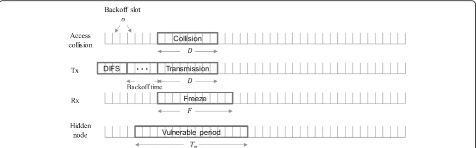
Once the MAC receives a new packet for transmis-sion from BSM application. It starts the transmistransmis-sion process by sensing the channel (using only physical carrier sensing, since virtual carrier sensing is in-applicable in broadcast communication) for the dis-tributed interframe space (DIFS) time. If the channel is idle, the MAC transmits the packet. In contrast, if the sensing result gives channel busy during the DIFS, it continues to wait until the channel becomes idle for the DIFS time. Afterward, the MAC chooses a random backoff counter and delays the transmission for the backoff time as shown in Fig. 2. The backoff time is calculated by the backoff counter multiplied by the timeslot length σ. The counter is drawn from the uniform random distribution between 0 and con-tention window value. Concon-tention window varies from the minimum value to the maximum value, according to the binary exponential backoff (BEB) procedure [2]. In the case of broadcast communication, however, the transmitter is not notified for the unsuccessful trans-missions (no retransmission). Hence, MAC uses the constant contention window (CCW), i.e., the

mini-mum contention window size (W0). The random

backoff time is used to mitigate the access collisions with the nodes in the channel sensing range. Here, an access collision is defined as the collision that occurs when two (or more) nodes in the channel sensing range transmit in the same timeslot.

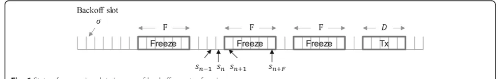
Backoff counter is decremented at the start of each timeslot (also called backoff slot) of lengthσ, only if the channel is sensed idle. If the channel is busy, on the other hand, the backoff counter freezes for the sensed packet transmission plus DIFS time. Afterward, the MAC resumes decrementing the counter. Once the counter reaches zero, the node transmits the packet at the start of the next timeslot. The timeslot length σ is the sum of the time needed for the channel assessment, MAC processing delay, time to switch the transceiver from receiving to transmitting mode, and propagation delay [2]. After finishing the transmission, the node de-lays the next packet transmission for the random backoff time. This strategy allows a fair use of channel among all the neighbor nodes.

4 System model and modeling assumptions To derive the system model, we assume that the vehicu-lar nodes are randomly distributed in a multi-lane high-way having a total ofξlanes (including both directions). The width of each lane isω. Vehicle’s initial placement in the highway follows the poison point process (see Fig. 1) and its density is α vehicles/lane/km. However, their movement (vehicle speed with respect to time) ex-hibits exponential distribution [21] and constructs a highly dynamic 2-D VANET. The notation of node, ter-minal, or vehicle is used interchangeably. Additionally, the slot and timeslot both mean one timeslot of length σ. Frequently used notations in the model are specified in Table 1, and the descriptions of important notations are given as follows.

BSM application in each node generates safety data packet periodically atλHz rate. The packet is generated at the start of the new period and stored in the MAC queue. Subsequently, DCF MAC starts the transmission process. Thus, the packet arrival to the MAC queue follows the deterministic

Fig. 2Operation of 802.11p MAC as well as access collision and hidden terminal collision along with their operation time

Table 1Most frequently used modeling notations

Notation Description

ξ Total number of lanes

ω Width of the lane (m)

α Vehicle density (vehicles/lane/km) D BSM application data packet size (bytes)

⌈x⌉ Ceil(x): smallest integer greater than or equals tox SD Symbol duration (μs)

R Data rate (bits/s)

TDATA Time required to transmit a data packet

SDATA Number of timeslots needed to transmit the data packet

σ Size of the timeslot (μs)

Rc Communication range (m)

Rcs Channel (carrier) sensing range (m) (1.5 ×Rc) Nc Number of nodes in the communication range Ncs Number of nodes in the channel sensing range λ Packet generation rate in each node (Hz)

V Set of vehicular nodes

C Set of communication sets of the nodes

H(vi,vj) Set of hidden terminals for the transmitterviand receivervj pair

Ph Probability of collision due to hidden terminals PTx Probability of transmission in a slot

Nh Average number of hidden terminal nodes for 2-D VANET

Tvul Vulnerable time

Svul Number of slots in the vulnerable time Pd Probability of data availability in the MAC queue b(s) Value of backoff counter at statesin the Markov Chain f(s) Value of freezing slot at statesin the Markov Chain τ Stationary probability of data transmission in a slot

MD Average (mean) MAC delay

W0 Constant contention window size

distribution. For modeling simplicity, this paper assumes an infinite size MAC queue because none of the packets are dropped due to queue full condition. Each packet is transmitted after the backoff time, which follows semi-Markov service time. Therefore, the MAC queue follows (D/M/1) queuing model ([22], p377), where 1 indicates the number of channels used (only CCH).

Figure3shows the details of the transmitted BSM packet. Let the size of BSM packet generated by the safety application isDbytes. The network and the MAC layers addHNetandHMACbytes, respectively, for the network header and MAC header. On top of that, the MAC layer also addsH_Trailbyte frame check sequence (FCS) trailer information. Finally, the physical layer adds physical layer convergence procedure (PLCP) preamble (4 symbols), PLCP header (1 symbol), 16 bits service detail and 6 tail bits [2].

The PLCP preamble and PLCP header are transmitted using the binary phase shift keying (BPSK) with 1

.

2 code rate. It requires constant duration irrespective of the employed data rate. However, the rest of the packet is transmitted using physical layer data rate, which isR(bits/s).

If one symbol duration isSD. The number of data bits transmitted per symbol areR×SD. Therefore, the number of symbols (NS) in a packet are,

Hence, the total time needed to transmit the data is,

TDATA¼ 5þ

The number of timeslots needed to transmit the data packet can be calculated from Eq. (3).

SDATA¼ TDATA_σ

ð3Þ

If nodev_isenses transmission from the nodes within vi’s channel sensing range,vifreezes its backoff counter for the packet transmission plus DIFS time. Hence, the freezing time isTDATA+ DIFS. Thus, the number of freezing slots is given as follows.

F¼SDATAþ

DIFS σ

ð4Þ

For tractability and simplicity of the model, the follow-ing assumptions are made:

All the nodes are identical and have a uniform circular communication rangeR_cand channel (carrier) sensing rangeRcs(Rc<Rcs< 2 ×Rc). All the nodes in the communication range of the

transmitter can receive the packet correctly. However, the nodes in the channel sensing range can detect the transmission but might not be able to decode the packet contents correctly. The number of nodes in the communication range (Nc) and the channel sensing range (Ncs) are derived in the

Appendix.

We consider only BSM safety data transmission over continuous mode 802.11p MAC. In the continuous mode, the radio transceiver of the vehicle is always in operation at CCH for whole 100 ms [2].

We do not consider shadowing, fading, and channel capturing in the modeling for simplicity. The focus of the paper is on the effect of hidden terminals in the 1-hop broadcast communication.

5 Modeling of hidden terminal problem

Unlike unicast, the safety data in the DSRC is broad-casted so that each node in the communication range of the transmitter is a prospective receiver. The hidden ter-minal problem in broadcast communication is different from that in unicast communication. For the broadcast of a transmitter, a set of nodes can be hidden terminals

for a receiver and might not be for others. For example, in Fig. 1, for the transmission of Tx1, the nodes in the shaded area are the hidden terminals for the receiver Rx1, whereas they are not the hidden terminals for the receiver Rx2. Although the authors in [17, 18] defined the hidden terminal problem, they had not considered channel sensing range, which in general, is larger than the communication range.

We represent a 2-D VANET by an undirected graph G= (V,C), where V is the set of all vehicular nodes in the network. We can ignore the effect of mobility during the packet transmission since it takes a very short time (< 1 ms) for the vehicle to transmit a short packet like BSM [9]. Therefore, a vehicular nodevi∈Vis positioned

at ðxvi;yviÞ, and assumed to be stationary for the trans-mission time.

We define C as a set of communication set nodes,

expressed by Eq. (5).

C¼fcvijvi∈Vg ð5Þ

Here, communication set cvi for the nodeviis the set of all the nodes in the communication range of the node vi for a transmission instant. In other words, cvi is the set of prospective receivers for the current transmission from the nodevi, which is denoted by Eq. (6).

whered(vi,vj) denotes the Euclidean distance between

the nodesviandvj.

If node vi is transmitting a packet and node vj is one

of the intended receivers among cvi. The set of hidden terminals for the transmitter-receiver pair is expressed by Eq. (8). range and other notations are described in Table1.

During the transmission from the node vi, if any node

in the set H(vi,vj) transmit at the vulnerable period, vj

experiences collision thus, cannot receive the packet, correctly. This is called the hidden terminal problem in the broadcast communication for the vehicular ad-hoc networks and such collisions are called hidden terminal collisions. The probability of hidden terminal collision Ph is the probability of at least one of the hidden

terminal nodes transmitting at the vulnerable period. Ph

can also be derived from the probability of none of the hidden terminal nodes transmit in the vulnerable timeslots.

Ph ¼1− ð1−PTxÞNh

Svul

ð9Þ

Here, PTx is the probability of transmission in a

time-slot, Nhrepresent the average number of hidden

termi-nals for the transmitter-receiver pair, and Svul is the

number of timeslots in the vulnerable period. To analyze the effect of hidden terminals using Eq. (9), we derive PTx,Nh(in theAppendix) andSvul.

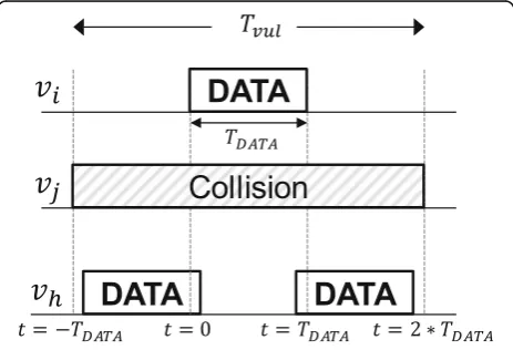
5.1 Vulnerable time period (Tvul)

Unlike [4], the vehicular nodes in VANET are not con-nected with the common base station, and thus they are unsynchronized. Therefore, the start of transmission in the nodes is also unsynchronized. The time period when the hidden terminals’ transmission can collide with the

ongoing transmission is called vulnerable period

Tvul [13]. Unicast communications exert ACK, which is

received by the hidden terminals, and thus, they can suppress transmission. Hence, the vulnerable period in unicast communication is smaller [3]. For broadcast communications,Tvulcan be expressed by Eq. (10).

Tvul¼3TDATA ð10Þ

Here,TDATAis the data packet transmission time.

As shown in Fig.4, we assume the nodevistarts

trans-mission att= 0. Since nodes are not synchronized in the VANET, we can infer from Fig. 4 that any transmission from the hidden terminals (vh) in the interval (-TDATA,

2 ×TDATA) results in a collision at the receiver vj.

How-ever, if the hidden terminal node vh transmits before

(-TDATA) or after (2 ×TDATA), the receiver vj receives

the transmitted packet from the transmitter vi without

hidden terminal collisions.

The number of timeslots in a vulnerable period can be calculated by Eq. (11) using the vulnerable time period from Eq. (10).

Svul¼ T_σvul

ð11Þ

5.2 Probability of transmission in a slot (PTx)

The hidden terminals for the pair of transmitter and receiver lie within the channel sensing range of the receiver. Therefore, while calculating the probability of transmission, the cascading effect of the hidden termi-nals is not envisaged.

The probability of transmission in a timeslot for the unsaturated traffic in a node depends on the following two independent probabilities: (1) data arrival probability or data availability in the MAC queue (Pd), (2) the

sta-tionary transmission probability in a timeslot (τ). Hence, the probability of transmission in a slot can be written as Eq. (12).

PTx ¼Pdτ ð12Þ

However, two or more hidden terminals transmitting in the same slot can result in access collision among hid-den terminals. Thus, the probability of successful packet transmission in a slot is expressed by Eq. (13).

PS¼Pdτð1−pÞ ð13Þ

Here, p is the conditional collision probability (access collisions) given the node transmits in a timeslot.

5.3 Probability of data availability (Pd)

Data packet arrival at the MAC queue is deterministic with the rateλHz and service time is exponential (semi-Markov) with the mean MAC delayMD. Hence, the data

availability in the MAC is a stochastic process with the Poisson distribution. As a result, the probability mass function (PMF) of the number of packets in time tcan be written by Eq. (14) ([22], p 307).

pnð Þ ¼t e−λt λt

ð Þn

n! ; wheren>0 ð14Þ If the application generates a new packet before the current packet is transmitted, the current one becomes obsolete. Hence, after the generation of the next packet existing packet is preempted from the queue. Thus, the MAC queue always contains either one packet or zero packets. Hence, the probability of data availability is the

PMF of one packet in the queue in the mean MAC delay MD, which is calculated using Eq. (15).

Pd¼e−λMDλMD ð15Þ

Section 5.6derives the mean MAC delay MD; for the

BSM packet. The network is unsaturated if the traffic follows λ_MD <1 condition. However, it becomes satu-rated if λMD≥1 , and the MAC queue start preempting

non-transmitted packets.

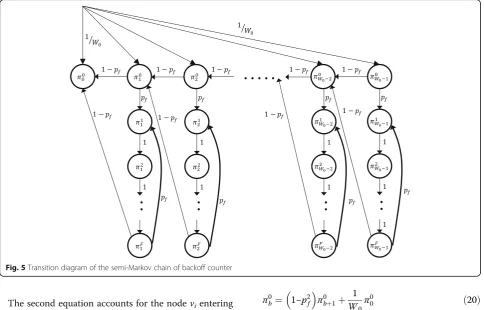
5.4 Stationary transmission probability in a slot (τ) We derive the stationary probability of transmission in a given slot (τ) for a node by using the Markov chain model of backoff counter transition. The timeframe is divided into discrete timeslots of a fixed length σ. Lets, and s+ 1 are two consecutive timeslots. Initially, a ve-hicle vi chooses its backoff counter from the uniform

random distribution of [0,W0). The backoff counter ofvi

is decremented at the start of the next timeslot s+ 1 if the channel is sensed idle in the timeslot s. However, if any other node in the carrier sensing range starts trans-mitting with probability pf, the channel becomes busy,

and hence, the backoff counter of vi freezes with the

current value. The counter continues to freeze for the nextFtimeslots. Afterward, the counter starts to decre-ment, if the channel becomes idle, which occurs with probability (1−pf). However, if any other node starts

transmitting after F slots, the backoff counter of vi

re-mains the same and continues to freeze for the next F slots. The transition process of the Markov chain is de-scribed in Fig.5. The non-null transition probabilities of individual steps in the Markov chain are given by Eq. (16)2.

The first three equations in Eq. (16) account for transi-tion related to freezing slots. The first equatransi-tion repre-sents the transition from the first freezing slot until the last (Fthslot). Once the node vi starts sensing the

The second equation accounts for the nodevientering

the freezing process. Oncevisenses channel as busy with

probability pf, which occurs when other nodes in the

carrier sensing range of vi start the transmission, the

counter ofvifreezes for the nextFslots.

Equation three accounts for the continuation of the freezing process of the backoff counter for the next F timeslots, if any other nodes start transmitting after the current node finishes. The 4th and 5th equation account for decrementing the backoff counter; the former without going to freezing states and the latter after completing the freezing states, respectively. The last equation accounts for the initial backoff counter selection, once a new packet arrives in the MAC queue for the transmission.

Letπ_bf ¼ lim

t→∞PfkðsÞ ¼b;lðsÞ ¼fg;b∈ð0;W0−1Þ;f∈ð0

;FÞ be the stationary probability of the states in the semi-Markov chain. From the closed form solution, we can derive Eqs. (17) and (18).

π1

Solving Eqs. (17) and (18) gives Eq. (19).

πf

Another closed form solution from the backoff coun-ter decrement states can be expressed by Eq. (20).

π0

Eq. (20) can be simplified to Eq. (21).

π0

Eqs. (19) and (21) illustrate the values of the stationary probabilities π_bf of Markov states in terms ofπ0

0 and the freezing probability pf. By using the Markov chain

normalization condition, we determineπ0

0as follows.

The vehicular node transmits in the next slot after the backoff counter becomes zero. Hence, the stationary transmission probability in a slot can be calculated by Eq. (24).

τ¼π0

If we consider backoff counter transition without freezing (_pf= 0), a solution can be obtained by using a

Markov chain based on classical constant contention window [4]. The stationary probability of transmission in a slot with_pf= 0 can be expressed by Eq. (25).

τ¼ 2

W0þ1

ð25Þ

5.5 Freezing probability (pf)

xTo derive τfrom Eq. (24), we require pf, freezing

prob-ability of the backoff counter for the nodeviin a slot. The

counter freezes, when at least one of the nodes (Ncs−1)

within the channel sensing range from vi transmit in a

backoff slot. The backoff counter is chosen from [0,W0−

1] based on the uniform random distribution. Hence, the

probability of a backoff slot selection is 1 .

W0

. As a

re-sult, the probability that at least one of the nodes choose

the given backoff slot isð1−ð1−1

then the backoff counter continuously freezes for the next Fslots, till slotSn+F. As a result, the nodes in the sensing

range do not transmit in the next F slots, which means that only one out of F slots has a freezing likelihood. Hence, the freezing probability is calculated as Eq. (26).

pf ¼

Once the MAC queue receives a new packet (the previ-ous packet is flushed if not transmitted), it starts the transmission process by choosing a backoff counter. Based on the channel state (idle or busy), the MAC dec-rements the backoff counter from the chosen value until zero. As soon as the counter becomes zero, the MAC

transmits the packet in the next slot. Henceforth, the mean MAC delay for the packet is the average time spent in the Markov chain of the backoff counter transi-tion. Markov chain consumes time in two states: (1) time in the freezing states in case of transmissions from the other nodes and (2) time consumed in decrementing the backoff counter until zero in the idle channel state. LetBbe the random variable for the backoff counter se-lection, then the MAC delay for a packet is written by Eq. (27).

MD ¼pf FσBþσB ð27Þ

To obtain the mean MAC delay, we take the expect-ation on both sides of Eq. (27), which leads to Eq. (28).

E M½ D ¼ pf Fþ1

σE B½ ð28Þ

The expected value of the MAC delay is MD and the

expected value of the random variable of CCW backoff counter with range [0,W0−1] isW0

.

2. After substitut-ing values in Eq. (28), we can obtain MD expressed by

Eq. (29).

MD ¼ pf Fþ1

σW0

2 ð29Þ

The effect of hidden terminal collisions on the per-formance metrics PRP, PRD, and PRI are expressed in the following subsections using the probability of hidden terminal collision (Ph) obtained by Eq. (9).

5.7 Packet reception probability (PRP)

Packet reception probability is the ability of 1-hop re-ceiver nodes to receive the BSM packet generated at the transmitter vehiclevisuccessfully. Hence, it is measured

as the probability of packets received with respect to the packets generated by the vehicles in the communication range. The receiver does not receive the transmitted packets if lost due to collision. Hence, the hidden ter-minal collisions directly affect the PRP. The loss in the PRP due to hidden terminals is the same as the probabil-ity Phof hidden terminal collision at the receiver. As a

result, the effect of hidden terminals on PRP can be cal-culated using Eq. (30).

PRP¼1−Ph ð30Þ

5.8 Packet reception delay (PRD)

Packet reception delay is defined as the time lapse be-tween the packet arrival at the MAC queue of the trans-mitter and the packet reception in the MAC queue of the receiver. PRD can also be represented as MAC-to-MAC delay. For the sake of simplicity, in this paper, we ignore the time delay between the packet generation in the application and the start of the transmission process in the MAC. Thus, the MAC-to-MAC delay can be sim-plified as the sum of DIFS, mean MAC delay (MD), data

packet transmission time (TDATA), packet propagation,

and physical layer processing time (σ). Hence, the aver-age packet delay can be calculated by Eq. (31).

PRD¼DIFSþMDþTDATAþσ ð31Þ

5.9 Packet reception interval (PRI)

The efficiency of the safety applications depends on the freshness of the BSM data received from the neighbor nodes. The freshness of the BSM data depends on the rate of packet reception at the receiver, which in turn is affected by the probability of the transmission in a slot, access collision, and hidden terminal collision. We de-fine the packet reception interval at the receiver as the average time between the reception of two consecutive packets from the same transmitter. The value of the packet reception interval should be 1.

λ for the up-to-date data. Let a vehicle vi receive λ′ packets/s from a

transmitter, which is calculated using Eq. (32).

λ0¼λð1−PhÞ ð32Þ

Eq. (32) signifies that the packets lost due to hidden terminal collisions decrease the rate of packet reception.

PRI is, therefore, calculated as 1 .

λ0 by Eq. (32).

6 Model verification

This section analyzes the accuracy of the analytical model and evaluates the effect of hidden terminals in 2-D VANET. Extensive simulation results are exhibited for the performance metrics PRP, PRD, and PRI and compared with the results of the analytical model de-rived in Eqs. (30), (31), and (32), respectively. Further-more, the accuracy of the analytical model is compared with the measured result of a real network of V2X hardware devices.

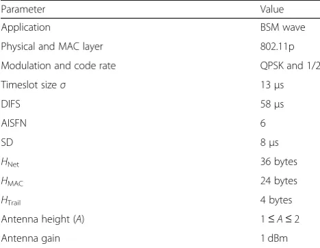
6.1 Simulation setup

The simulations are conducted using the network simu-lator 3 (NS3) [23]. As shown in Fig. 7, the simulator is implemented using a realistic multi-lane highway mobil-ity model. Simulations have been conducted in a 10 km highway segment. The highway model has a total of 10 lanes (5 in each direction) with a lane width of 4 m [24]. Each vehicle is randomly assigned to one of the lanes and kept in that lane throughout the simulation. The speed of the vehicle is assigned based on the lane number: 40 km/h for lane 1, 70 km/h for lane 2, 100 km/ h for lane 3, 120 km/h for lane 4, and 140 km/h for lane 5. As a result, vehicles maintain the same speed during the simulation and do not collide or cross each other. Unless specified, the default data rate for BSM safety data is 6 Mbps and uses quadrature phase shift keying (QPSK) modulation and code rate 1

.

2 for the robust performance.

Other simulation parameters are summarized in Table 2. The channel is simulated using the Nakagami-m propagation Nakagami-model, which is best suited for vehicular communication in highway scenarios [25]. Nakagami-m computes two distance dependent parameters: fading

factor (m) and average power (Ω). Torrent-Moreno

et al. computed the values of m and Ωfor the highway scenario using maximum likelihood estimation [25]. The authors have shown that the average received power (Ω) is inversely proportional to the square of the distance

between the transmitter and receiver (∝1

.

d2 ). In addition, fading parameter mvaries on the basis of dis-tance range. For example, (1)m= 3 for a short distance between the transmitter and receiver (d≤100), (2)m= 1.5 for an intermediate inter-distance (100 <d≤250), and (3)m= 1 for the long distance (d> 250). Up to a tance of 250 m, the propagation follows the Racian dis-tribution (incorporates the line of sight). Beyond that distance, the Rayleigh distribution is employed to calcu-late the average received power. We have chosen the threshold for communication range, and the threshold for channel sensing range as−96 dBm and−99 dBm, re-spectively. The simulations are conducted using BSM packets, which are transmitted in the CCH (Channel number 178) using continuous mode [1]. Each simula-tion result is computed by taking the average of 5 simu-lation readings by using different random seeds and the simulation time for each run is 50 s.

6.2 Real network with commercial V2X devices

for controlling the detailed operations of the packet flow and avoid indeterministic delays. Hence, the network layer headerHnetis zero, while the other parameters are

configured the same as Table 2. Due to a limited num-ber of commercial V2X devices, the results are exhibited for a network of four devices as shown in Fig. 8. The DSRC standard requires that each vehicle generates BSM packet every 100 ms (10 Hz). Thus, we have config-ured both the transmitter Tx1 and Tx2 to generate BSM packets every 1 ms to emulate 100 vehicles in each transmitter. Similar changes are made for other packet generation rates to emulate 100 vehicles per transmitter. Therefore, our network emulation technique can effect-ively measure the performance in a larger network using limited resources. Transmitters Tx1 and Tx2 are acting as hidden terminals for the receiver Rx1 since both transmitters are within the communication range of Rx1. In contrast, Rx2 can receive from Tx1 without col-lision, since the only transmitter, Tx1 is in the commu-nication range of Rx2. The nodes are stationary during the experiment.

There are no access collisions because the two trans-mitters are hidden terminals to each other. The number of hidden terminals Nh for any transmission is always

one (Tx1 when Tx2 is transmitting or Tx2 when Tx1 is transmitting). Additionally, for both transmitters, the number of nodes in the channel sensing rangeNcsis also

one. By using this condition, the probability of freezing (pf) is calculated from Eq. (26) as zero.

6.3 Effect on packet reception probability (PRP)

The collisions due to hidden terminals reduce the

packet reception probability of the transmitted

packets. In the case of the analytical model, the loss in the PRP due to hidden terminals (Ph) is calculated

by Eq. (9). In case of simulation, on the other hand, the loss in the PRP due to hidden terminals (Phs) is calculated using Eq. (33).

Phs¼

Hidden terminal collisions

Expected receive packets ð33Þ

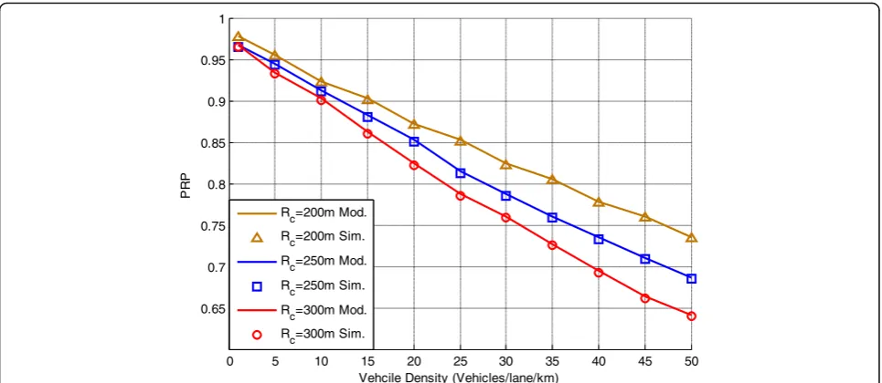
Figure 9 shows the loss of PRP due to hidden

ter-minal collisions for both analytical model and simu-lation, and compares with all types of collisions for the simulation (note that analytical model derives the effect of only hidden terminal collisions). All types of collisions are comprised of both access col-lisions and hidden terminal colcol-lisions. The loss due to all types of collisions (PALL) is calculated by

Eq. (34).

PALL¼

Expected receive packets−actual received packets Expected receive packets

ð34Þ

The comparison results from Fig. 9 manifest that the result of the analytical model closely matches the simu-lation result because we have considered only hidden terminal collisions. The results in Fig. 9 also show that the PRP loss due to hidden terminals increases more rapidly than the access collisions as the vehicle density increases. This result is also evident from Fig.10, which shows that the PRP (only considering the hidden ter-minal collisions) decreases as vehicle density increases.

Figure 10also shows that the reason for the decrease in PRP is due to an increase in the average number of

hidden terminals per receiver as density increases. Fur-thermore, Figs. 11, 12, 13, 14, and 15 demonstrate the similarity in the PRP of the simulations and analytical model (only hidden terminal collisions are considered).

The results in Fig. 11 exhibit that the increase in the minimum contention window size (W0) increases the

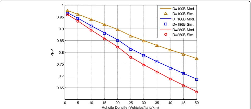
PRP, although the increase is minuscule. The increase is due to an increased number of backoff slots. The results in Fig. 12 show that the PRP can be increased by de-creasing the communication range (transmission power) of the transmitter. The reduction in the transmit power decreases the number of hidden terminal nodes, which leads to increased PRP. The results in Fig. 13 manifest that reducing the BSM data packet size increases the PRP in case of hidden terminals. This is attributed to the reduction in the vulnerable period because of the short packet transmission time.

Figure14presents the PRP measured by changing the packet generation rate of BSM application. The results show that reducing the packet generation rate reduces the contention (packet flow in the wireless channel), which in turn increases PRP. This increase can be ex-plained as, even if the density increases, the total num-ber of packets requested to be transmitted in the channel are not increasing as fast. Hence, the probability that hidden terminals transmit during the vulnerable period decreases.

The results in Fig.15show that by increasing the data rate of the transmitted packet, the effect of hidden ter-minals on PRP can be reduced. Higher data rate reduces the packet transmission time. Due to the reduction in the BSM packet transmission time, the vulnerable period decreases, which has a similar effect as reducing the BSM data size.

Table 2The parameters used in NS3 simulation and devices

Parameter Value

Application BSM wave

Physical and MAC layer 802.11p

Modulation and code rate QPSK and 1/2

Timeslot sizeσ 13μs

DIFS 58μs

AISFN 6

SD 8μs

HNet 36 bytes

HMAC 24 bytes

HTrail 4 bytes

Antenna height (A) 1≤A≤2

Antenna gain 1 dBm

For the experiments with the real network, we calcu-late the loss in PRP (PhN) by Eq. (35).

PhN ¼

packets received at Rx2−packets received at Rx1 packets received at Rx2

ð35Þ

The result of the analytical model for the loss in PRP is calculated using Eq. (9). Figure 16 compares the re-sults measured from the real network with the rere-sults of the analytical model. The results from the real network show the small difference due to non-uniform (circular)

communication range of the transmitter as well as multi-path fading and shadowing. However, the differ-ence is less than 1% compared with the analytical values. The results also exhibit that the density is fixed in the real network. Hence, Fig.16has been plotted for various values of minimum contention window sizes.

Since the MAC layer of the V2X device uses 8-bit un-signed integer for the minimum contention window size; hence, the results can be obtained only up to W0= 128.

The results for the data rate, BSM data size, and packet generation rate also show similarity with the analytical results.

Fig. 9Loss in the PRP due to hidden terminal collisions for the analytical model (Mod.) and simulations (Sim.) and all type of collisions for simulation. The network parameters areW0= 16, R= 6 Mbps,Rc= 250 m,λ= 10 Hz,D= 186 B

6.4 Effect on packet reception delay (PRD)

As described in Section5. H, the packet reception delay for the broadcast packet is defined as MAC-to-MAC delay for the packet. The analytical model calculates the delay by using Eq. (31), whereas the simulation obtains the delay by measuring the average delay between the packet reception time at the receiver and the packet gen-eration time at the transmitter. The time difference is measured using the timestamp added by the transmitter

in the BSM packet. Figure 17 shows the PRD with and

without considering hidden terminal collisions. It shows that the results from the simulation and analytical model closely match, which confirms the high accuracy of the proposed analytical model. Additionally, results also ex-hibit that the hidden terminals have a negligible effect on PRD. This small change is attributed to the fact that the PRD also depends on the time consumed by the MAC queue before transmission. Hence, PRD remains nearly constant irrespective of the hidden collisions. When there is no hidden terminal collision, on the

Fig. 11Comparison of the analytic model and simulation results of PRP with hidden terminal collisions for various minimum contention window sizes with respect to vehicle density,Rc= 250 m, R= 6 Mbps,λ= 10 Hz,D= 186 B

other hand, more packets are received correctly, which smooths out the average PRD value (negligible difference).

Figure 18 compares the PRD results of the real net-work experiment (Fig. 8) and the analytical model. The PRD results are measured at Rx1 and Rx2 for the effect of hidden terminal collisions and without collisions, re-spectively. The results show that the hidden terminals have no noticeable effect on PRD.

6.5 Effect on packet reception interval (PRI)

The packet reception interval is defined as the average time between the reception of two packets at a receiver from the same transmitter. In the analytical model, the PRI is calculated by Eq. (32). In the simulation, the re-ceiver measures the average arrival time difference be-tween two successive packets from the same transmitter. Figure19 compares the PRI calculated by the analytical model and measured by the simulation. The results

Fig. 13Comparison of analytic model and simulation results of PRP with hidden terminal collisions for various BSM data sizes with respect to vehicle density,W0= 16, R= 6 Mbps,Rc= 250 m,λ= 10 Hz

show that the PRI from the analytical model match with the simulation results. It also exhibits that the PRI in-creases with the increase in the density, which incurs due to increased number of hidden terminal collisions. However, increasing the packet generation rate reduces the PRI.

For the real network of Fig.8, the PRI is calculated as the average inter-packet interval for the packets received from the device Tx1 at Rx1 for the hidden terminal case and Rx2 for no collisions case. Figure 20 compares the analytical results with the results measured from the real

network. Figure 20 exhibits that the results from the analytical model closely match the results from the real network. It also shows that the PRI is higher in case of hidden terminals. Additionally, it deduces that the value of the minimum contention window size does not affect the PRI, although increasing the packet generation rate decreases the PRI.

7 Conclusion and future work

In this paper, we proposed an analytical model to evalu-ate the effect of the hidden terminals in 2-D VANET.

Fig. 15Comparison of analytic model and simulation results of PRP with the hidden terminal collisions for data rates with respect to vehicle density,W0= 16, Rc= 250 m,D= 186 B,λ= 10 Hz

The proposed model accurately estimates the perform-ance metrics; packet reception probability (PRP), packet reception delay (PRD), and packet reception interval (PRI) for BSM safety data broadcast for a wide range of realistic vehicular networks. In order to verify the accur-acy of the proposed analytical model, we have used NS-3 simulator with realistic vehicle mobility in various high-way scenarios. Furthermore, we implemented a real ve-hicular network using commercial V2X devices. Our extensive simulations and experiments demonstrated that the performance estimated by the analytical model

accurately matches the performance measured from the NS3 simulator and real hardware network. The analyt-ical model shows only minuscule discrepancy due to variance in the vehicle movement, channel fading and shadowing in the model. The results exhibit a decline in the PRP and PRI metrics’performance, while the PRD is not affected by the hidden terminals.

The metrics PRP and PRI depend on the network pa-rameters; hence, the model can be used in adaptive con-gestion control to reduce the effect of hidden terminal problem. In future work, we plan to use this model as a

Fig. 17Comparison of analytical model and simulation results of PRD with the hidden terminal collisions and without collisions with respect to vehicle density,W0= 16, R= 6 Mbps,Rc= 250 m,λ= 10 Hz,D= 186 B

cost metric to optimize the performance of 2-D VANET under hidden terminals.

8 Appendix

In the Appendix, we first derive the average number of nodes in the communication range (Nc) and channel

sensing range (Ncs). We then calculate the average

num-ber of hidden terminal nodes (Nh) experienced by a

re-ceiver for a 2-D multi-lane highway.

8.1 Number of nodes in the communication range LetXbe a random variable representing the current lane of the vehicle. As shown in Fig. 21, for a vehicle in the xth lane, the number of vehicles in the communication range for each lane varies. Suppose, the vehicle in thexth lane is placed at the origin of 2-D coordinates, and each lane is spaced by one step of lane widthω in the coord-inate system. Let mbe the y-axis value for the distance vector for each lane from the origin. The distance to each lane from the origin can be expressed as |m×ω|.

Fig. 19Comparison of PRI from analytical model and simulation for hidden terminal collisions and without collisions with respect to vehicle density for different packet generation frequencies,W0= 16,R= 6 Mbps,Rc= 250 m,D= 186 B

As a result, the average number of neighbor nodes for a vehicle in thexthlane can be expressed by Eq. (36).

Nc

ð Þ_x¼2α X

ξ−x

m¼1−x

ffiffiffiffiffiffiffiffiffiffiffiffiffiffiffiffiffiffiffiffiffiffiffiffiffiffiffi R2c−ðmωÞ

2 q

ð36Þ

The average number of nodes in the communication range for whole network can be calculated by taking the average of the nodes in the communication range for the transmitters in each lane. Thus, the average number of nodes in the com-munication range can be calculated by Eq. (37).

Nc¼

2αPξ_x¼1Pξ−_m¼x_1−x

ffiffiffiffiffiffiffiffiffiffiffiffiffiffiffiffiffiffiffiffiffiffiffiffiffiffiffi R2

c−ðmωÞ

2 q

ξ ð37Þ

The average number of nodes in the channel sensing range can also be calculated using Eq. (37) by replacing RcwithRcs.

8.2 Number of hidden terminals

Suppose X is the random variable representing the lane of the transmitter node, and Y is the random variable representing the lane of the receiver with respect to the transmitter. In Fig.22, a transmitter inxthlane broadcasts a packet, while a node inythlane is a prospective receiver. Assume that the transmitter node is placed at the origin of 2-D coordinates and that the receiver is positioned at (b,y×ω). Whereωis the lane width. The number of hid-den terminal nodes in the mth lane from the receiver is calculated using Eq. (38) for the transmitter-receiver pair.

hm ¼α bþ

ffiffiffiffiffiffiffiffiffiffiffiffiffiffiffiffiffiffiffiffiffiffiffiffiffiffiffiffi R2

cs−ðmωÞ 2 q

− ffiffiffiffiffiffiffiffiffiffiffiffiffiffiffiffiffiffiffiffiffiffiffiffiffiffiffiffiffiffiffiffiffiffiffiffiffiffiffiR2

cs−ððyþmÞ ωÞ

2 q

ð38Þ The total number of hidden terminal nodes for the transmitter-receiver pair can be calculated by summing the hidden nodes in all the lanes (see Eq. (39)).

Fig. 21Number of vehicles in the communication range calculation for a vehicle inxth_lane

H¼ X

To calculate the average number of hidden terminals in the network, we first calculate the average number of hidden terminalsHyfor the receivers inyth lane. Hycan

be calculated by taking the average of the hidden nodes for all receivers inythlane. The positions of receivers in yth lane can be obtained by changing the coordinate b for all the receivers in the communication range of the transmitter. As a result, Eq. (40) expresses the average number of hidden nodes for the receivers in theythlane.

Hy¼

Eq. (40) can be simplified to Eq. (41).

Hy¼

From Eq. (41), We can derive Eq. (42), which calcu-lates the average number of hidden terminal nodes for all the receivers of the transmitter inxthlane.

Hx¼

Pξ−x y¼1−xHy

ξ ð42Þ

By extending Eq. (42), we can derive Eq. (43), which gives the average number of hidden terminals in the net-work. Here, Nh is obtained by taking the average of the

number of hidden terminals for the transmitters in all the lanes.

ACK:Acknowledgment; BSM: Basic safety message; CCH: Control channel; DSRC: Dedicated short-range communication; MAC: Medium access control; PRD: Packet reception delay; PRI: Packet reception interval; PRP: Packet reception probability; RSU: Roadside unit; RTS/CTS: Request to send/clear to send; V2X: Vehicle to everything; VANET: Vehicular ad-hoc network

Authors’contributions

All three authors contributed equally. SK formulated the analytical model and implemented the simulation and real network. Afterward, together SK, HK, and SC verified the model, generated results, and wrote the manuscript. All authors read and approved the final manuscript.

Funding

This work was supported in part by IITP Grant through the Korean Government, under the development of wide area driving environment awareness and cooperative driving technology which are based on V2X wireless communication under grant R7117-19- 0164 and in part by the Cen-ter for Integrated Smart Sensors funded by the Ministry of Science, ICT & Fu-ture Planning as Global Frontier Project, South Korea (CISS-2019).

Availability of data and materials

Most of the material is taken from the published journals and books, which are referenced. We have also referenced the websites for simulation details and Cohda wireless device specifications.

Competing interests

The authors declare that they have no competing interests.

Author details 1

Department of Electronics Engineering, Chungbuk National University, Cheongju, Chungcheongbuk-do, South Korea.2_{Department of Electrical and} Computer Engineering, Seoul National University, Seoul, South Korea.

Received: 14 March 2019 Accepted: 9 September 2019

References

1. US Federal Communications Commission.Standard specification for telecommunications and information exchange between roadside and vehicle systems—5 ghz band dedicated short range communications (DSRC) medium access control (MAC) and physical layer (PHY) specifications. Washington, DC (2003)

2. IEEE 802.11 Working Group,IEEE Standard for Information Technology– Telecommunications and Information Exchange Between Systems–Local and Metropolitan Area Networks–Specific Requirements–Part 11: Wireless LAN Medium Access Control (MAC) and Physical Layer (PHY) Specifications Amendment 6: Wireless Access in Vehicular Environments. IEEE Std802(11) (2010).

3. A. Tsertou, D.I. Laurenson, Revisiting the hidden terminal problem in a CSMA/CA wireless network. IEEE Trans. Mob. Comput.7, 817_–831 (2007) 4. G. Bianchi, Performance analysis of the IEEE 802.11 distributed coordination

function. IEEE J. Selected Areas Commun.18(3), 535–547 (2000) 5. F. Tobagi, L. Kleinrock, Packet switching in radio channels: Part 2—the

hidden terminal problem in carrier sense multiple access and the busy-tone solution. IEEE Trans. Comm.23(12), 1417–1433 (1975)

6. S. Ray, D. Starobinski, J.B. Carruthers, Performance of wireless networks with hidden nodes: a queuing-theoretic analysis. Comput. Commun.28(10), 1179_–1192 (2005)

7. O. Ekici, A. Yongacoglu, IEEE 802.11 a throughput performance with hidden nodes. IEEE Commun. Lett.12(6), 465–467 (2008)

8. X. Ma, X. Chen, H.H. Refai, Performance and reliability of DSRC vehicular safety communication: a formal analysis. EURASIP J. Wirel. Commun. Netw. 2009, 3 (2009)

9. X. Ma, J. Zhang, W. Tong, Reliability analysis of one-hop safety-critical broadcast services in VANETs. IEEE Trans. Veh. Technol.

60(8), 3933_–3946 (2011)

10. X. Ma et al., Comments on“interference-based capacity analysis of vehicular ad-hoc networks”. IEEE Commun. Lett.21(10), 2322–2325 (2017)

11. Y.P. Fallah, C.L. Huang, R. Sengupta, H. Krishnan, Analysis of information dissemination in vehicular ad-hoc networks with application to cooperative vehicle safety systems. IEEE Trans. Veh. Technol.60(1), 233–247 (2011) 12. P. Rathee, R. Singh, S. Kumar, Performance analysis of IEEE 802.11 p in the

presence of hidden terminals. Wirel. Pers. Commun.89(1), 61–78 (2016) 13. C. Song, Performance analysis of the IEEE 802.11 p multichannel MAC

protocol in Vehicular Ad-Hoc Networks. Sensors17(12), 2890 (2017) 14. X. Ma et al., Performance of VANET safety message broadcast at rural

intersections. In2013 9th International Wireless Communications and Mobile Computing Conference (IWCMC)(IWCMC) (pp. 1617_–1622). IEEE.

15. X. Ma, K.S. Trivedi, Reliability and performance of general two-dimensional broadcast wireless network. Perform. Eval.95, 41–59 (2016)

17. K. Sjoberg, E. Uhlemann, E.G. Strom, How severe is the hidden terminal problem in VANETs when using CSMA and STDMA?. In 2011 IEEEVehicular Technology Conference (VTC Fall)(pp. 1–5). IEEE.

18. R.S. Tomar et al., inHarmony Search and Nature Inspired Optimization Algorithms. Performance analysis of hidden terminal problem in VANET for safe transportation system (Springer, Singapore, 2019), pp. 1199_–1208 19. S. Bastani, B. Landfeldt, The effect of hidden terminal interference on

safety-critical traffic in vehicular ad-hoc networks. InProceedings of the 6th ACM symposium on development and analysis of intelligent vehicular networks and applications. (pp. 75_–82) (ACM, 2016)

20. E. Bozkaya, K. Chowdhury, B. Canberk, inProceedings of the 12th ACM Symposium on QoS and Security for Wireless and Mobile Networks. SINR and reliability based hidden terminal estimation for next generation vehicular Networks. (pp. 69_–76) (ACM, 2016)

21. M.I. Serra, B.I. Hillier, inProceedings of the 11th Space Syntax Symposium. Spatial configuration and vehicular movement (2017)

22. K.S. Trivedi,Probability & statistics with reliability, queuing and computer science applicationsPHI Learning Pvt. Limited (2011)

23. G.F. Riley, T.R. Henderson, inModeling and tools for network simulation. The ns-3 network simulator (Springer, Berlin, Heidelberg, 2010), pp. 15–34 24. S. Mecheri, F. Rosey, R. Lobjois, The effects of lane width, shoulder width,

and road cross-sectional reallocation on drivers_’behavioral adaptations. Accid. Anal. Prev.104, 65–73 (2017)

25. M. Torrent-Moreno et al., inProceedings of the 9th ACM International Symposium on Modeling Analysis and Simulation of Wireless and Mobile Systems. IEEE 802.11-based one-hop broadcast communications: understanding transmission success and failure under different radio propagation environments (pp. 68–77) (ACM, 2006)

26. Cohda wireless MK5 device: description, Available At:https://cohdawireless. com/solutions/hardware/mk5-obu/. Accessed 18 Feb 2019

Publisher’s Note