R E S E A R C H
Open Access
A big data placement method using
NSGA-III in meteorological cloud platform
Feng Ruan
1, Renhao Gu
2*, Tao Huang
4and Shengjun Xue
2,3,4*Abstract
Meteorological cloud platforms (MCP) are gradually replacing the traditional meteorological information systems to provide information analysis services such as weather forecasting, disaster warning, and scientific research. However, the explosive growth of meteorological data resources has brought new challenges to the placement and
management of big data in MCP. On the one hand, managers of MCP need to save energy to achieve cost savings. On the other hand, users need shorter data access time to improve user’s experience. Hence, a big data placement method in MCP is proposed in this paper to deal with challenges above. First, the resource utilization, the data access time, and the energy consumption in MCP with the fat-tree topology are analyzed. Then, a corresponding data placement method, using the improved non-dominated sorting genetic algorithm III (NSGA-III), is designed to optimize the resource usage, energy saving, and efficient data access. Finally, extensive experimental evaluations validate the efficiency and effectiveness of our proposed method.
Keywords: Meteorological cloud platform, Big data, Data placement, NSGA-III
1 Introduction
The meteorological information system is a system which is used to store and analyze a number of the meteorolog-ical professional work via some certain relationships [1]. Meteorological information system requires that meteo-rological information be stored in the form of computer software system [2]. The service it provides covers from data collection, retrieval to processing, analysis, and pre-diction, including forecasters’ understanding of computer weather products, decisions, and visual submission of forecast conclusions, to form a complete system workflow [3]. It can effectively analyze meteorological conditions and carry out meteorological forecasting and disaster warning, which are closely related to people’s production activities and daily life [4].
However, with the daily growth rate of 12 TB, the tra-ditional meteorological information system has been dif-ficult to deal with the explosive growth of meteorological data resources [5,6]. The construction of meteorological
*Correspondence:[email protected];[email protected]
2School of Computer and Software, Nanjing University of Information Science and Technology, Nanjing, China
3Jiangsu Engineering Center of Network Monitoring, Nanjing University of Information Science and Technology, Nanjing, China
Full list of author information is available at the end of the article
cloud platform (MCP) supported by big data is imminent. MCP has irreplaceable advantages in business, service, scientific research, and government affairs [7]. Its data resources have the characteristics of complete data, high quality, and fast usage [8] . Relying on the public cloud platform, it can provide personalized services such as big data analysis [9].
When it comes to MCP, cloud computing technology can be well applied to such scenarios. Cloud comput-ing is a style of computcomput-ing in which dynamically scalable and often virtualized resources are provided as a service over the Internet [10]. Cloud computing has the charac-teristics of super-large-scale virtualization, high reliability, and so on [11,12]. It can process these massive meteoro-logical resource data in a timely and batch manner [13]. By accessing meteorological information through parallel network, users’ requests for meteorological analysis tasks can be processed efficiently [14,15].
Nevertheless, when facing with the mountains of the meteorological information, it contributes to the prob-lem that the data management of MCP becomes difficult [16]. On the one hand, the energy consumption of MCP is greatly increased in order to execute the meteorological task requests, which results in a great cost for the man-agers of the MCP [17]. On the other hand, how to solve
the task requests accurately and timely is another problem of the MCP, which is closely related to the Quality of Ser-vice [18]. Hence, the MCP needs a data placement method that takes into account both energy consumption and data access time [19].
Although the energy-efficient data placement methods of the meteorological information system have been stud-ied in many researches, few of them took the resource utilization of MCP, the data access time of the mete-orological tasks, and the energy consumption of MCP into consideration. With the observation above, it is still a challenge to realize the big data placement in MCP. In view of this challenge, a big data placement method in MCP, named DPMM, is proposed in this paper.
The main contributions of this paper are listed as fol-lows:
(1) Analyze the resource utilization, the data access time, and the energy consumption model in MCP and for-mulate the multi-objective problem of the data placement. (2) Employ improved non-dominated sorting genetic algorithm III (NSGA-III) to improve the resource utiliza-tion of MCP and reduce the data access time of the tasks and the energy consumption in MCP.
(3) Conduct adequate experimental evaluation and comparison analysis to validate the efficiency and effec-tiveness of our proposed method DPMM.
The rest of this paper is organized as follows. In Section2, the model of MCP which employed the fat-tree topology is built. In Section3, formalized concepts, sys-tematic models with the resource utilization, data access time, and the energy consumption which are taken into account, and the multi-objective problem are presented. The proposed data placement in MCP is detailed in Section 4. Section 5 illustrates the comparison analysis and performance evaluation. The related work is summa-rized in Section6, and Section7concludes this paper with the future work presented.
2 Meteorological cloud platform over big data
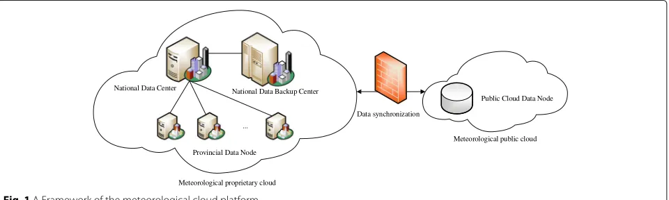
In order to place the big data in the MCP, the structure of the MCP should be figured out. Nowadays, the meteo-rological information system includes the meteometeo-rological database, the meteorological application library, and the meteorological graphic image database [6]. The meteo-rological database is the basis of meteometeo-rological engi-neering, including a huge number of meteorological data. It is mainly responsible for the retrieval of meteorolog-ical information. The meteorologmeteorolog-ical application library mainly carries out mathematical analysis for meteoro-logical elements. In addition, the meteorometeoro-logical graphic image database is responsible for the visual expression and display of meteorological information. Since the acquisition of meteorological data is mainly carried out in meteoro-logical databases, this paper will discuss the distribution of big data on the basis of meteorological databases. Figure1
releases a framework of the MCP in China, which includes a proprietary cloud and a public cloud, and the data processing mainly occurs in the proprietary cloud.
In meteorological cloud platforms, meteorological data are distributed on thousands of physical machines. When a computational task arrives at a physical machine, it may require a variety of meteorological data at different locations for computation. Therefore, this paper uses fat-tree topology structure to construct the meteorological database of MCP [20].
The advantages of the fat-tree structure are obvi-ous. First of all, its bandwidth division increases with the expansion of network scale which can provide high throughput transmission service for MCP. In addi-tion, it can provide communication between different pods. Moreover, there are many parallel paths between source and destination nodes, the fault-tolerant perfor-mance of the network is guaranteed, and there will be no single point of failure in general. Besides, the fat-tree structure achieves timely load handling through multiple links at the core layer, avoiding network hot
National Data Backup Center
Provincial Data Node ... National Data Center
Public Cloud Data Node
Meteorological proprietary cloud
Meteorological public cloud Data synchronization
spots, and avoids overload by reasonable shunting within the pod.
The structure of the fat-tree is mainly composed of three layers of switches which are the core switch, the aggre-gation switch, and the edge switch, and the edge switch is connected with the physical machine. From our former research [21], it can be seen that in the fat-tree topology, every two aggregation switches and two edge switches form a pod. If we figure out the number of pods, the whole network topology is clear. Assuming that the num-ber of the pods in MCP isp, then the number of physical machines that each pod can connect to is(p/2)2, and the number of edge switches and aggregate switches in each pod is p/2; there are (p/2)2 core switches in the whole topology. The number of ports per switch in the network isp, thus the topology can be connected top3/4 physical machines in total.
3 Resource model of MCP
In this section, we construct a resource model of MCP in big data environment based on the fat-tree network topol-ogy structure and establish the multi-objective problem of big data distribution in MCP [22].
3.1 System resource model
In this paper, we focus on a big data-oriented MCP that provides flexible resources for storing meteorologi-cal data. Suppose that there areNmeteorological datasets in the current MCP that need to be placed on the phys-ical machines, denoted as D = {d1,d2,. . .,dN}, andM tasks have arrived at the MCP to be performed, denoted as T = {t1,t2,. . .,tM}. A task may require multiple meteoro-logical datasets to perform, and a meteorometeoro-logical dataset may also be accessed by multiple tasks. Since the num-ber of pods ispin the MCP, thus there arep3/4 physical machines provided to place the datasets and the tasks. Assuming W is the total number of physical machines, W = p3/4, then the physical machines in the MCP can be represented by PM = {pm1,pm2,. . .,pmW}. Hence, setX= {x1,x2,. . .,xN}be the collection of the placement strategy for each meteorological dataset, and each place-ment strategyxn ∈ PM(1 ≤ n ≤ N). Similarly, setY = {y1,y2,. . .,yM} be the collection of the placement loca-tion of each task set, and each placement localoca-tionym ∈ PM(1 ≤ m ≤ M). Therefore, this paper will solve the placement strategyXof meteorological dataset according to the known task placement strategyY. Meteorological data refers to information elements or numerical analy-sis results collected or processed by all possible means of observation, detection, and telemetry, which come from the Earth’s atmosphere and its adjacent layers and are related to the law of atmospheric state change.
According to the types of data in meteorological infor-mation system, meteorological data can be divided into
two categories which are the meteorological data and industrial social data [6]. Meteorological data, includ-ing atmospheric data and surface data, are the main data resources for studying and forecasting meteorologi-cal information, and their data volume is relatively large, while industrial social data mainly include geographic information, national economy and other data, which provide assistance for the analysis of meteorological infor-mation. Because the industrial social data play a restrictive and auxiliary role in meteorological analysis, the indus-trial social data should be placed on the physical machine where the task set is requested, which meansxn = ym. Using binary flag ξn to represent if dn is the industrial social data, thus
ξn=
0,dnis industrial social data,
1, Otherwise. (1)
3.2 Resource utilization model
In MCP, task sets and datasets are managed by virtual machines placed on physical machines. The resources required by datasets and task sets and the capacity of physical machines can be expressed by the number of vir-tual machine instances. Supposecwbe the capacity of the wth physical machinepmw.
Resource utilization is an important metric to manage the utilization of MCP resources. According to the place-ment strategyXof meteorological datasets, the resource utilization of each physical machine can be obtained by detecting the resource utilization of virtual machine instances. Suppose uw(X) be the resource utilization of thewth physical machine under the placement strategyX, which can be calculated by
uw(X)=
whereθnrepresents the resource demand of meteorolog-ical dataset dn, and In,w(X) is the binary flag to judge
Then, the overall resource utilization of MCP refers to the usage status of all occupied physical machines. Sup-poseλ(X)be the number of employed physical machines, which can be calculated by
λ(X)= W
w=1
Fw(X), (4)
whereFw(X) is the binary flag to judge whetherpmwis employed, thus
Fw(X)=
1, pmwis empolyed,
Then, the average resource utilization of the MCP can be obtained by using the following formula
U(X)= 1
3.3 Access time model
In the MCP, the task set needs to be implemented by the meteorological dataset deployed on the physical machine. Hence, when considering the big data distribution strat-egy of meteorological cloud platform, it is necessary to consider the data access time of task set accessing meteo-rological dataset.
Supposelm,nis the binary flag to judge whethertmneeds to accessdn, thus a task execution cycleR, then the total access frequency K in a period of execution cycle can be calculated by the following formula
In the fat-tree topology, the number of exchanges occur-ring in data transmission is closely related to the distribu-tion of datasets and task sets. SupposeES(pm)be the edge switch connected to the physical machines andPod(pm) represents the pod of this edge switch. Then, the num-ber of exchanges in data transmission can be divided into four cases, respectively: (1)tm anddn are placed on the same physical machine, which meansxn=ym. (2)tmand dnare placed on the different physical machines but con-nected to the same edge switch, which meansxn = ym, ES(xn) = ES(ym). (3) The physical machines oftm and dn belongs to different edge switches but the same pod, which meansES(xn) = ES(ym),Pod(xn) = Pod(ym). (4) The physical machines of tm anddn belong to different pods, which means Pod(xn) = Pod(ym). Based on the analysis above, the access timetm,n(X)oftmto accessdn once can be calculated by
tm,n(X)= resents the bandwidth between physical machines and edge switches; similarly, bEA represents the bandwidth between edge switches and aggregation switches andbAC represents the bandwidth between aggregation switches
and the core switches. Then, the average data access time T(X) of the MCP can be calculated using the following formula
3.4 Energy consumption model
In this paper, we focus on the energy consumption of physical machines, virtual machines, and switches in the process of data layout. First of all, all physical machines consume a certain amount of energy to run. We call this energy consumption the basic energy consumption of physical machines, which can be calculated as
BE(X)=
Virtual machine also consumes a certain amount of energy. Its energy consumption can be divided into two situations. If the virtual machine instance is occupied by datasets, it will consume more energy. We call this energy consumption as active virtual machine energy consump-tion, which can be calculated according to the following formula
whereηis the active energy rate of the virtual machines. And the virtual machine instances that are not occu-pied by meteorological datasets will consume less energy, which we call it the idle virtual machine consumption, denoted asIE, can be calculated by
IEVM(X)=
whereτis the idle energy rate of the virtual machines. Therefore, the virtual machine consumption in the MCP can be expressed as
VE(X)=AEVM(X)+IEVM(X). (14)
Hence, the energy consumption of the switchesSEcan be calculated by
SE(X)=5 4p
2·R·β
+ M
m=1 N
n=1
lm,n·gm,n(X)·tm,n(X)·ξn·δm,n(X)·γ,
(16)
whereβis the basic energy rate of the switches andγ is the working energy rate of the switches.
Therefore, the overall energy consumption of meteoro-logical cloud platform can be calculated by
E(X)=BE(X)+VE(X)+SE(X). (17)
3.5 Problem formulation
The focus of our research is to solve the problem of big data placement in the environment of MCP. On the basis of known task set placement strategy, we optimize the placement strategy of meteorological dataset in order to improve resource utilization, reduce data access time and energy consumption.
After the above analysis, the multi-objective problem in this paper can be expressed as
maxU(X), minT(X), minE(X). (18)
s.t.xn= {1, 2,. . .,W}, (19)
N
n=1
θn·In,m(X)≤cw. (20)
4 A big data placement method in MCP
In this section, a data placement method in MCP is proposed. Compared with the other data placement, NSGA-III is widely applied in could platform because of its advantages in finding the optimal solution in the
feasible solution accurately and timely, which is used to MCP in this paper [23,24]. First, the placement strategies for meteorological data sets are encoded and fitness func-tions are given for the optimization problem. Second, the fast non-dominated sorting approach and the crowded-comparison operation are used in selection. Then, the crossover and mutation operation of traditional genetic algorithm (GA) are adopted. Finally, the overview of our method is described in detail.
4.1 Data placement based on NSGA-III
A data placement strategy in MCP is proposed in this subsection. The data placement problem is defined as a multi-objective optimization problem. NSGA-III is an accurate and robust method for addressing the optimiza-tion problem with multiple objectives. Here, NSGA-III is adopted to solve the multi-objective optimization prob-lem presented in [18].
Firstly, we encode for the physical machines and then give the fitness function and constraints for the multi-objective optimization problem. In addition, we gener-ate new chromosomes using the crossover and muta-tion operamuta-tions. At last, we pick out the chromosomes of the next generation, using usual domination principle and reference-point-based selection. The overview of the multi-objective data placement is elaborated.
4.1.1 Encoding
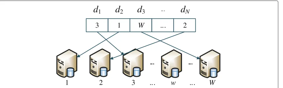
In this section, we encode for the physical machines and meteorological datasets are placed to the physical machines, as is presented in Section 3. In the genetic algo-rithm (GA), a gene represents the data placement strategy of a dataset and the genes compromise a chromosome, representing the placement strategies of all the meteoro-logical datasets. The physical machines are encoded as 1, 2,. . .,W.
Figure2illustrates an encoding instance for placement of the datasets with N meteorological datasets. In this
3
1
W
...
2
d
1
d
2
d
3
...d
N
1
2
3
... ...
w
W
...
...
example, the chromosome is encoded in an array of W integers(1, 2,. . .,W).
4.1.2 Fitness functions and constraints
The fitness functions are adopted to evaluate the solutions generated by the chromosomes. In GA, each chromosome is an individual and represents a solution of the optimiza-tion problem. The fitness funcoptimiza-tions in this paper includes three categories: the average resource utilization, the data access time, and the energy consumption, presented in [6], [10], and [17] respectively. The resource utilization should be maximized and the data access time and the energy consumption must be minimized, and we aim to achieve a balance among those three objectives.
4.1.3 Initialization
In this subsection, the parameters of GA are determined, including the population size S, the maximum itera-tion I, the crossover possibility pc, and the mutation possibilitypm.
Each chromosome represents the placement strategies of all the meteorological datasets, which is denoted asXi =(x1,x2,. . .,xN)(i = 1, 2,. . .,S). Each gene in the chro-mosome stands for the placement strategy of a dataset.
4.1.4 Crossover and mutation
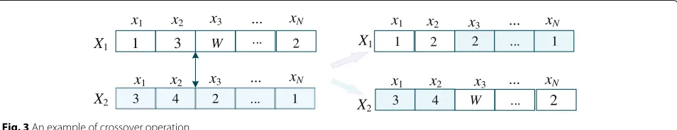
In the crossover phase, we conduct the single-point crossover operation on two chromosomes to generate two new individuals. Figure 3 illustrates an example of crossover operation for two chromosomes withW genes respectively. In this example, a crossover point is deter-mined in advance and then the genes of two chromosomes are swapped around the point. Thus, two new chromo-somes are created.
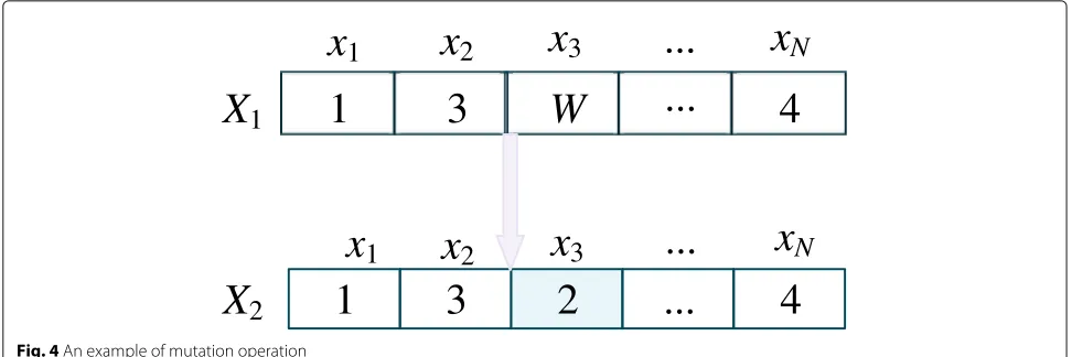
The mutation operation is conducted to modify the genes in chromosomes to create new chromosomes with the hope of higher fitness values. An example of muta-tion operamuta-tion of a chromosome withNgenes is shown in Fig.4. Each gene in the chromosome is changed with the equal possibilitypm.
4.2 Selection for the next generation
We select the chromosomes for the next generation in the selection phase with higher fitness values. We encode for
the physical machines and each chromosome represents all the data placement strategies of the meteorological datasets. As is discussed above, the number of fitness functions for each chromosome is 3, i.e., the resource utilization, the data access time, and the energy con-sumption. After crossover and mutation operations are conducted,Schromosomes are generated and the size of population becomes 2S. We aim at selectSchromosomes for the next generation.
Firstly, the three objectives are evaluated according to [6], [10], and [17]. Then, usual domination principle is conducted to sort the 2Ssolutions using the three fitness values to generate some non-dominated fronts. Suppose that there arennon-dominated fronts, and the datasets in the first front have the most optimal fitness values.
We select one chromosome at random from the first front to the nth fronts every time untilS chromosomes have been picked out. Assume the last chosen solution is in thefth front and the number of the selected chromo-somes in thefth front iss. If the number of solutions in thefth non-dominated front iss, that is all the individu-als in thefth front are selected, then the selection phase finishes.
However, if part of the chromosomes in the fth front are chosen, then further selection is required to determine the chromosomes in the fth front going into the next chromosomes.
In further selection, the three fitness functions of each individual in the generation are normalized. The max-imization of the resource utilization, the minmax-imization of the data access time, and the energy consumption for the population are represented asU∗(X),T∗(X), and E∗(X) respectively. We searchU∗(X),T∗(X), andE∗(X) in the population firstly. Then the fitness functions are updated as
⎧ ⎨ ⎩
U(X)=U(X)−U∗(X), T(X)=T(X)−T∗(X), E(X)=E(X)−E∗(X).
(21)
Um,Tm, and Em represent the extreme values of the average resource utilization, the data access time, and the energy consumption respectively which are calculated by
...
3 4 2 ... 1
2 ... 1
3 4
1
3
... 2 1 22
WW
X
1X
2X
1X
2x
1x
1x
1x
1x
2x
2x
2x
2x
3x
3x
3x
3...
...
...
...
x
Nx
Nx
Nx
N1
3
2
...
4
1
3
W
...
4
X
1
X
2
x
1
x
1
x
2
x
2
x
3
x
3
...
...
x
N
x
N
Fig. 4An example of mutation operation
⎧ ⎪ ⎨ ⎪ ⎩
Um=maxU
(X)
WU , Tm=maxT
(X)
WT , Em=maxE
(X)
WE ,
(22)
whereWU,WT, andWEare the weight vectors to the three functions.
Assume each fitness function as an axis and the inter-cepts of each axis can be determined according to the three extreme values, denoted asρU,ρT, andρE respec-tively. Then, the fitness functions are normalized by
= ⎧ ⎪ ⎨ ⎪ ⎩
U(X)= Uρ(X) U , T(X)= Tρ(X)
T , E(X)= Eρ(X)
E .
(23)
After normalization, the fitness values of the resource utilization, the data access time, and the energy consump-tion are between zero and one. The normalized soluconsump-tions are scattered in the hyperplane composed by the three fit-ness axes. Each solution of the individual in the population is corresponding to a triple.
Divide each axis intogsubsections, and then, the num-ber of the reference points, denoted asζ, is calculated by
ζ =Cgg+2. (24)
ζis approximately equal toSto guarantee each individual associate with a reference point. Then, we associate the normalized solutions with the reference points.
We sort the solutions in thefth non-dominated front, using the number of the associated reference points. Assume the solutions in thefth front are sorted intod lev-els and the reference points in the first level represents the maximum reference points. Each time selects one solution randomly from the first level until thenindividuals have been selected.
4.3 Solution evaluation using SAW and MCDM
The proposed strategy aims at achieving a trade-off in optimizing the average resource utilization, the data access time of the tasks, and the energy consumption of MCP. In each population, there areN chromosomes and each chromosomexnrepresents a hybrid data placement ofNmeteorological datasets. In addition, dynamic sched-ule of datasets is considered and, to select relatively bet-ter schedule solution of each placement strategy, simple additive weighting (SAW) and multiple criteria decision making (MCDM) are employed.
The resource utilization is a positive criterion, i.e., the higher the resource utilization is, the better the solution becomes. Oppositely, the data access time and the energy consumption are the negative criterion. We normalize the resource utilization in thenth placement strategy as
UV(Un)=
U(xn)−Umin
Umax−Umin,Umax−Umin=0,
1,Umax−Umin=0, (25)
whereUmaxandUminrepresent the maximum and mini-mum fitness for resource utilization in thenth placement strategy. Similarly, the time consumption ofnth placement strategy is normalized as
UV(Tn)=
Tmax−T(xn)
Tmax−Tmin,Tmax−Tmin=0,
1,Tmax−Tmin=0, (26)
whereTmaxandTminrepresent the maximum and min-imum fitness for data access time in the nth placement strategy. And the energy consumption ofnth placement strategy is normalized as
UV(En)=
Emax−E(xn)
Emax−Emin,Emax−Emin=0,
1,Emax−Emin=0, (27)
solution, the weight of each objective function requires determination.
In this paper, we do an overall consideration of three objectives for each strategy. The utility value of thenth placement strategy is calculated by
UV(xn)=UV(Un)·κU+UV(Tn)·κT+UV(En)·κE, (28)
where UV(xn) represents the utility value of the nth placement strategy and κU, κT, and κE represent the weight of the resource utilization, the data access time, and the energy consumption respectively. Therefore, for each chromosome in the population, we have calculated the utility value of the same schedule. The formalized optimization problem given in (18) can be represent by
N max
n=1UV(xn) (29)
s.t.xn= {1, 2,. . .,W}, (30)
N
n=1
θn·In,m(X)≤cw, (31)
κU,κT,κE ∈[ 0, 1] , (32)
κU+κT+κE=1. (33)
The solution selection strategy is elaborated in Algorithm 1. We select the maximum and minimum value of the three objections (Lines 1-6). Then the utility values of the three objections and the solutions are evalu-ated (Lines 7-12). The maximum utility value of solution is selected (Line 13). Finally, the solution with maximum utility value is output.
Algorithm 1Solution evaluation Require: κU,κT,κE,X
Ensure: UV n=1
whilen≤Ndo
3: Evaluate the fitness functions by (6), (10) and (17)
n=n+1 end while
6: Select the maximum and minimumU(X),T(X),E(X) N=1
whilen≤Ndo
9: Evaluate the utility value ofU(X),T(X),E(X)in (25-27)
Evaluate the utility value ofn-th placement strat-egy in (28)
n=n+1
12: end while
Select the maximum utility valueUV returnUV
4.4 Method overview
In this paper, we aim to optimize the resource utilization, reduce the data access time, and decrease the energy con-sumption, which is determined as a multi-objective opti-mization problem. The NSGA-III is adopted to achieve the global optimal data placement strategy. First, we encode for the physical machines and each gene rep-resents the data placement strategy for a meteorologi-cal dataset. Then, the fitness functions and constraints of the multi-objective optimization problem are elabo-rated. Crossover and mutation operations are conducted to generate new chromosomes and usual domination principle and reference-point-based selection in NSGA-III are adopted to select the individuals going into the next generation.
The overview of the proposed method is elaborated in Algorithm 2. We input the tasks, the physical machines, and the placement strategy of the tasks. The algorithm starts with the first iteration, and for each iteration, we conduct the crossover and mutation operation to gener-ate new solutions (Line 3). Then, we evalugener-ate the fitness functions of each chromosomes and obtain the placement routing (Lines 5). We conduct the selection, including the non-dominant sorting, the primary selection, and the fur-ther selection (Lines 7-13). When the algorithm reaches
Algorithm 2Data Placement method in MCP Require: PM,T,Y,X.
Ensure: X∗ i=1
whilei≤Ido
3: Crossover and mutation operation forthe individuals in the populationdo
Evaluate the fitness functions by (6), (10) and (17)
6: end for
Non-dominant sorting the individuals
Primarily select the solutions from the first front
9: if part of solutions in thef-th front are selected
then
Normalize the solutions by (21-23)
Generate the reference points with the con-straints (24)
12: Associate the reference points with the nor-malized solutions off-th front
Select the solutions with the maximum associ-ated reference points
end if
15: i=i+1
end while
Evaluate the solutions in the last iteration according toAlgorithm 1
the maximum iteration, we evaluate the solutions by SAW and MCDM (Line 17). Finally, the optimal data placement methods are output.
5 Experimental evaluation
In this section, a set of complex simulations and exper-iments are performed to evaluate the performance of the proposed DPMM. We first introduced the simula-tion setup with the simulasimula-tion parameter settings and the statement of the comparative data placement. Then, the influence of different task scales on the performance of the resource utilization, the data access time, and the energy consumption of the compared method and our proposed DPMM is evaluated.
5.1 Simulation setup
In our simulation, six datasets with different scales of the tasks are applied for our experiments, and the number of datasets is set to 200, 400, 600, 800, 1000, and 1200 and the industrial social datasets is set to 50, 100, 150, 200, 250, and 300 in each scale of the meteorological datasets. The specified parameter settings in this experiment are illustrated in Table1[25].
To conduct the comparison analysis, we employ some other basic data placement method besides our DPMM. The comparative methods are briefly expounded as fol-lows:
• Benchmark: In this method, the meteorological datasets are placed in the order of the physical machines. When the former physical machine is full, the datasets left are placed on the next physical machine. This process is repeated until all datasets have been placed.
•First fit decreasing in MCP (FFD-M): The meteoro-logical datasets are sorted in descending order according to the dataset requests first. Then, the sorted datasets are
Table 1Parameter settings
Parameter description Value
The number of tasksM 40
The time of running periodR 24 h
The number of physical machinesW 2000
The baseline energy consumption rate of wth physical machineαw
342 W
The active energy consumption rate for each virtual machineη
37 W
The bandwidth between severs and edge switchesbSE
50 M
The bandwidth between switches in the fat-tree topologybEAandbAC
100 M
The idle energy consumption rate for each switchβ
100 W
The active energy consumption rate for each switchγ
150 W
placed on the physical machines. If the left resources of current physical machine are insufficient for the resource requirement of a dataset, the dataset is placed on the physical machine with enough resource. This process is repeated until all datasets have been placed.
•Best fit decreasing in MCP (BFD-M): The meteorolog-ical datasets and the physmeteorolog-ical machines are both sorted in descending order according to the dataset request and the space of physical machines first. Then, the sorted datasets are placed on the sorted physical machines. If the left resources of the physical machine are insufficient for the resource requirement of the dataset, the dataset is placed on the physical machine with enough resource next to this physical machine in optimal principle. This process is repeated until all datasets have been placed.
The data placement methods are implemented on a personal computer with Intel Core i7-4720HQ 3.60 GHz processors and 4 GB RAM.
5.2 Performance evaluation of DPMM
The proposed DPMM is intended to achieve a trade-off with optimizing the resource utilization while reducing the data access time and the energy consumption. We con-ducted 50 experiments in the case of convergence for each dataset scale, and multiple sets of results are obtained.
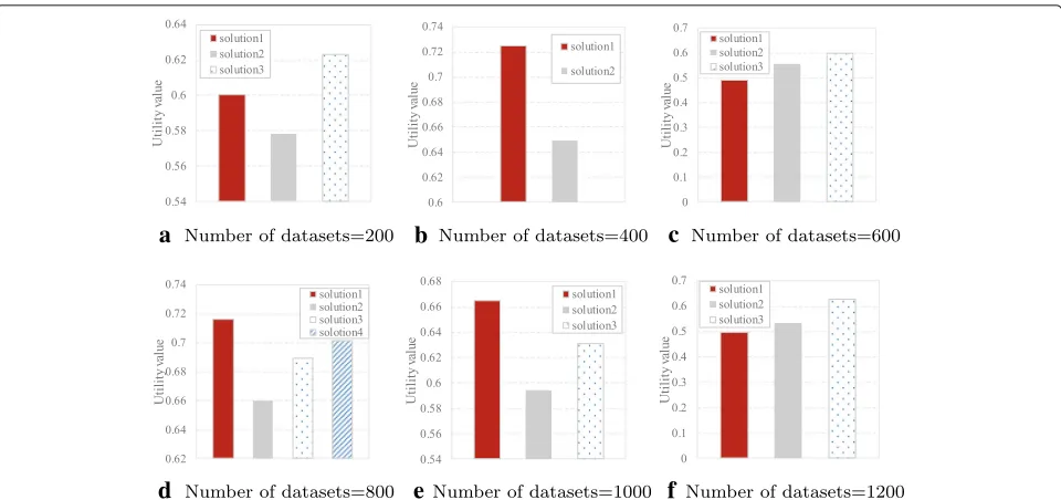
Figure5shows the comparison of the utility value of the solutions generated by DPMM at different dataset scales. It is illustrated that when the dataset scale is 200, 400, 600, 800, 1000, and 1200, solutions generated by DPMM are 3, 2, 3, 4, 3, and 3 respectively. For the solutions gener-ated by DPMM, we attempt to obtain the most balanced data placement strategy by judging the utility value given in [28]. After statistics and analysis, the solution with the maximum utility value is considered as the most balanced strategy. For instance, in Fig.5a, the final selected strategy is solution 3 because it achieves the highest utility value.
5.3 Comparison analysis
In this subsection, the comparisons of Benchmark, FFD-M, BFD-FFD-M, and DPMM with the same experimental con-text are analyzed in detail. The resource utilization, the data access time, and the energy consumption are the main metrics for evaluating the performance of the data placement method. The corresponding results are shown in Figs.6,7, and8.
a
b
c
d
e
f
Fig. 5Comparison of the utility value of the solutions generated by DPMM at different data scales.aNumber of datasets = 200.bNumber of datasets = 400.cNumber of datasets = 600.dNumber of datasets = 800.eNumber of datasets = 1000.fNumber of datasets = 1200
physical machines with more occupied VM instances con-tribute to a higher resource utilization. It is intuitive from Fig.6that our proposed method DPMM achieves higher and stable resource utilization. That is, DPMM reduces the number of unemployed VM instances and wastes less resources than other data placement method.
(2) Comparison of data access time: Fig. 7 shows the comparison of the data access time of the meteorologi-cal tasks of Benchmark, FFD-M, BFD-M, and DPMM at different dataset scales. In this paper, we try to realize a balance between the resource utilization, the data access time and the energy consumption; however, in order to improve the resource utilization and reduce the energy
consumption, the meteorological datasets may place on the physical machine which may be far from the tasks. It is illustrated from Fig. 7 that the data access time of our proposed method DPMM is a little more than the other data placement method, which means our proposed method may sacrifice some data access time to optimize the resource utilization and the energy consumption.
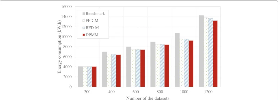
(3) Comparison of energy consumption: As the energy consumption is the sign of the cost the MCP needs to give out, it becomes the most important metrics that the manager of the MCP concerned. Figure8shows the com-parison of energy consumption in MCP of Benchmark, FFD-M, BFD-M, and DPMM at different dataset scales.
0 10 20 30 40 50 60 70 80 90 100
200 400 600 800 1000 1200
Resource utilization
(%)
Number of the datasets
Benchmark FFD-M BFD-M DPMM
0 100 200 300 400 500 600 700 800 900 1000
200 400 600 800 1000 1200
Data access tim
e
(m
s)
Number of the datasets
Benchmark FFD-M BFD-M DPMM
Fig. 7Comparison of the data access time of the meteorological tasks of Benchmark, FFD-M, BFD-M, and DPMM at different dataset scales
When the number of the datasets is small, the difference of the energy consumption for those four data placement methods are not obvious, but with the increase of the dataset scales, the energy consumption of DPMM is bet-ter than the other data placement method, which means that our proposed method DPMM may well be applied in the big data environment like MCP.
6 Related work
In recent years, with the rapid growth of meteorological data resources, people are actively seeking to replace the traditional meteorological information system platform, and the MCP has attracted extensive attention because of its high-efficiency computing ability for large data [26,27]. Pokric et al. [6] presents the environmental itoring solution ekoNET, developed for a real-time mon-itoring of air pollution and other atmospheric condition
parameters such as temperature, air pressure, and humid-ity. In [28], Sawant et al. addresses above issues through the adaptation of a framework based on Open Geospa-tial Consortium standards for Sensor Web Enablement. Padarian et al. in [29] explores the feasibility of using this platform for digital soil mapping by presenting two soil mapping examples over the contiguous USA.
However, with the increasing amount of data, the prob-lem of data placement in meteorological cloud data center is becoming more and more serious [30,31]. Traditional data placement method cannot meet the basic require-ments of query and analysis of massive data. A new data placement method for big data needs to be applied to MCP immediately [32]. The data placement method has been widely researched in many studies [33]. In [34], Yu and Pan proposed an associated data placement scheme, which improves the co-location of associated data and the
0 2000 4000 6000 8000 10000 12000 14000 16000
200 400 600 800 1000 1200
Energy consum
ption (kW
.h)
Number of the datasets
Benchmark FFD-M BFD-M DPMM
localized data serving while ensuring the balance between nodes. In [35], Paiva et al. addressed the problem of self-tuning the data placement in replicated key-value stores to automatically optimize replica placement in a way that leverages locality patterns in data accesses, such that internode communication is minimized.
In the study of data placement methods, a large num-ber of methods such as operations research are applied to optimize them [36,37]. And a large number of studies such as [38–41] and [42] are carried out. Compared with these methods, genetic algorithms have more rapid and accurate characteristics, and better adapt to the require-ments of data placement in big data environment. Many studies focus on genetic algorithms [43].
In [44], Jean-Luc et al. compared genetic algorithm to a pure random optimization approach and their optimiza-tion efficiencies are analyzed. In [45], Kadri and Boctor addressed the resource-constrained project scheduling problem with transfer times and the experiment, con-ducted on a large number of instances, shows that the proposed algorithm performs better than several solution methods previously published. In [46], a set-based Pareto dominance relation was then defined to modify the fast non-dominated sorting approach in NSGA-II.
However, with the observation above, few studies have been conducted about the data placement in MCP facing with the big data. In this paper, we employed one of the genetic algorithm NSGA-III to optimize the resource uti-lization, the data access time, and the energy consumption in MCP.
7 Conclusion and future work
The existing works of meteorological data placement in MCP have not combined the energy consumption and the data access time together. In this paper, a big data place-ment method in MCP is proposed. We construct as sys-tematic model of the resource utilization, the data access time, and the energy consumption in MCP. The proposed method is designed to improve the average resource uti-lization in MCP and access performance while reducing the energy consumption using the NSGA-III. Through adequate experimental evaluation and comparison anal-ysis, the efficiency and effectiveness of our proposed method are validated.
For future work, we will adjust and extend our method to implement the meteorological data placement in exact physical environment. Accordingly, the data access time should also be reduced than the result of this paper in future.
Acknowledgements
This work is supported by The Startup Foundation for Introducing Talent of NUIST, the open project from State Key Laboratory for Novel Software Technology, Nanjing University under grant no. KFKT2017B04, the Priority Academic Program Development of Jiangsu Higher Education Institutions
(PAPD) fund, Jiangsu Collaborative Innovation Center on Atmospheric Environment and Equipment Technology (CICAEET), and the project “Six Talent Peaks Project in Jiangsu Province” under grant no. XYDXXJS-040.
Funding
This research is supported by the National Science Foundation of China under grant no. 61702277, no. 61872219, and no. 61772283 with the help of data collection and analysis.
Availability of the data and materials
The dataset employed to support the conclusion of this article is available at http://data.cma.cn/.
Authors’ contributions
FR, RG, and TH conceived and designed the study. RG and TH performed the simulations. FR and RG wrote the paper. All authors reviewed and edited the manuscript. All authors read and approved the final manuscript.
Authors’ information
Not applicable.
Competing interests
The authors declare that they have no competing interests.
Publisher’s Note
Springer Nature remains neutral with regard to jurisdictional claims in published maps and institutional affiliations.
Author details
1School of Automation, Nanjing University of Information Science &
Technology, Nanjing, China.2School of Computer and Software, Nanjing University of Information Science and Technology, Nanjing, China.3Jiangsu
Engineering Center of Network Monitoring, Nanjing University of Information Science and Technology, Nanjing, China.4School of Computer Science and
Technology, Silicon Lake College, Suzhou, China.
Received: 15 March 2019 Accepted: 25 April 2019
References
1. A. Stein, R. R. Draxler, G. D. Rolph, B. J. Stunder, M. Cohen, F. Ngan, NOAA?s HYSPLIT atmospheric transport and dispersion modeling system. Bull. Am. Meteorol. Soc.96(12), 2059 (2015)
2. A. T. Eseye, J. Zhang, D. Zheng, Short-term photovoltaic solar power forecasting using a hybrid Wavelet-PSO-SVM model based on SCADA and Meteorological information. Renew. Energy.118, 357 (2018)
3. S. Fan, J. R. Liao, R. Yokoyama, L. Chen, W. J. Lee, Forecasting the wind generation using a two-stage network based on meteorological information. IEEE Trans. Energy Convers.24(2), 474 (2009) 4. V. S. Sherstnyov, A. I. Sherstnyova, I. A. Botygin, D. A. Kustov, inKey
Engineering Materials, vol. 685. Distributed information system for processing and storage of meteorological data (Trans Tech Publ, Boston, 2016), pp. 867–871
5. J. Brenton, Status of the Meteorological Data Format Working Group (2016).https://ntrs.nasa.gov/search.jsp?R=20160011066. Accessed 13 May 6. B. Pokric, S. Kreo, D. Drajic, M. Pokric, I. Jokic, M. J. Stojanovic, in2014 Eighth
International Conference on Innovative Mobile and Internet Services in Ubiquitous Computing. ekoNET-environmental monitoring using low-cost sensors for detecting gases, particulate matter, and meteorological parameters (IEEE Computer Society, Washington, DC, 2014), pp. 421–426 7. J. Elston, B. Argrow, M. Stachura, D. Weibel, D. Lawrence, D. Pope,
Overview of small fixed-wing unmanned aircraft for meteorological sampling. J. Atmos. Ocean. Technol.32(1), 97 (2015)
8. X. Xu, Y. Li, T. Huang, Y. Xue, K. Peng, L. Qi, W. Dou, An energy-aware computation offloading method for smart edge computing in wireless metropolitan area networks. J. Netw. Comput. Appl.133, 75–85 (2019) 9. J. Figa-Saldaña, J. J. Wilson, E. Attema, R. Gelsthorpe, M. Drinkwater, A.
10. https://www.nice-software.com/solutions/cloud-computing. Accessed 3 Feb 2019
11. X. Wang, L. T. Yang, L. Kuang, X. Liu, Q. Zhang, M. J. Deen, A Tensor-Based Big-Data-Driven Routing Recommendation Approach for Heterogeneous Networks. IEEE Netw.33(1), 64 (2018)
12. S. Wang, A. Zhou, M. Yang, L. Sun, C. H. Hsu, Service composition in cyber-physical-social systems. IEEE Trans. Emerg. Top. Comput. (2017). https://doi.org/10.1109/TETC.2017.2675479
13. X. Xu, Q. Liu, Y. Luo, G. Xing, K. Peng, Z. Xu, S. Meng, L. Qi, A Computation Offloading Method over Big Data for IoT-Enabled Cloud-Edge Computing, Future Generation Computer Systems. Futur. Gener. Comput. Syst.95, 522–533 (2018)
14. Y. Xu, L. Qi, W. Dou, J. Yu, Privacy-preserving and scalable service recommendation based on simhash in a distributed cloud environment. Complexity.2017, 1–9 (2017)
15. X. Wang, L. T. Yang, X. Xie, J. Jin, M. J. Deen, A cloud-edge computing framework for cyber-physical-social services. IEEE Commun. Mag.55(11), 80 (2017)
16. X. Xu, Y. Xue, L. Qi, Y. Yuan, X. Zhang, T. Umer, S. Wan, An edge computing-enabled computation offloading method with privacy preservation for internet of connected vehicles. Futur. Gener. Comput. Syst.96, 89–100 (2019) 17. X. Xu, X. Zhang, M. Khan, W. Dou, S. Xue, S. Yu, A Balanced Virtual Machine Scheduling Method for Energy-Performance Trade-offs in Cyber-Physical Cloud Systems. Futur. Gener. Comput. Syst.18, 1–11 (2017)
18. S. Wang, A. Zhou, R. Bao, W. Chou, S. Yau, Towards Green Service Composition Approach in the Cloud. IEEE Trans. Serv. Comput. (2018). https://doi.org/10.1109/TSC.2018.2868356
19. L. Ren, X. Cheng, X. Wang, J. Cui, L. Zhang, Multi-scale Dense Gate Recurrent Unit Networks for bearing remaining useful life prediction. Futur. Gener. Comput. Syst.94, 601 (2019)
20. N. Jain, A. Bhatele, L. H. Howell, D. Böhme, I. Karlin, E. A. León, M. Mubarak, N. Wolfe, T. Gamblin, M. L. Leininger, inProceedings of the International Conference for High Performance Computing, Networking, Storage and Analysis. Predicting the performance impact of different fat-tree configurations (IEEE Computer Society, Washington, DC, 2017), p. 50 21. X. Xu, S. Fu, L. Qi, X. Zhang, Q. Liu, Q. He, S. Li, An IoT-oriented data
placement method with privacy preservation in cloud environment. J. Netw. Comput. Appl.124, 148 (2018)
22. X. Xu, X. Zhao, F. Ruan, J. Zhang, W. Tian, W. Dou, A. Liu, Data Placement for Privacy-Aware Applications over Big Data in Hybrid Clouds. Secur. Commun. Networks.2017, 1–15 (2017)
23. G. Wang, X. Huang, J. Zhang, Levitin–Polyak well-posedness in generalized equilibrium problems with functional constraints. Pac. J. Optim.6, 441 (2010)
24. W. Gang, H. Xuexiang, Z. Jie, C. Guangya, Levitin-poyak well-posedness of generalized vector equilibrium problems with functional constraints. Acta Math. Sci.30(5), 1400 (2010)
25. http://data.cma.cn/. Accessed 26 Jan 2019
26. K. Bessho, K. Date, M. Hayashi, A. Ikeda, T. Imai, H. Inoue, Y. Kumagai, T. Miyakawa, H. Murata, T. Ohno, et al., An introduction to
Himawari-8/9—Japan’s new-generation geostationary meteorological satellites. J. Meteorol. Soc. Jpn. Ser. II.94(2), 151 (2016)
27. E. Gordeev, O. Girina, E. Lupyan, A. Sorokin, L. Kramareva, V. Y. Efremov, A. Kashnitskii, I. Uvarov, M. Burtsev, I. Romanova, et al., The VolSatView information system for Monitoring the Volcanic Activity in Kamchatka and on the Kuril Islands. J. Volcanol. Seismol.10(6), 382 (2016)
28. S. Sawant, S. S. Durbha, A. Jagarlapudi, Interoperable agro-meteorological observation and analysis platform for precision agriculture: A case study in citrus crop water requirement estimation. Comput. Electron. Agric.
138, 175 (2017)
29. J. Padarian, B. Minasny, A. B. McBratney, Using Google’s cloud-based platform for digital soil mapping. Comput. Geosci.83, 80 (2015) 30. K. Yumimoto, T. Nagao, M. Kikuchi, T. Sekiyama, H. Murakami, T. Tanaka, A.
Ogi, H. Irie, P. Khatri, H. Okumura, et al., Aerosol data assimilation using data from Himawari-8, a next-generation geostationary meteorological satellite. Geophys. Res. Lett.43(11), 5886 (2016)
31. M. B. Hahn, A. J. Monaghan, M. H. Hayden, R. J. Eisen, M. J. Delorey, N. P. Lindsey, R. S. Nasci, M. Fischer, Meteorological conditions associated with increased incidence of West Nile virus disease in the United States, 2004–2012. Am. J. Trop. Med. Hyg.92(5), 1013 (2015)
32. S. Ansari, S. Del Greco, E. Kearns, O. Brown, S. Wilkins, M. Ramamurthy, J. Weber, R. May, J. Sundwall, J. Layton, et al., Unlocking the potential of
NEXRAD data through NOAA’s Big Data Partnership. Bull. Am. Meteorol. Soc.99(1), 189 (2018)
33. J. C. Anjos, I. Carrera, W. Kolberg, A. L. Tibola, L. B. Arantes, C. R. Geyer, MRA++: Scheduling and data placement on MapReduce for
heterogeneous environments. Futur. Gener. Comput. Syst.42, 22 (2015) 34. B. Yu, J. Pan, in2015 IEEE Conference on Computer Communications
(INFOCOM). Location-aware associated data placement for geo-distributed data-intensive applications (IEEE Computer Society, Washington, DC, 2015), pp. 603–611
35. J. Paiva, P. Ruivo, P. Romano, L. Rodrigues, P. A uto, lacer: Scalable Self-Tuning Data Placement in Distributed Key-Value Stores. ACM Trans. Auton. Adapt. Syst. (TAAS).9(4), 19 (2015)
36. H. Chen, Y. Wang, A new CQ method for solving split feasibility problem. Appl. Math. Comput.218(8), 4012 (2011)
37. H. Zhang, Y. Wang, A family of higher-order convergent iterative methods for computing the Moore–Penrose inverse. Front. Math. China.5(1), 37 (2010)
38. C. Hou, W. Yuan, The convergence of conjugate gradient method with nonmonotone line search. Math. Ann.353(2), 499 (2012)
39. G. Wang, H. t. Che, H. b. Chen, Feasibility-solvbility theorems for generalized vector equilibrium problem in reflexive banach spaces. fixed point theory appl.2012(1), 38 (2012)
40. C. Hou, H. Zhang, Derivations of a class of Kadison–Singer algebras. Linear Algebra Appl.436(7), 2406 (2012)
41. Z. J. Shi, S. Wang, Z. Xu, Minimal generating reflexive lattices of projections in finite von Neumann algebras. Mathematische Annalen.
353(2), 499–517 (2012)
42. C. Hou, Minimal generating reflexive lattices of projections in finite von Neumann algebras. Linear Algebra Appl.466, 241 (2015)
43. L. Huan, B. Qu, J. g. Jiang, Merit functions for general mixed
quasi-variational inequalities. J. Appl. Math. Comput.33(1-2), 411 (2010) 44. R. Jean-Luc, F. Gonon, L. Favre, E. L. Niederhäuser, in2018 International
Conference on Smart Grid and Clean Energy Technologies (ICSGCE). Convergence of Multi-Criteria Optimization of a Building Energetic Resources by Genetic Algorithm (IEEE Computer Society, Washington, DC, 2018), pp. 150–155
45. R. L. Kadri, F. F. Boctor, An efficient genetic algorithm to solve the resource-constrained project scheduling problem with transfer times: The single mode case. Eur. J. Oper. Res.265(2), 454 (2018)