A WSN positioning algorithm based on 3D discrete chaotic mapping

R E S E A R C H

Open Access

A WSN positioning algorithm based on 3D

discrete chaotic mapping

Tu Li

, Wang Yan

, Li Ping

and Peng Fang

Abstract

Wireless sensor networks are featured by restricted network resources, which is quite possible to result in low positioning precision and serious time delay in positioning, accordingly, the overall network positioning quality may be reduced; to improve the positioning precision of WSN, based on the DV-HOP positioning algorithm, two aspects of the node positioning were improved from the error precision and least square estimation; thus, a WSN positioning algorithm based on 3D discrete chaotic mapping was proposed: first, a 3D discrete chaotic mapping was constructed, the Chaos Optimization Algorithm was introduced into the positioning error precision calculation, and the unknown nodes were positioned by introducing the least square estimation; second, a simulation experiment of new algorithm was performed from the aspects of communication radius and topological structure. The experimental results showed that the algorithm proposed in this paper can effectively reduce the positioning error caused by calculation and improved the positioning precision. Further, based on the algorithm of this paper, the moving mechanism could be introduced to make dynamic planning for overall network resources, so that the energy cost of the algorithm of this paper in the confirmation process of WSN network terminal could be further reduced to make the algorithm more valuable in engineering field.

Keywords:Wireless sensor networks, Node positioning, Chaos optimization, Least squares estimation

1 Introduction

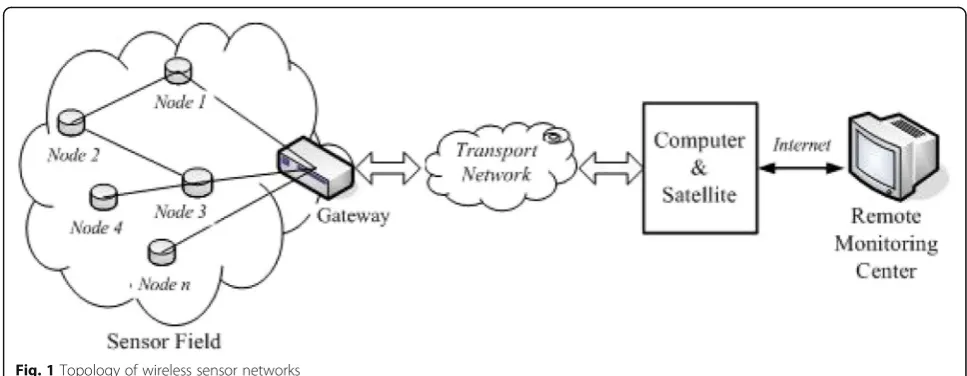
With the development of electronic technology and Inter-net communication technology, the cost of collecting and processing multimedia information (such as images and audio) is getting lower and lower, and the scalar informa-tion collected by tradiinforma-tional sensor networks (such as temperature, humidity, pressure) becomes unable to satisfy the diversified application of the information, therefore, the wireless sensor networks (WSN) emerged [1–7]. Fea-tured by low-cost, rapid network establishment, dynamic topology, and multi-hop routing, WSN is widely applied in industries such as environmental monitoring and industrial technology. WSN integrates the sensor technology, em-bedded computing technology, modern network technol-ogy, and wireless communication technique and is able to perform the real-time monitoring and collection of moni-toring objects information through various microsensors. The information is sent in a wireless way and transmitted to user terminal through ad hoc and multi-hop network,

so as to achieve the targeted information acquisition [8,9]. A typical network topology is shown in Fig.1.

WSN is a hop network composed of micro multi-media sensor nodes which are interlinked and battery

powered. From Fig. 1, it can be found that each sensor

node is able to process the multimedia data for being equipped with wireless transceiver module, and the vol-ume, power dissipation, operation and storage capability, and wireless communication distance of the nodes are all available to be customized based on application needs. The network nodes in WSN are randomly distributed, with the control center node, without fixed organization structure; ad hoc networks are conducted by information interaction and intercoordination of nodes in networks [9, 10]. The sensor nodes are set in site to observe the phys-ical phenomenon; in most cases, only the data included position information is of practical significance; therefore, the node positioning technology plays a very important role in WSN system.

© The Author(s). 2019Open AccessThis article is distributed under the terms of the Creative Commons Attribution 4.0 International License (http://creativecommons.org/licenses/by/4.0/), which permits unrestricted use, distribution, and reproduction in any medium, provided you give appropriate credit to the original author(s) and the source, provide a link to the Creative Commons license, and indicate if changes were made.

* Correspondence:[email protected]

2_{School of Information and Electronic Engineering, Hunan City University,} Yiyang, China

2 WSN node positioning methods

The node positioning system includes distance meas-urement, position calculation, and positioning algo-rithm which are explained below respectively:

1. Distance (angle) measurement: information on the distance (angle) between nodes is acquired by physical distance measurement or multi-hop links; 2. Position estimation: the unknown nodes’position

can be estimated through the information on the distance (angle). If there are anchor nodes, the unknown nodes’position can be estimated through calculation;

3. Positioning algorithm: selecting right positioning algorithm according to the WSN application site. The position of all unknown nodes within the monitored area can be acquired through positioning algorithm on the basis of previous information.

2.1 Computing methods of WSN node positioning

The computing methods of WSN node positioning are divided three classes: trilateration [11], angular

meas-urement [12], and maximum likelihood method [13,

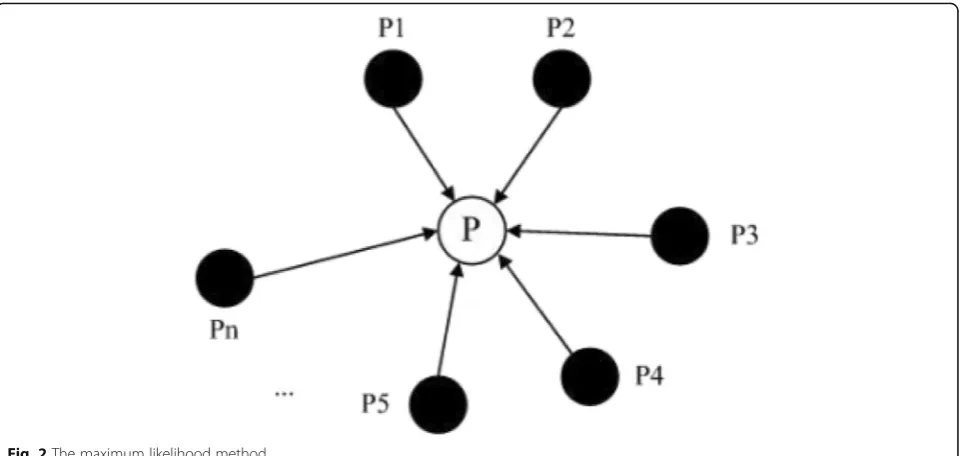
14]. The maximum likelihood method is also named

multilateral measurement, when the data satisfy the Gaussian distribution, it is equal to the least square method. To solve the overdetermined equation, the maximum likelihood method needs the known anchor

nodes ofn coordinates position to calculate the

coord-inate position of the positioned node. The principles of maximum likelihood method are presented below:

Assuming that the measured distance between the positioned nodep(x,y) and the anchor nodes within the measuring radius p1(x1,y1), p2(x2,y2), …, pn(xn,yn) are

d1, d2, d3..., respectively, the following Eq. (1) can be

obtained from the distance formula between two points:

Equation (2) can be obtained by subtracting the n-1th equation fromnth equation in proper order:

xn

can be obtained by using the least mean square error. Compared with the trilateration, the maximum likeli-hood method has higher positioning precision, and with superfluous term, the fault freedom is excellent.

The maximum likehood is shown in Fig. 2.

2.2 WSN node positioning algorithms

The WSN node positioning algorithms are divided in the following classes:

1. Positioning algorithms based on and regardless of distance measurement

The range-based positioning algorithm calculates the node position by measuring the distance between nodes or the angle information and mainly includes the received signal strength indicator-based algorithm (RSSI) [15], time of advent-based positioning algorithm (TOA) [16], time difference of advent-based positioning

algorithm (TDOA) [17], and angle of advent-based

po-sitioning algorithm (AOA) [18]. These algorithms are

featured by higher precision, higher requirements on hardware, higher cost, and being limited by distance measurement technology.

The positioning algorithms regardless of distance meas-urement acquire the distance between nodes through the fixed multi-hop communication relationship of WSN [19], so as to calculate the position of positioned node. They are featured by low cost and easy realization and are suitable for site with dense nodes.

2. Incremental positioning algorithms and concurrent positioning algorithms

The incremental positioning algorithms take the anchor node as core point, starting from the neighbor nodes of an-chor node, to expand outwards. The node positioning are conducted one-by-one by choosing the correct computing method according to the distance between the positioned node and known node or the angle information; in current positioning algorithms, all the unknown nodes confirm their position based on the coordinate information of an-chor node’s position without order. In incremental posi-tioning algorithms, the errors accumulate gradually, which results in lower and lower positioning precision; therefore, it is suitable for the sensor network where there are many nodes and little anchor nodes and with wide coverage area.

3. Positioning algorithms based on anchor node and positioning algorithms without anchor node

While using the positioning algorithms based on anchor node, the anchor node is taken as a reference, through cor-responding positioning calculation, and the unknown nodes are able to acquire their position coordinate; while using the positioning algorithms without anchor node, the anchor node is not involved in positioning, but the relative coordinates of nodes are necessary to be confirmed. Next, the relative coordinates are combined to establish the sys-tem and the unknown nodes will have an overall relative coordinates after the positioning process ended.

2.3 DV-HOP algorithm

Distance vector (DV)-HOP algorithm means to express the distance between the anchor node and unknown nodes with the product of hop count and the average distance between hops [20]. The detailed steps are de-scribed below:

1. Storing the average hop count from anchor node acquired by all unknown nodes;

2. Calculating the average value of hop distance of each anchor node and transmitting to network;

Hij¼ X

i≠j

ffiffiffiffiffiffiffiffiffiffiffiffiffiffiffiffiffiffiffiffiffiffiffiffiffiffiffiffiffiffiffiffiffiffiffiffiffiffiffiffi xi−xj

2

þ yi−yj 2

r

X

i≠j

cij

ð3Þ

In Eq. (3), (xi,yi) and (xj,yj) represent the coordinates of anchor nodes i and j, respectively, and cij is the hop count between anchor nodesiandj.

3. According to the principle that three points determine a plane, the unknown nodes need the hop distance of at least n (n> 3) anchor nodes to acquire the coordinates of their position.

ffiffiffiffiffiffiffiffiffiffiffiffiffiffiffiffiffiffiffiffiffiffiffiffiffiffiffiffiffiffiffiffiffiffiffiffi

There are two problems existing in the traditional DV-HOP algorithm, one is the error which occurred in the calculation of the average hop distance, and the other is the larger error of average hop distance while replacing the unknown nodes with anchor nodes.

3 Improved DV-HOP algorithm

In this paper, the average hop distance of the whole net-work in literature [19] is firstly used to replace the

ori-ginal average hop distance, where n is the number of

anchor nodes in the network, as shown in Eq. (5):

Fi¼ P

Hij

n ð5Þ

The error in hop distance of the whole network is

ac-quired by using Eq. (5) to calculate the average hop

distance of the whole network, as shown in Eq. (6):

f ¼

where the numerator represents the difference of the actual distance and estimated distance between any two anchor nodes in the whole network and the denominator represents the minimum hop count between any two anchor nodes.

3.1 Chaotic system and its optimization algorithm

The Chaos optimization algorithm is a new optimization technology and is advanced in numerical optimization. In this paper, after the distance between the anchor nodes is estimated, it is mapped to the variable space through chaos, so as to search the optimal solution by using the ergodicity and randomness of chaos variables.

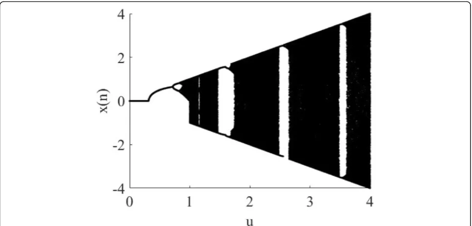
Feigenbaum equation is a one-dimensional chaotic equation [21] and is defined below:

xnþ1¼μsinðπxnÞ ð7Þ

where −4≤xn≤4, μ∈ (0,4), let the initial value x1 be

0.5; Fig.3is acquired by iterating different parameters μ for 200 times.

Whenμ< 0.315, the iterative valuexnconverges to 0; When 0.315 <μ< 0.719, the iterative value converges to a non-zero value, and the steady-state solution of sys-tem is the fixed point;

When μ≥0.719, the system becomes period doubling bifurcation, which means that two periods become four periods, and four periods become eight periods.

When μ≥0.870, the iterative value is in a state of

pseudo-random distribution, and the system becomes chaotic.

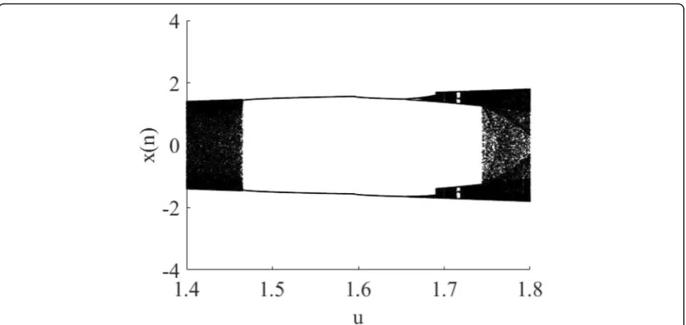
After the system became chaotic, there would be a blank area [22]; it could be found from Fig. 3 that in certain intervals of μ ∈ (1.4–1.8), the iterative value converges to certain fixed value and presents an

obvi-ous blank area. As shown in Fig. 4, when μ= 1.63, the

system converges to two fixed non-zero value and be-comes a periodic function without any chaotic features.

The blank area mapped by chaos may exist in all positions within the taking value interval of parameter

μ. When using the typical Feigenbaum equation in

the WSN positioning, different parameters μ and

ini-tial value x may be corresponding with the pathway

of blank area, and because of the lack of sample space, the randomness of sequence may be quite bad and the ergodicity of system will be seriously influ-enced [22, 23].

Because the chaotic features of logistic chaos map-ping are quite sensitive to initial value [24], the dy-namic initial value can be used to make the iteration of chaos mapping performed in different pathways to avoid the blank area. In this paper, by using the Feigen-baum equation featured by secondary coupling, the three-dimensional Feigenbaum logistic mapping based on initial value disturbance is proposed. The equation

changes the initial value ωn through logistic mapping

makes the iterative value in different chaotic pathways, so as to avoid the blank area.

The mapping of improved chaotic equation is shown in Eq. (8):

is 300. The results of the previous 100 iterations are abandoned, the iteration diagram which includes the

control parameter r and the iterative value of

se-quence x of improved Feigenbaum mapping (the

it-erative diagram of sequence y, z is similar to that in

Fig. 5), as shown in Fig. 5:

When r< 0.315, after multiple convergences, the itera-tive sequence value is equal to 0;

When r< 0.719, the iterative sequence is a non-zero fixed value;

When r> 0.753, the chaotic mapping has negative

value and becomes chaotic, and the whole chaotic space has no blank area.

Choosing proper initial value for iterative computa-tions, a sequence within the interval [−1,1] is acquired

by dividing the sequence x by r value. The results of

Eq. (6) are mapped to the interval [−1,1] by using the features of the logistic mapping function.

Lij¼

2 Faveragecij−dijmin

dijmaxþdijmin ð 9Þ

According to the three-dimensional chaotic Eq. (8)

and formula (9), new chaotic entity is acquired by add-ing the chaotic variables into searched entities. The newly acquired entity is transformed according to

for-mula (10). Where di min and di max represent the

minimum and maximum of range of anchor node, respectively.

the unknown nodes, [aj, bj] represents the minimum

and maximum of position range of unknown nodes, and it satisfies xj∈[aj, bj], the reversed solution of X is

given by: X* = (x*1, x*2…x*D). The unknown reverse

value of nodes is calculated to better shrink the posi-tioning information of space.

Formula (12) is acquired by solving reversely the

formula (11):

Comparing the node position in formula (13), the

minimum is selected as the reliable position of unknown

nodes. Xij is further positioned by using the weighted

least square estimation, and the formula (14) is acquired:

Xwls¼ ATW

−1

WB ð14Þ

where A is the weighting matrix and used to ensure

thatXwlsis agonic andWis the symmetric matrix.

3.2 Description of algorithm improvement

The algorithm improvement includes four steps which are described below:

Step 1: Collecting the average hop count and position information of anchor nodes

Step 2: The anchor node acquires the average hop distance of other anchor nodes according to formulas3

and5, calculates the stability of the anchor node and surrounding anchor nodes, and informs the other nodes in the wireless sensor network

Step 3: The unknown nodes calculate the initial position with formula6based on the average hop distance of anchor nodes in Step 2

Step 4: The precise node position is calculated by substituting the unknown node position in Step 3 into the formulas13and14

4 Simulation experiment

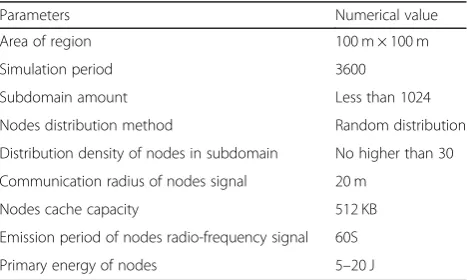
Choosing proper initial valueu1= 0.2;u2= 0.3; u3= 0.5;

r= 3; k= 3.93, w1= 0.6, conducting iterative

computa-tions on chaotic equation, and adopting Matlab simula-tion experiment environment, the Colliner precision

positioning (CPP) algorithm [25], which is widely

applied in the control group, and the analysis are performed from four indexes of terminal position preci-sion, positioning error precipreci-sion, positioning time-delay, and energy consumption bandwidth. The specific

simulation parameters are shown in Table1:

4.1 Terminal position precision

Figure6 showed the comparison of the algorithms

pro-posed in this paper and by literature [25] and [27]. It can be known from the figure that with the continuous increase of network nodes, there is a little fluctuation on the terminal position precision of the algorithm in this paper, and precision is always higher, while a sharp fall appeared on that of the algorithms of literature [25] and [27]. The algorithm in this paper has higher preci-sion because it introduced the self-adapting radio fre-quency inference which is able to ensure the channel holding at a higher level when there are fluctuations on network topology; while both the algorithms of litera-ture [25] and [27] use the fixed channel distribution mode, once there are fluctuations on the network top-ology, the channel holding will be unavailable and the terminal position precision will decrease.

4.2 Positioning error precision resent the estimated unknown nodes and the actual

unknown nodes, respectively,R is the communication

radius of nodes, the results are shown in following formula [26]:

In the experiment, the algorithms proposed in this paper and by literature [25] and [27] are compared for positioning error by setting different proportion of an-chor nodes and communication radius. Each algorithm is operated for 100 times, and the results of three algo-rithms are compared based on average value.

Figure 7 showed the comparison of the positioning

error precision of three algorithms with different nodes density; it can be known from the figure that with the continuous increase of network density, the positioning error precision of the algorithm in this paper is always higher than that of the control group, and this is because the algorithm in this paper uses the resource scheduling

mode based on radio frequency inference and the WSN’s

demand of serving for resources is satisfied by fixing the service time when the node density increase continu-ously. While the algorithms proposed by literature [25] and [27] do not take the influence of density on network congestion into account, it is difficult to improve the quality assurance demand of WSN flow of service when there is a network congestion; therefore, the positioning error precision of literature [25] and [27] is much lower than that of this paper.

With two different communication radiuses, the node positioning error of the algorithm in this paper is fewer than that of two other algorithms. This indicates that the positioning precision of the algorithm in this paper is higher than two other algorithms. It can be found from the figure that the error is bigger when the propor-tion of anchor nodes is lower. The main reason is that the number of unknown nodes is much more than the anchor nodes, and the computational error occurs be-cause the distance of many unknown nodes depends on few anchor nodes. In addition, the distance between the unknown nodes and the anchor nodes is far; there are many hops, which results in some influences on the

average hop distance. And it can be found from Figs. 8

and 9 that with the increases of communication radius,

the positioning error reduces, because the chaotic optimization which optimized the influence of commu-nication radius on average hop distance to a certain ex-tent is used in positioning error.

4.3 Positioning time-delay

Figure 10 showed the comparison of the positioning

time-delay of the algorithms proposed in this paper and by literature [25] and [27]; it can be known from the figure that with the continuous increase of nodes density, the network is at high density node and low density node and the positioning time-delay index of

Table 1Simulation parameters

Parameters Numerical value

Area of region 100 m × 100 m

Simulation period 3600

Subdomain amount Less than 1024

Nodes distribution method Random distribution

Distribution density of nodes in subdomain No higher than 30

Communication radius of nodes signal 20 m

Nodes cache capacity 512 KB

Emission period of nodes radio-frequency signal 60S

the algorithm in this paper is always lower than that of the control group. The algorithm in this paper adjusts the service quality dynamically according to the current network situation; therefore, it has a lower po-sitioning time-delay index and is not proportional to the changes of nodes density distribution, while the al-gorithms of literature [25] and [27] conduct the re-source matching according to the nodes which are able to provide resources in the network, when the nodes do not match the resources, the channel holding will be interrupted; in addition, although the algorithms of literature [25] and [27] conduct the bubbling matching for nodes density distribution, making the resource

planning only in the way of resources matching by the best nodes is quite possible to result in serious conges-tion; consequently, the positioning time-delay index of the algorithm in this paper is lower than that of the control group.

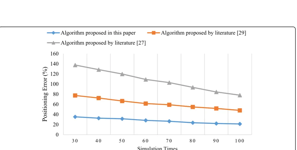
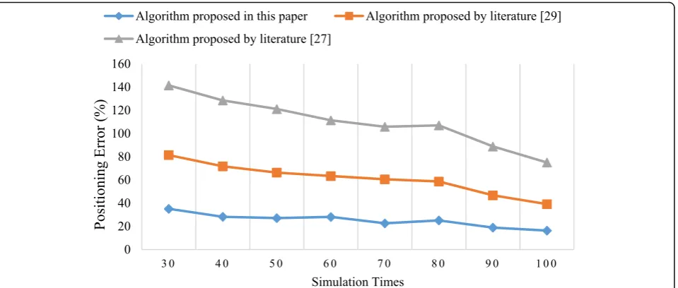
4.4 Influence of topology

Different topologies have different influences on posi-tioning error [28]; in this paper, the network topology described in literature [28] is taken as the test standard, where the network topology with general rules is the topological structure 1, the network topology of type C is the topological structure 2, and the actually simulated

Fig. 6Relationship between the terminal position precision and network nodes. Figure shows the comparison of the algorithms proposed in this paper and by literature [25] and [27]

network topology is the topological structure 3. The

al-gorithm in this paper, DV-HOP alal-gorithm [29], and the

algorithm in literature [27] are compared in the three topological structures, the results are shown in the fol-lowing figures:

It can be found from Figs. 11,12, and13 that for the error rates under the three topological structures, the algorithm in this paper is advantageous and the

posi-tioning precision has been improved. In Fig. 11, the

topological structure is good in performance, and the algorithm in this paper obviously helps improve the

successful implementation. In Fig. 12, the nodes in

topological structure are not distributed evenly, but the algorithm in this paper makes the average hop distance of each unknown node more conforming with the ac-tual situation, and improved the success rate of node positioning. Figure 13 verified the positioning error in case of nodes being close to side boundary. It can be

Fig. 8Error change when proportion of anchor node at communication radiusr= 10m. Figure shows the error change of three algorithms when proportion of anchor node at communication radiusr= 10m, each algorithm is operated for 100 times

Fig. 10Positioning time-delay test of three algorithms under different network nodes density. Figure shows the comparison of the positioning time-delay test of three algorithms under different network nodes

found that the algorithm in this paper resolved this problem effectively to a certain degree.

4.5 Comparison of convergence performance

Assuming that the distance measurement error is 20%, the algorithm in this paper, particle swarm optimization

(PSO) algorithm [26], and discrete PSO (DPSO)

algo-rithm [31] are compared for convergence performance,

and the simulation results are shown in Fig. 14. It can

be found from Fig. 14 that with the increases of

iter-ation times, at the initial moment, the fitness values of three algorithms have a sharp fall and tend to be stable after 10 iterations, which indicated that all the three

algorithms are converged. The algorithm in this paper begins to converge after 12 iterations and shows better convergence performance, while the PSO algorithm be-gins to converge after 18 iterations and the DPSO algo-rithm begins to converge after 16 iterations, which proved that the algorithm in this paper is better than the PSO algorithm.

4.6 Relationship between different iteration times and positioning error

The algorithm in this paper is compared with the ro-bust quadrilateral-based modified PSO (RQ-PSO) algo-rithm [30] and DPSO algorithm [31] in the experiment;

Fig. 12Error rates of three algorithms under topological structure 2

the relationship of their iteration times and the

posi-tioning error is shown in Fig. 15. It can be seen from

the simulated picture that the positioning error of three algorithms reduces with the increases of iteration times; among them, the slope of curve of the algorithm in this paper is the biggest, that of the RQ-PSO is smaller, and that of the DPSO is the smallest. The algorithm in this paper tends to be stable after 14 iterations and the posi-tioning error keeps being unchangeable, while the RQ-PSO algorithm keeps being stable after 18 itera-tions and the DPSO algorithm’s positioning error keeps being unchangeable after 20 iterations. This proved that the convergence speed of the algorithm in this paper is

faster than that of RQ-PSO algorithm and DPSO algo-rithm and has a proper positioning error.

5 Conclusion

The node positioning in wireless sensor network is al-ways the focus of research. In this paper, on the basis of DV-HOP algorithm, the improvement was performed from aspects of improving the error precision and least square estimation. The simulation experiment demon-strated that the effect of the algorithm proposed in this paper is obvious, and in case of continuously increasing spending in hardware, the node positioning precision in wireless sensor network had been effectively improved;

Fig. 14Comparison of algorithms convergence performance

therefore, the estimated distance between unknown nodes and anchor nodes became more precise. In net-works where little anchor nodes are necessary, the precise positioning for plenty of unknown nodes is realizable. The algorithm proposed in this paper has also a reference value for other positioning problems such as mobile communication.

Abbreviations

AOA:Angle of advent-based positioning algorithm; CPP: Colliner precision positioning algorithm; DPSO: Discrete PSO algorithm; DV-HOP: Distance Vector-HOP; PSO: Particle swarm optimization; RQ-PSO: Robust quadrilateral-based modi-fied PSO algorithm; RSSI: Received signal strength indicator-based algorithm; TDOA: Time difference of advent-based positioning algorithm; TOA: Time of advent-based positioning algorithm; WSN: Wireless sensor networks

Acknowledgements

Not applicable.

Funding

This project is supported by the Teaching Reform Project Fund of Scientific Research Fund of Guangdong Provincial Education Department under Grant (No: 416YCQ01); Teaching Reform Project Fund of Hunan province under Grant (No:2016[400]), (No:XJK17CXX002); Scientific Research Fund of Hunan Provincial Education Department under Grant (No:16C0299, 17C0295); the Natural Science Foundation of Hunan Province, China(Grant No.2018JJ2023); and Guangdong Science and Technology Plan Project under Grant 2016A020220003.

Availability of data and materials

Not applicable.

Authors’contributions

TL is in charge of the major algorithm, and numerical simulations; the others were in charge of part of the theoretical analysis and experiment. All authors read and approved the final manuscript.

Competing interests

The authors declare that they have no competing interests.

Publisher’s Note

Springer Nature remains neutral with regard to jurisdictional claims in published maps and institutional affiliations.

Author details 1

College of Mechanical Electrical Engineering, University of Electronic Science and Technology of China, Zhongshan Institute, Zhongshan, China.2_{School of} Information and Electronic Engineering, Hunan City University, Yiyang, China.

Received: 20 December 2018 Accepted: 25 April 2019

References

1. D. Gong, Y. Yang, Z. Pan, Energy-efficient clustering in lossy wireless sensor networks. J. Parallel Distrib. Comput.73(9), 1323–1336 (2013)

2. H. Dai, Q. Ye, G. Yang, et al., CSRQ: communication-efficient secure range queries in two-tiered sensor networks. Sensors16(2), 1–17 (2016) 3. X. Zhang, L. Dong, H. Peng, et al., Collusion-aware privacy-preserving range

query in tiered wireless sensor networks. Sensors14(12), 23905–23932 (2014) 4. Y. Yao, N. Xiong, J.H. Park, L. Ma, J. Liu, Privacy-preserving max/min query in

two-tiered wireless sensor networks. Comput. Math. Appl65(9), 1318–1325 (2012) 5. K. Wu, Y. Gao, F. Li, Y. Xiao, Lightweight deployment-aware scheduling for

wireless sensor networks. Mobile Netw.10(6), 837–852 (2005)

6. E. Aguirre et al., Design and implementation of context aware applications with wireless sensor network support in urban train transportation environments. IEEE Sensors J.17(1), 169–178 (2017)

7. Y. Yoon, Y.H. Kim, An efficient genetic algorithm for maximum coverage deployment inwireless sensor networks. IEEE Trans. Cybern.43(5), 1473_– 1483 (2013)

8. F.M. Al-Turjman, H.S. Hassanein, M.A. Ibnkahla, Efficient deployment of wireless sensor networks targeting environment monitoring applications. Comput. Commun.36(2), 135–148 (2013)

9. J.-H. Chang et al., An efficient relay sensor placing algorithm for connectivity in wireless sensor networks. J. Inf. Sci. Eng.27(1), 381–392 (2011)

10. L. Junfeng, P. Xiaogang, T. Lirui, Z. Yongchang,Using positioning priorities for accurate anchor-based node location over wireless sensor networks, Proceedings - 2017 IEEE 23rd international conference on parallel and distributed systems, ICPADS (2017), pp. 791–795

11. Z. Baoli, Y. Fengqi, inProc. of IEEE International Conference on Informationand Automation. An energy efficient localization algorithmfor wireless sensor networks using a mobile anchor node (IEEE Press, Zhangjiajie, 2008) 12. S. Quanyi, Z. Jinfang, Z. Jie, Wireless sensor network node localization

algorithm based on hopcount-angle factor. Comput. Eng. Des38(4), 909_– 915 (2017) (in Chinese)

13. Z. Ziwei, Z. Chao, A WS/N node localization algorithm combining centroid and DV-HOP algorithms. Comput. Appl. Soft.32(11), 130–133 (2015) 14. N.B. Priyantha, H. Balakrishnan, E.D. Demaine, et al.,Mobile Assisted

Localization in Wireless Sensor Networks[C]//Proc. OfIEEE INFOCOM’05(IEEE Press, Miami, 2005)

15. Z. Yan, Study of wireless sensor network localization algorithm based on RSSI. Comput. Sci.36(4), 119_–120 (2009)

16. B. Peng, L. Li, An improved localization algorithm based on genetic algorithm in wireless sensor networks. Cogn. Neurodyn.9(2), 249–256 (2015)

17. Z. Fengmei, Z. Li, Research on improved passive target location algorithm in WSN. Appl. Res. Comput.33(4), 1212_–1215 (2016) in Chinese

18. J. Changjiang, T. Xianlun, X. Min, Unequal clustering routing protocol for wireless sensor networks based on PSO algorithm. Appl. Res. Comput.29(8), 3074–3078 (2012) in Chinese

19. G. Zhongwen, G. Ying, H. Feng, et al., Perpendicular intersection: locating wireless sensors with mobile beacon. IEEE Trans. Veh. Technol.59(7), 3501– 3509 (2010)

20. F. Ruijuan, W. Qian, L. Qiang, Improved DV-HOP algorithm to WSN node localization on transmission line. Comput. Simul.30(9), 131_–134 (2013) in Chinese 21. L. Tu, Y. Zhang, X. Huang, L. Jia, A novel biological image encryption

algorithm based on two-dimensional Feigenbaum chaotic map. J. Chem. Pharm Res6(7), 2073–2082 (2014)

22. M. Yongyi, W. Yao, Encryption algorithm based on double chaos system with mutual feedback. J. Comput. Appl.32(10), 2768–2770,2775 (2012) (in Chinese) 23. T. Li, Z. Chi, Z. Yingzheng, J. Liyuan, A novel image encryption algorithm based

on two-dimensional general logistic mapping and output-feedback. J. Cent. South Univ. (Science and Technology)45(6), 1893_–1899 (2014) in Chinese 24. T.J.O. Kejian, Controlling the period-doubling bifurcation of logistic model.

ActaPhysica Sinica55(9), 4337–4441 (2006) in Chinese

25. B. Tang, X.R. Dong, High sensitivity GPS software receiver algorithm based on simple differential coherent accumulation. Signal Process.25(5), 832_–836 (2014) 26. Y. Peiru, X.S. Liang, Study on WSN node localization technology for

environment monitoring. Comput. Sci..45(3), 94–99,125 (2018)

27. R. Shahryar, Oppsiton-based differential evolution. Evol. Comput.12(1), 64– 79 (2008)

28. G. Yang, J. Nightingale, Special Issue on Mobile Multimedia Big Data Embedded Systems, J. Adv. Comput. Intell. Intell. Inform.22(7), 1071(2018) 29. Y. Lei, Y. Chengbo, Z. Songjian, T. Jun, L. Ru, WSN localization algorithm

based on hop distance correction weighted DV-HOP. Piezoeledtrics& Acoustooptics.35(6), 899–906 (2013) in Chinese

30. C. Lujie, L. Mingyong, Z. Lichuan, S. Yongzhao, H. Shuai, A localization method for underwater wireless sensor network based on modified particle swarm optimization algorithms. J. Northwest. Polytech. Univ.35(4), 648_–654 (2017) in Chinese