Enhanced multi task compressive sensing using Laplace priors and MDL based task classification

R E S E A R C H

Open Access

Enhanced multi-task compressive sensing

using Laplace priors and MDL-based task

classification

Ying-Gui Wang

, Le Yang

, Liang Tang

, Zheng Liu

and Wen-Li Jiang

Abstract

In multi-task compressive sensing (MCS), the original signals of multiple compressive sensing (CS) tasks are assumed to be correlated. This is explored to recover signals in a joint manner to improve signal reconstruction performance. In this paper, we first develop an improved version of MCS that imposes sparseness over the original signals using Laplace priors. The newly proposed technique, termed as the Laplace prior-based MCS (LMCS), adopts a hierarchical prior model, and the MCS is shown analytically to be a special case of LMCS. This paper next considers the scenario where the CS tasks belong to different groups. In this case, the original signals from different task groups are not well correlated, which would degrade the signal recovery performance of both MCS and LMCS. We propose the use of the minimum description length (MDL) principle to enhance the MCS and LMCS techniques. New algorithms, referred to as MDL-MCS and MDL-LMCS, are developed. They first classify tasks into different groups and then reconstruct signals from each cluster jointly. Simulations demonstrate that the proposed algorithms have better performance over several state-of-art benchmark techniques.

Keywords: Multi-task; Compressive sensing; Laplace priors; Minimum description length; Task classification

1 Introduction

If a signal is compressible in the sense that its representa-tion in a certain linear canonical basis is sparse, it can then be recovered from measurements obtained at a rate much lower than the Nyquist frequency using the technique of compressive sensing (CS) [1-3]. Mathematically, in CS, the signal is measured via

y=0θ+n=θ+n (1)

whereθ is theN ×1 original signal vector, ₀ denotes theM×N measurement matrix, denotes theN ×N linear basis,=₀,yis theM×1 compressive mea-surement vector, andnis the additive noise. SinceMis far smaller thanN, the original signal is now compressively represented, but the inverse problem, namely recovering

θfromy, is in general ill-posed. Ifθis sparse (i.e., most of

*Correspondence: [email protected]

1College of Electronic Science and Engineering, National University of Defense Technology, Deya Road, Changsha 410073, People’s Republic of China Full list of author information is available at the end of the article

its elements are zero), the signal reconstruction problem could become feasible. An approximation to the original signal in this case can be obtained through the technique of basis pursuit that solves

θ =arg min

θ θ1, s.t.

y−θ₂≤ε (2)

where ·₂ and ·₁ denote the l2-norm and the l1

-norm, respectively, and the scalarε is a small constant. Equation 2 has been the starting point for the develop-ment of many signal recovery methods in the literature. Among them, the recovery algorithms under the Bayesian framework provide some advantages over other formula-tions. These include providing probabilistic predictions, automatic estimation of model parameters, and the eval-uation of the uncertainty of reconstruction. The existing Bayesian approaches include the Bayesian compressive sensing (BCS) [4] that stems from the relevance vector machine [5] and the Laplace prior-based BCS [6].

In [7], multi-task compressive sensing (MCS) was intro-duced within the Bayesian framework. In this work, a CS task refers to the union of an original signal vector,

the measurement matrix, and the associated compressive measurement vector obtained using Equation 1. In con-trast to the CS aim of recovering a single signal from its compressive measurements, MCS exploits the statistical correlation among the original signals of multiple CS tasks and recovers them jointly to improve the signal recon-struction performance. It has been shown in [7] that MCS allows recovering in a robust manner the signals whose compressive measurements are insufficient when they are reconstructed separately. The MCS technique has been investigated extensively in machine learning literature, where it was referred to as simultaneous sparse approx-imation (SSA) [8-12] as well as distributed compressed sensing [13]. In [14], an empirical Bayesian strategy for SSA was developed.

The contribution of this paper is twofold. We shall first extend the work of [6] on the Laplace prior-based BCS to the MCS scenario. A new MCS algorithm for signal recov-ery, termed as the Laplace prior-based MCS (LMCS), is developed. We impose Laplace priors on the original sig-nals in a hierarchical manner and show that the MCS is indeed a special case of LMCS. The incorporation of Laplace priors enforces signal sparsity to a higher extent [15] and offers posterior distributions rather than point estimates as in MCS. Another advantage comes from the log-concavity of the Laplace distribution, which leads to unimodal posterior distribution and eliminates the pres-ence of local minima as a result.

The second part of this work comes from the following observation. Specifically, in order to provide satisfactory signal reconstruction performance, the MCS technique from [7], together with the newly proposed LMCS method, requires that the original signals of the multiple CS tasks are well correlated statistically. This assumption may not be fulfilled in many practical applications. For instance, some original signals may be realizations of dif-ferent signal templates that differ in their supports. In other words, they could belong to different signal groups, and the statistical correlation among them is weak, which would degrade the signal recovery performance. A possi-ble approach to address this propossi-blem is to group the CS tasks before the signal reconstruction stage, as in the MCS with Dirichlet process priors (DP-MCS) [16].

The second contribution of this paper is the use of the minimum description length (MDL) principle to augment the MCS and LMCS methods. The obtained techniques are referred to as the MDL-MCS and MDL-LMCS algo-rithms. The MDL principle has been adopted to solve the model selection problem [17-19] and can also be used in other aspects, such as sparse coding and dictionary learn-ing [20] and radar emitter classification [21-23]. In MDL, the best model for a given datay is the solution to the minimization problem ω = arg min

ω∈DL

y,ω. Here,

represents the set of possible models and DLy,ωis a codelength assignment function which defines the theo-retical codelength required to describeyuniquely, which is the key component in any MDL-based classification technique. Common practice in MDL uses the ideal Shan-non codelength assignment [24] to define DLy,ω in terms of a probability assignmentpy,ωasDLy,ω =

−log₂py,ω. Applying py,ω = py|ωp(ω), we have ω = arg min

ω∈−log2p

y|ω − log₂p(ω), where

−log₂p(ω)represents the model complexity. Note that the MCS and the new LMCS methods are both under the Bayesian framework, which enables their integration with the statistical MDL technique. Compared with the DP-MCS technique that utilizes variational Bayes (VB) inference and could suffer from local convergence, the newly proposed MDL-MCS and MDL-LMCS methods offer improved correct signal classification rate and better signal reconstruction performance. This is also illustrated via computer simulations in Section 5.

The remainder of this paper is structured as follows. In Section 2, we review the prior sharing concept in MCS and present the prior sharing framework in LMCS. Section 3 develops the proposed LMCS algorithm. We describe in Section 4 the MDL-based MCS and LMCS techniques, namely, the MDL-MCS and MDL-LMCS algorithms. Sim-ulations are given in Section 5 to illustrate the perfor-mance of the proposed algorithms. Section 6 concludes the paper.

2 Prior sharing in MCS and LMCS

In the area of machine learning, information sharing among tasks is a well-known technique [25]. Typical approaches, to name a few, include sharing hidden nodes in neural networks [26,27], assigning a common prior in hierarchical Bayesian models [28-30], placing a common structure on the predictor space [31], and the structured regularization in kernel methods [32]. Among them, the use of hierarchical Bayesian models with shared priors is one of the most important methods for multi-task learn-ing [33-37], which is also essential for the development of MCS in [7] and the LMCS algorithm in this paper. For the sake of clarity, in the rest of this section, we shall first review the prior sharing in the MCS algorithm and then proceed to present the hierarchical Bayesian framework of LMCS.

To facilitate the presentation, suppose there are LCS tasks

y_i=_iθ_i+ni (3)

i,1,. . .,i,N

. Here, θi =

θi,1,. . .,θi,N T

is the orig-inal signal for task i and the measurement noise ni is assumed to follow an i.i.d. Gaussian distribution with zero mean vector and covariance matrixβ−1I. The conditional likelihood function ofy_iis

py_i|θ_i,β=Ny_i|_iθ_i,β−1I (4)

where Ny_i|iθi,β−1Irepresents a Gaussian distribu-tion with mean vectoriθi and covariance matrixβ−1I. The noise precisionβfollows a Gamma distribution

p(β|a,b)=Ga(β|a,b)= b

a

(a)β

a−1_{exp(−bβ) (5)}

whereaandbare the shape and scale parameters of the Gamma distribution and (a)is the Gamma function.

2.1 Prior sharing in MCS

In MCS [7], the elements in θi are statistically inde-pendent, and they follow a joint Gaussian distribution:

p(θi|α)= N

j=1

N θi,j|0,α−_j 1

. (6)

Here, α = [α1,α2,. . .,αN]T is the information vector shared by the original signals θi of all the L tasks. Its distribution function is given by

p(α|c,d)=

N

j=1

Gaαj|c,d. (7)

In [7], the general strategy of setting the hyper-parameters a,c to ones and b,d to zeros in Equations 5 and 7 was adopted so that the prior ofαandβ are both uniformly distributed. As a result, they can be found via maximizing the following likelihood function:

L

i=1

py_i|α,β=

L

i=1

py_i|θ_i,βp(θ_i|α)dθ_i. (8)

This is equivalent to maximizing the posterior distribu-tion ofα andβ. The original signalsθ_i are then recon-structed using the estimated values ofαandβ.

2.2 Prior sharing in LMCS

Within the LMCS framework, the original signals are assigned Laplace priors. A possible approach to achieve this is to impose Laplace priors directly on the original sig-nal, or mathematically, letp(θ_i|λ)= λ₂exp−λ₂θ_i1as

in [6]. However, this formulation is not conjugate to the conditional distribution in Equation 4, which would ren-der the Bayesian analysis intractable. Therefore, we adopt the hierarchical prior given by

p(θ_i|γ)=

N

j=1

Nθ_i,j|0,γ_j (9)

pγ_j|λ=Gaγ_j|1,λ/2

= λ

2exp

−λγj

2

,γj≥0,λ≥0

(10)

p(λ|ν)=Ga(λ|ν/2,ν/2) (11)

whereγ =[γ₁,. . .,γ_N]T,pγ_j|λ, andp(λ|ν)are the prior distributions ofγ_jandλ, respectively. Compared with the MCS model given in Equation 6, Equation 7 reveals that in LMCS, information sharing is realized via the vector

γ and the hyper-parameterλ. We have from Equations 9 to 11

p(θi|λ)=

p(θi|γ)p(γ|λ)dγ

=

N

j=1

pθi,j|γj

pγj|λ

dγj

= λN/2

2N exp ⎛ ⎝₋√λ

N

j=1 |θi,j|

⎞ ⎠.

(12)

This verifies that the used hierarchical prior model results in Laplace priors for the original signalsθ_i.

As in MCS, LMCS recovers the original signals in a two-step manner. In particular, it first estimatesγ,λ,β, andν

via maximizing the posterior distribution

L

i=1

pθi,γ,λ,β,ν|yi

=

L

i=1

pθi|γ,λ,β,yi

pγ,λ,β,ν|y_i.

(13)

Taking the logarithm on both sides of the above equation yields

L

i=1

lnpθ_i,γ,λ,β,ν|y_i

=

L

i=1

lnpθ_i|γ,λ,β,y_i+

L

i=1

lnpγ,λ,β,ν|y_i.

It is straightforward to verify that pθi|γ,λ,β,yi

=

p(y_i|θi,β)p(θi|γ)p(γ|λ)

p(yi|θi,β)p(θi|γ)p(γ|λ)dθi =

p(y_i|θi,β)p(θi|γ)

p(yi|θi,β)p(θi|γ)dθi.

Further-more, from Equations 4 and 9, we have that it also has a Gaussian distributionNθ_i|μ_i,_iwith the mean vector and covariance matrix equal to

μ_i=β_iT_i y_i (15)

_i=βT_ii+₀−1 (16)

where0=diag(1/γ1,. . ., 1/γN).

With the estimatedγ,λ, andν, LMCS then proceeds to reconstruct the original signals from all theLCS tasks.

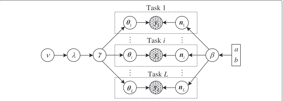
We illustrate the hierarchical prior model adopted in LMCS in Figure 1. It can be observed that, as in MCS, the distribution of the measurement noiseniis dependent on the noise precisionβwhile the prior distribution func-tions of the original signalsθ_idepend on the information sharing vectorγ. The difference here is that LMCS has one more layer of prior information, which is embedded inλ. The introduction ofλmakes the prior distribution of the original signal Laplace, which is already shown in Equation 12. As a result, the proposed LMCS would pro-mote the sparsity of the recovered signal, as pointed out in [15].

3 Multi-task compressive sensing using Laplace

priors

We shall present the proposed LMCS algorithm in this section. The LMCS method differs from the MCS tech-nique only in the step of identifying the information shar-ing vectorγ and the parametersλandνwhile their signal recovery steps are the same. As a result, we shall focus on the estimation ofγ, λ, andν. Interested readers are directed to [7] for details on the signal recovery process.

As shown in previous works [7,38,39], the signal recon-struction performance would be degraded if the noise precision β is not properly initialized. Therefore, in this work, we considerβas a nuisance parameter and integrate it out to reduce the number of unknowns and improve the robustness of the algorithm. For this purpose, the prior distributions of the original signals θ_i are rewritten as in [7]:

p(θi|γ,β)= N

j=1

Nθi,j|0,γjβ−1 (17)

whereβhas a Gamma prior distribution

p(β|a,b)=Ga(β|a,b). (18)

Note that in this case, pθi|γ,λ,β,yi

given above Equation 15 is still Gaussian with the mean vector and the covariance matrix given in Equation 15 and 16. After taking integration with respect toβ, we have

pθi|γ,λ,yi

= pθ_i|γ,λ,β,y_ip(β|a,b)dβ

= (a+N/2)

1+₂1_bθi−μi

T

−_i1θi−μi

−(a+N/2)

(a) (2πb)N/2(det(i))1/2

(19)

where det(·)is the determinant operator and

μ_i=_iT_i y_i (20)

i=

T_i i+0 −1

. (21)

Note thatpθi|γ,λ,yi

has the functional form of a Stu-dent’stdistribution, which is heavy tailed and as a result makes the LMCS algorithm more robust to the presence of outliers in the measurement noise iny_iif any, as pointed out in [40].

1

i

L

y

i

y

1

y

L

n

i

n

1

n

a

b

Task 1

Task

i

Task

L

Taking integration with respect to β on both sides of Equation 13, using Equation 19, and apply-ing the logarithm yields the posterior distribution

function L

information sharing vectorγ and the parameter λ. We begin with integratingθ_i out and applying the relation-shippγ,λ,ν|y_i=py_i,γ,λ,ν/py_i∝py_i,γ,λ,νto matrices0andiare defined under Equation 16 and in Equation 21, respectively.

In the rest of this section, we shall present two meth-ods for identifyingγ andλ. The first technique, described in Section 3.1 iteratively maximizesL(γ,λ,ν)to find the accurate solution. It has high computational complex-ity, which motivates the development of an alternative method with much lower complexity in Section 3.2.

3.1 Iterative solution

After some straightforward manipulations, we obtain

γ_j−1= nal element ofi. Following a similar approach,λcan be found to be

As in [6], we evaluateνby solving

lnν

The iterative algorithm starts with an initial solution guess onγ, λandν. We next update the estimates ofγi using Equation 24 first, then proceed to evaluate λand

ν using Equations 25 and 26. The above process would be repeated until convergence. The iterative algorithm is based on alternating optimization and is computationally intensive. One of the computational burdens lies in the evaluation of Equations 20 and 21 required in the eval-uation of Eqeval-uation 24, where inverting matrices of size N×Nis needed. This motivates the development of the following alternative algorithm.

3.2 Fast alternative solution

We start with decomposingBidefined under Equation 22

asBi=I+

. It can be verified via applying the matrix inversion lemma that the inverse ofBi

is equal toB−_i 1=B−_i,−1_j−γj

B−_i,−1_ji,jTi,jB−i,−1j

1+γjTi,jBi−,−1ji,j. With the above

notations, we are able to introduceL0(γ)that collects the

L0(γ)

DifferentiatingL0(γ)with respect toγjand setting the result to zero, we obtain

dL0(γ)

Dividing both sides withγ_i2, we can transform Equation 28 into

Applying the approximation si,j 1/γj, which is generally valid numerically (e.g., typically we have si,j > 20/γj [7]), simplifies the denominator of

The approximate solution ofγ_i−1from Equation 30 has the form

As shown in Appendix 1, on the basis of the fact that

where

Si,j=Ti,ji,j−Ti,jiiTi i,j (35)

Qi,j=Ti,jyi−Ti,jiiTiyi (36)

Gi=yTiyi−yTi iiTi yi+2b. (37)

We summarize the procedure of the fast algorithm in Algorithm 1. The convergence criterion there is

$$L0γk−L0γk−1$$

$$max(L₀(γ))−L₀γk$$ <thresh (38)

where L0

γk _{is the increment of L}

0(γ) in the kth

iteration and thresh denotes a pre-specified threshold value. To improve the convergence speed, in step 5 of Algorithm 1, we select the γ_jk that leads to the largest increase inL0(γ). Other steps in the algorithm,

includ-ing updatinclud-ingμ_i,_i,si,j,qi,j, andgi,jin steps 10 to 11 and changing the model as in steps 6 to 8, are the same as those detailed in 6 of [7].

Algorithm 1 FAST LMCS

1 Inputs:=[₁,. . .,_L],Y=y₁,. . .,y_L,thresh 2 Outputs:γ =[γ1,. . .,γN]T,λ

3 Initializeγj=0,j=1,. . .,N, andλ=0. Setk=0 4 whileconvergence criterion (38) not metDo

5 Select a particularγ_jkout ofγk =γ₁k,γ₂k,. . .,γ_NkT

6 ifA0<0 andγjk =0,thenaddγjto the model 7 else ifA0<0 andγ_jk >0,thenfindγ_jk+1using (32)

8 else ifA0>0,thenpruneγjand setγjk+1=0 9 end if

10 Updateμ_iandi 11 Updatesi,j,qi,jandgi,j

12 Updateλandνusing (25) and (26) 13 k=k+1

14 end while

Before the end of this section, we shall illustrate the relationship between the MCS algorithm and the newly proposed LMCS technique, in order to gain more insights. Within the MCS framework, the elementsγjin the infor-mation sharing vectorγ are found via [7]:

γ_jMCS=arg max γj

%

−1

2 L

i=1

ln1+γ_jsi,j

+(Mi+2a)×ln

1− γjq

2 i,j/gi,j 1+γ_jsi,j

& .

(39)

On the other hand, from Equation 27, we have LMCS that obtains the estimate ofγjthrough

γ_jLMCS=arg max γj

%

−1

2 L

i=1

ln1+γjsi,j

+(Mi+2a)×ln

1− γjq

2 i,j/gi,j 1+γjsi,j

+λγ_j

& .

(40)

Clearly, LMCS would reduce to MCS if λ = 0. This is somewhat expected from the comparison presented at the end of Section 2, where we show that, compared with MCS, LMCS introduces another layer of prior informa-tion embedded in the parameterλ. Whenλ = 0, we can

verify thatA0= L i=1

si,j−(Mi+2a)q2i.j/gi,j

si,j−q2i.j/gi,j

si,j

,B0=L, andC0=0.

As a result, Equations 32 and 33 would become

γ_j−1≈ L

L i=1

(Mi+2a)q2i.j/gi,j−si,j

si,j−q2i.j/gi,j

si,j

,

if L

i=1

(Mi+2a)q2_i.j/gi,j−si,j

si,j−q2i.j/gi,j

si,j

>0

(41)

γ_j−1= ∞, otherwise (42)

which are identical to the approximate solutions to Equation 39 established in [7] (see Equations 39 and 40 in [7]). This corroborates the validity of the Bayesian derivations that lead to LMCS.

4 MDL-based task classification and signal

reconstruction

section with the theoretical derivation of the MDL-based classification for MCS and LMCS.

4.1 MDL-based classification

This subsection presents the basic MDL-based task clas-sification framework. With MDL, the best model out of a family of competing statistical models for a given data is the one that yields the minimum description length for the data. LetY='y₁,. . .,y_L(be the set collecting the com-pressive measurements of theLCS tasks in consideration andι = [ι₁,. . .,ι_L] be the partition of Y intoK clusters, where ι_i = k means that y_i belongs to the kth cluster, i =1,. . .,L, andk =1,. . .,K. Assuming statistical inde-pendence among signals from two different clusters, we can express the likelihood function of Y as

p(Y|D,ι)=

dk is the model parameter vector of the model for the kth cluster,Ykcontains the compressive measurements of the CS tasks in thekth cluster, andpk(Yk|dk)represents the likelihood function ofYk. The description length ofY under the model setDis then

DL(Y,K)=DL(Y|D,ι)+DL(D,ι) (44)

where DL(Y|D,ι) = −log₂p([Y|D,ι]δ) measures the goodness of fit between the data and the model. Under the assumption that the model parameter setDand the CS task partitionιare statistically independent, we have DL(D,ι) = −log₂p([D]δ)−log2p([ι]δ), and it acts as a penalty function measuring the model complexity. The notation [·]δdenotes elementwise quantization with pre-cisionδ. With sufficient quantization precision, we have p([Y|D,ι]δ) ≈ p(Y|D,ι) δSY,p([D]δ) ≈ p(D) δSD, and

We proceed to evaluate Equation 45 for the cases of LMCS and MCS sequentially. In particular, as shown in Appendix 2, we have that for LMCS,

−log₂p Y|DLMCS,ι

contains the information sharing parameters of the kth

cluster, B(_ik) = I(k)₊(k) the kth cluster. Other variables are the same as those in Equation 22.

For MCS, according to Equation 30 in [7], we have

whereDMCS=

) dMCS_k

*

is the set of model parameters for

MCS,dMCS_k = )

α(_MCSk) *,α(_MCSk) is the information sharing

vector of clusterk,C(_ik) = I(k)+(_ik) A(_MCSk)

−1 (_ik)

T ,

andA(_MCSk) = diag α(_MCSk)

. In MCS,A(_MCSk) is distributed

uniformly, so −log₂pDMCS would be a constant (see Section 2.1).

We now compute −log₂p(ι) to complete the evalua-tion of Equaevalua-tion 45 for LMCS and MCS. Let n(L,ι) be the number of different ways to partitionLtasks intoK

groups with each group havingL_kCS tasks and K k=1

L_k =

L. It can be verified thatn(L,ι)is equal to

n(L,ι)= C

L1

L C L2

L−L1· · ·C

LK−1

L−L1−···−LK−2

(K−1)!m1!m2!. . .mL!

. (48)

The numerator represents the number of different parti-tions if we generate them by taking sequentiallyLk tasks out of theLCS tasks while the denominator removes the partitions produced by simply swapping the tasks within a cluster without changing the clustering structure. Assum-ing that the ι has the prior of a uniform distribution, we have

−log₂p([ι]δ)≈ −log2p(ι)−log2δL

= −log₂ 1

n(L,ι)−Llog2δ

=log₂n(L,ι)−Llog₂δ.

(49)

Putting Equation 4) together with Equation 46 or 47 back to Equation 45 completes the description length computation for the compressive measurement set Yof theLCS tasks under LMCS or MCS. Given a quantization precisionδ, the MDL criterion finds the optimal number of clustersKvia

K=arg min

1≤K≤LDL(Y,K). ₍₅₀₎

4.2 MDL-LMCS and MDL-MCS

Solving Equation 50 directly may be computationally prohibitive since it requires calculating the description length of Y for all possible clustering structures. To

address this difficulty, we shall propose the new MDL-LMCS and MDL-MCS algorithms for classifying the CS tasks and recovering all original signals in a joint and iterative manner. The algorithm flow is summa-rized in Algorithm 2. It takes as its input the sets Y

and that collect the compressive measurement vec-tors and the measurement matrices in the L CS tasks, respectively.

Since the tasks have not been classified at the beginning, the algorithm considers that they belong to a single cluster

clust{1} = {Y,}, and as a result, it sets K, the num-ber of obtained clusters, to be 1, andnum, the number of unclassified tasks, to beL. The algorithm also initializes Yand, the sets that collect the compressive measure-ments and the measurement matrices of the unclassified tasks, as Y=Y and =. Signal reconstruction via LMCS or MCS for MDL-LMCS or MDL-MCS is then performed usingYandto obtain the reconstructed sig-nal set 1 and the sharing parameter set D1. We plug

D1into Equation 46 or 47 to calculate the total

descrip-tion length (TDL)mdl1for all the compressive

measure-ments inY. This completes the initialization stage of the algorithm.

The proposed algorithm proceeds to classify theLtasks as follows. In the first iteration, it first applies the oper-ation CLASSIFY(·) to form a new cluster 'Ymin,min

(

from the unclassified task setY.Ymin hasLmintasks and

their measurement matrices are collected in _min. We removeYmin and min fromYand to update them,

while the number of remaining unclassified task becomes num−Lmin. Now, we haveK = 2 clusters, clust{1} = { ˆY,ˆ}, and clust{2} = { ˆYmin,ˆmin}a. LMCS or MCS

is then applied to both clusters to identify their original signals and sharing parameters. The results are kept in

2 and D2, the latter of which is substituted into (46)

or (47) for MDL-LMCS or MDL-MCS to compute again the TDL ofY, denoted by mdl2. This completes the

pro-cessing of iteration 1. We then compare mdl1with mdl2

and if mdl2 < mdl1, the algorithm would start its

sec-ond iteration to continue the task classification, where CLASSIFY(·) will be applied toYˆ and yieldclust{3}. The above process is repeated untilmdlK > mdlK−1occurs,

which implies the appearance of over-fitting. The algo-rithm finally outputs the clusters available in the(K−2)th iteration.

DL(_LMCSt) y_i

We next perform a grouping operation on the obtained num−1 description lengthDL(_LMCSt) y_ito identify those tasks in Yˆ that are likely to correlate well with y_i and should be grouped with y_i in a new cluster Yˆmin (see

Algorithm 2). Recall that each description length indeed corresponds to a task inYˆ other than y_i. The grouping procedure is based on the well-known K-mean tech-nique. The difference here is that before the application

of the K-mean, we first compute the algorithmic mean ofDL(_LMCSt) y_iand set those above the mean value to be equal to the mean. This is equivalent to excluding the tasks that lead to large value ofDL(_LMCSt) y_iwhen being paired with y_i because they are unlikely to be well correlated withy_i. We next applyK-mean to the remaining descrip-tion length to obtain two groups. The mean descripdescrip-tion length for both groups are found. The tasks belonging to the group with a smaller mean description length are com-bined withy_ito produce the output of CLASSIFY(·),Yˆmin.

In the case of MDL-MCS, CLASSIFY(·) is realized in the same manner as described above, except that the descrip-tion length fory_iis evaluated over every two-task cluster using

4.3 Implementation aspect

The development of MDL-LMCS and MDL-MCS pre-sented in the previous subsection implicitly assumes that the quantization precisionδis knowna priori. Neverthe-less, in an ideal case,δshould be determined jointly with the optimal number of clustersKthrough minimizing the right-hand side of Equation 50 with respect toδandK.

We shall follow the approach similar to the one adopted in [20] to determine the quantization precision. First, it can be verified that the value ofδwould have no impact on locating the unclassified tasks that are correlated with a randomly selected one if the compressive measure-ment vectors of all the tasks have the same dimension. This is because, in this case, the term depending onδ in Equations 51 and 52 would be the same for any value of t. As a result,δ will affect the task classification perfor-mance via Equations 46 and 47 only, from which it can be seen that a very fine quantization would lead to a smaller number of clusters. This may degrade the signal recon-struction performance as weakly correlated signals may be recovered jointly. A large value ofδwould not necessarily improve performance, as in this case, the original signals may tend to be recovered separately. Our experiments suggest thatδbe within the range of 0.01 to 0.1, depend-ing on the type of data to be processed. Throughout the experiments in Section 5, we shall fixδto be 0.1, instead of attempting to optimize it for different experiments.

5 Simulations

Monte Carlo (MC) simulations using synthetic data and images are performed to illustrate the performance of the LMCS algorithm developed in Section 3 and the MDL-augmented MCS algorithms, namely, the MDL-LMCS and MDL-MCS techniques presented in Section 4.

5.1 Synthetic signals

In each simulation of this subsection, the length of the original signals of all the CS tasks is fixed at N = 512, and we generate two sets of results. One set of results is produced when the non-zero elements of the original sig-nals take binary values±1 in a random manner. The other set is generated with the non-zero elements of the original signals being independently drawn from zero-mean Gaus-sian distribution with unit variance. The elements of the measurement matrix of any CS task, on the other hand, can only be drawn from a Gaussian distribution with zero mean and variance one. Each column of any measurement matrix is normalized to have a unit norm.

For the purpose of comparison, we implement the BCS and MCS techniques developed in [4] and [7]. We shall denote them as ST-BCS and MCS in the figures. Here, ST stands for single task, and it is introduced to highlight that ST-BCS and MCS recover the original signals separately and jointly. We also implement the Laplace prior-based

BCS proposed in [6] and denote it as LST-BCS. When implementing the three benchmark algorithms (ST-BCS, MCS, and LST-BCS) and the three proposed methods (LMCS, MDL-LMCS, and MDL-MCS), we always initial-izea=103_{andb=1 so that the noise precisionβhas the}

same prior distribution for all the algorithms considered (see Equation 5).

We shall follow the previous works [4,6,7] that proposed the three benchmark methods and use the average nor-malized signal reconstruction error as the primary per-formance metric. It is defined as1_LL_i=1θ_i−θˆ_i

2/θi2,

where θ_i andθˆ_i are the true and the estimated original signal vectors of the ith CS task. Note that the aver-age normalized signal reconstruction error measures the Euclidean distance between the waveforms of the recov-ered and the original signals. It is not very informative regarding the quality of the recovered signal supports. Therefore, we shall also include in some experiments per-formance results of different algorithms in recovering the signal supports, which are quantified by the average incor-rect support recovery ratio 1_LL_i=1||S(θ_i)−S(θˆ_i)||0/N.

Here, || · ||0 denotes the l0-norm and S(x) sets all the

non-zero elements inxto be 1.

5.1.1 LMCS

We consider the case ofL=2 CS tasks as in [7], in order to illustrate the performance of the proposed LMCS tech-nique and the existing methods under a simulation setup already used in the literature. The original signal of each task contains 64 non-zero elements at random locations. Zero-mean Gaussian noise with a standard deviation of 0.01 is added to the two obtained compressive measure-ment vectorsb.

In the first simulation, we illustrate in Figure 2 the impact of different choices of the parametersλandνon the performance of LMCS. The two signals are assumed to have 75% of their non-zero elements overlapped. We realize LMCS withλ= 0,λ=1,λ= 2, andλestimated using Equation 25. The results shown are averaged over 200 runs. In particular, Figure 2a,b plots the average sig-nal reconstruction error as a function of the number of compressive measurements for the two cases where the original signals are random binary numbers±1 and zero-mean Gaussian random variables with unit variance. The results show that in both cases, the reconstruction error of LMCS gradually improves as the number of compres-sive measurements increases, and the best performance is obtained whenλ is estimated using Equation 25. More-over, we can see that the LMCS with ν = 0 and ν

165 170 175 180 185 190 195 200 0

0.1 0.2 0.3 0.4 0.5 0.6 0.7 0.8 0.9 1

Number of Compressive Measurements

Average Reconstruction Error

LMCSλ =0 (MCS) LMCSλ=1 LMCSλ=2 LMCSλ est ν=0 LMCSλ est ν est

(a)

125 130 135 140 145 150 155 160 0

0.1 0.2 0.3 0.4 0.5 0.6 0.7 0.8

Number of Compressive Measurements

Average Reconstruction Error

LMCSλ =0 (MCS) LMCSλ=1 LMCSλ=2 LMCSλ est ν=0 LMCSλ est ν est

(b)

Figure 2Performance comparison of LMCS with different choices ofλandν.(a)Binary original signals and(b)Gaussian original signals.

as follows. The value ofν, when it is identified together with λ, is generally non-zero but less than one in this simulation. Careful examination of Equation 25 that gives the estimate ofλreveals that the impact of a small non-zeroνonλis negligible, when the original signal length N is large (in this section,N = 512) and the measure-ment noise level is low, which implies a large value of the noise precision β, and as a result, large values of the hyper-parametersγjfor original signals having a unit variance (see Equation 17). Therefore, in the remaining simulations, we fix ν at zero when realizing LMCS and MDL-LMCS.

It is worthwhile to point out that rigorously, ν = 0 is a boundary value for the Gamma distribution. As ν

approaches 0, the prior distribution of λ would pro-vide vague information on λ as p(λ) ∝ 1/λ (also see Equation 19 in [6]). However, this would not change the fact that Laplace prior is imposed on the original signals, as shown in Equation 12. In other words, LMCS would still outperform MCS because it enhances the sparsity con-straints on the non-zero elements of the original signals.

This is also supported by the following simulation results (see Figures 3 and 4).

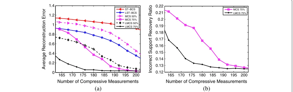
Figure 3 demonstrates the impact of the correlation between the two original signals on the performance of LMCS. It considers the cases when the two original signals have binary non-zero elements, and they have 75% and 50% of their non-zero elements overlapped. Figure 3a,b plots the average signal reconstruction error and the incorrect support recovery ratio of LMCS as a function of the number of compressive measurements. The results shown are averaged over 50 runs. For comparison, we also include in the figures the results from ST-BCS, LST-BCS, and MCS. We can observe from Figure 3a that LMCS and MCS outperform greatly over ST-BCS and LST-BCS due to the utilization of the prior sharing mechanism (see Section 2). The performance of LMCS and MCS improves as the number of the overlapping non-zero elements in the two original signals increases, as expected. More impor-tantly, LMCS exhibits superior performance in terms of a much lower signal reconstruction error over MCS for the two cases where the two original signals have 75% and 50%

165 170 175 180 185 190 195 200 0

0.2 0.4 0.6 0.8 1 1.2 1.4

Number of Compressive Measurements

Average Reconstruction Error

ST−BCS LST−BCS MCS 50% MCS 75% LMCS 50% LMCS 75%

(a)

165 170 175 180 185 190 195 200 0.12

0.13 0.14 0.15 0.16 0.17 0.18 0.19 0.2 0.21 0.22

Number of Compressive Measurements

Incorrect Support Recovery Ratio

MCS 75% LMCS 75%

(b)

125 130 135 140 145 150 155 160 0

0.1 0.2 0.3 0.4 0.5 0.6 0.7 0.8 0.9

Number of Compressive Measurements

Average Reconstruction Error

ST−BCS LST−BCS MCS 50% MCS 75% LMCS 50% LMCS 75%

(a)

125 130 135 140 145 150 155 160 0.12

0.13 0.14 0.15 0.16 0.17 0.18 0.19 0.2 0.21 0.22

Number of Compressive Measurements

Incorrect Support Recovery Ratio

MCS 75% LMCS 75%

(b)

Figure 4Comparison of ST-BCS, LST-BCS, MCS, and LMCS in reconstructing signals with Gaussian non-zero elements.(a)Average reconstruction error and(b)incorrect support recovery ratio.

of their non-zeros overlapped. The performance enhance-ment mainly comes from the use of Laplace priors on the original signals in LMCS. Compared with MCS, LMCS imposes another layer of prior information on the hyper-parameters of the original signals, which makes MCS a special case of LMCS as shown in Equations 39 and 40 at the end of Section 4. As a result, LMCS offers more flexi-bility in modeling the sparsity of the original signals. This is also corroborated by Figure 3b, where it shows that in the case where the two original signals have 75% of their non-zero elements colocated, LMCS can provide a lower incorrect support recovery ratio and can better recover the sparse signal support.

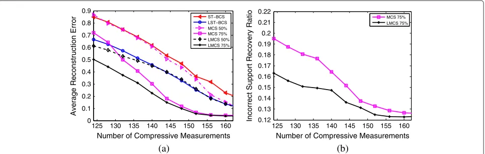
Figure 4 repeats the simulation experiment in Figure 3, but it considers the case where the two original sig-nals have the non-zero elements drawn from zero-mean Gaussian distribution with unit variance. The obtained observations are similar to those in Figure 3.

5.1.2 MDL-based task classification and signal reconstruction

In this subsection, we present simulation results to illus-trate the performance of MDL-MCS and MDL-LMCS developed in Section 4. For the purpose of comparison, we also show the results of the ST-BCS, LST-BCS, MCS, and LMCS methods as well as the DP-MCS technique.

The simulated algorithms are used to recover the origi-nal sigorigi-nals ofL=40 CS tasks that belong to eight clusters with five tasks each. Every cluster has its own signal tem-plate that differs in the signal supports. All the original signals have 64 non-zero components, and their locations are initially chosen so that the correlation between any two original signals from different clusters is zero. Later, we perform the following perturbation to induce slight correlation among clusters. Specifically, in each ensem-ble run, six non-zero elements in each signal template are selected randomly and set to zero elements, while at

the same time, six elements that are zeros in the original template are reset to be non-zeros. In this way, the five sig-nals within the same cluster are highly correlated, but the signals from different clusters have distinct sparsity struc-tures. The simulation results are obtained via averaging over 50 ensemble runs.

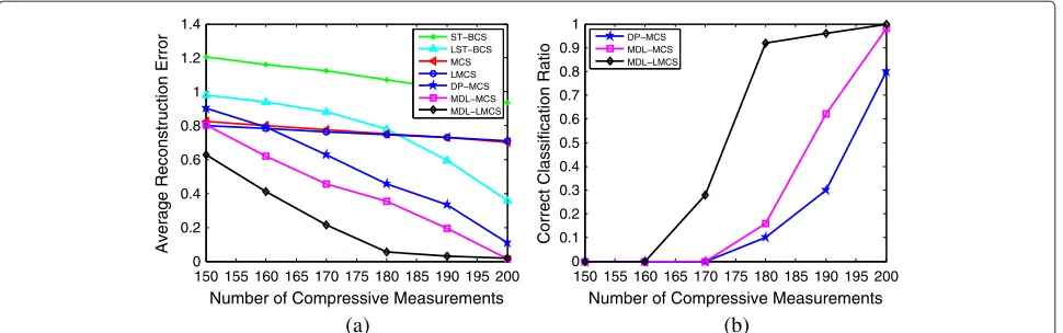
In Figure 5a,b, we plot as a function of the number of compressive measurements the binary signal recon-struction error and the correct task classification ratio of the simulated seven algorithms. As we can see from Figure 5a, pretending that the 40 CS tasks belong to the same group and recovering the original signals using LMCS or MCS would lead to a signal reconstruction error even higher than reconstructing the original sig-nals separately via LST-BCS. This clearly demonstrates the impact of incorrect task classification on the signal recovery performance. On the other hand, the proposed MDL-LMCS and MDL-MCS algorithms outperform the DP-MCS technique in terms of lower signal reconstruc-tion error. The performance improvement can be better explained by examining Figure 5b. We can see that the application of the MDL principle to augment LMCS and MCS leads to a greatly improved correct task classification ratio, compared with the DP-MCS technique. With the CS task correctly grouped, MDL-LMCS and MDL-MCS can better recover the original signals of every group.

We repeat the simulation used to generate Figure 5 with the original signals being zero-mean Gaussian random variables with unit variance. The obtained results are sum-marized in Figure 6. The observations obtained are similar to those in Figure 5.

5.2 Images

150 155 160 165 170 175 180 185 190 195 200 0

0.2 0.4 0.6 0.8 1 1.2 1.4

Number of Compressive Measurements

Average Reconstruction Error

ST−BCS LST−BCS MCS LMCS DP−MCS MDL−MCS MDL−LMCS

(a)

150 155 160 165 170 175 180 185 190 195 200 0

0.1 0.2 0.3 0.4 0.5 0.6 0.7 0.8 0.9 1

Number of Compressive Measurements

Correct Classification Ratio

DP−MCS MDL−MCS MDL−LMCS

(b)

Figure 5Comparison of signal reconstruction and classification performance for binary signals.(a)Binary signal reconstruction error and(b) correct classification ratio.

algorithms in consideration are drawn from a uniform spherical distribution.

Figure 7 summarizes the reconstruction results from a particular run. The first three images in Figure 7a, labeled as tasks 1 to 3, are taken from [7], and they belong to the same cluster. The remaining six images in Figure 7a forms another two clusters, where one cluster consists of tasks 4 to 6 and the other is composed of tasks 7 to 9. These six images are modified from the first three images via permuting randomly the intensities of the rectangles and shifting their positions by distance randomly sampled from a uniform distribution.

All original images have the dimension of 1,024×1,024. Here, we utilize the Haar wavelet expansion with a coars-est scale of 3 and a fincoars-est scale of 6. Figure 7a gives the result of the inverse wavelet transform with 4,096 samples, denoted as linear in the figure. This is the best perfor-mance achievable by all the CS algorithms considered here. The reconstruction result from DP-MCS is shown

in Figure 7b, where we adopted the hybrid CS scheme that compresses the fine-scale coefficients only as in [7] intoMi=680(i=1,. . ., 9)measurements for each task. Figure 7c,d gives the recovery results of MDL-MCS and MDL-LMCS, respectively.

We fix the original images and repeat the above exper-iment 20 times, each time with independently generated measurement matrices for all the three algorithms. In every run, the image reconstruction error for each task is evaluated and averaged to obtain the normalized image reconstruction error, which is again averaged over 20 runs to yield the average image reconstruction error summa-rized in Table 1. We also include in Table 1 the correct classification ratio.

The results in Figure 7 and Table 1 show that MDL-LMCS has the best image reconstruction and classi-fication performance, while MDL-MCS yields a better performance than DP-MCS. This is consistent with the observations obtained from Figures 5 and 6.

110 115 120 125 130 135 140 145 150 155 160 0

0.1 0.2 0.3 0.4 0.5 0.6 0.7 0.8 0.9 1

Number of Compressive Measurements

Average Reconstruction Error

ST−BCS LST−BCS MCS LMCS DP−MCS MDL−MCS MDL−LMCS

(a)

110 115 120 125 130 135 140 145 150 155 160 0

0.1 0.2 0.3 0.4 0.5 0.6 0.7 0.8 0.9 1

Number of Compressive Measurements

Correct Classification Ratio

DP−MCS MDL−MCS MDL−LMCS

(b)

Task 1

Task 2

Task 3

Task 4

Task 5

Task 6

Task 7

Task 8

Task 9

(a) (b) (c) (d)

Figure 7Comparison of DP-MCS, MDL-MCS, and MDL-LMCS in image reconstruction.(a)Linear,(b)DP-MCS,(c)MDL-MCS, and(d) MDL-LMCS.

6 Conclusions

In this paper, we first extended previous works on the Laplace prior-based Bayesian CS to the scenario of mul-tiple CS tasks and developed the LMCS technique. The hierarchical prior model was adopted to impose the Laplace priors, and it was shown that the MCS algorithm is indeed a special case of LMCS. Next, this paper con-sidered the scenario where the multiple CS tasks are from different groups, under which the performance of both MCS and LMCS would be degraded, since they attempt to recover the uncorrelated signals jointly. We proposed the MDL-based MCS techniques, namely, MDL-MCS

Table 1 Image reconstruction and classification performance of DP-MCS, MDL-MCS, and MDL-LMCS

Average reconstruction Correct classification

error ratio

Linear 0.22623

-DP-MCS 0.27647 0.35

MDL-MCS 0.24511 0.60

MDL-LMCS 0.22642 1.00

and MDL-LMCS, which first classify tasks into different groups using the MDL principle and then reconstruct sig-nals of every cluster. Simulations verified the enhanced performance of MDL-MCS and MDL-LMCS in terms of lower signal reconstruction error over the benchmark MCS and DP-MCS techniques as well as single-task CS algorithms.

Endnotes

a _{It can be easily verified that in our algorithm,Kis}

equal to the iteration index plus one. Besides,clust{1} always contains all the unclassified tasks andclust{K}is the newest cluster formed in the current iteration.

b _{Our choice of the noise standard deviation of 0.01 is}

on the same order of the values adopted in the literature. For example, in [6] and [7], the noise standard deviation is set to be 0.03 and 0.005.

Appendix 1

Derivation and analysis of Equations 32 and 33

In this appendix, we shall present the derivation that leads to Equations 32 and 33 and show that it is only a suboptimal solution to the maximization of Equation 27.

Our derivation applies the approximation that si,j 1/γj, which has been found to be valid numerically [7]. This results in the estimate of γj having the functional form given in Equation 30. When A0 > 0, both

solu-tions in Equation 30 would be negative, which violates the requirement thatγjmust be positive. IfA0 < 0, only the

solutionγ_j−1=−B0−√0

/(2A0)is valid. For the case A0= 0, from Equation 27,γjwill have the accurate solu-tionγ_j=0. This completes the derivation of Equations 32 and 33.

We next show that the solution in Equation 32 and 33 is suboptimal. For this purpose, utilizing the approximation si,j1/γjtransforms Equation 28 into

dL0(γ)

drj =

dl0

γj

drj ≈ −

1

2 γ

−2

j A0+γj−1B0+C0

.

We can also obtain easily

Substituting Equation 32 into Equation 54 yields

d2L0(γ)

This indicates that the solution in Equation 32 is the unique maximizer of the approximated version of Equation 27. However, solving Equation 29 accurately, which is equal to finding all the candidate maximizers for Equation 27, may yield two or more positive estimates ofγ_j. Among them, one would be relatively close to the approximate solution in Equation 32. In other words, the approximate solution is within the vicinity of a stationary point of Equation 27, which may only correspond to a local maxima.

Appendix 2

Derivation of Equation 46

To avoid confusion, we use superscript(k)to denote the kth cluster in the following derivation. For mathematical tractability, besides the independence among signals from two different clusters, we also assume the independence among signals within the same cluster. As a result, we have

−log₂p Y|DLMCS,ι

where Lk is the number of tasks in the kth cluster such

that parameters of thekth cluster. Similarly, assuming statisti-cal independence amongdLMCS_k , we obtain

−log₂p DLMCS

Combining Equations 56 and 57 yields

−log₂p Y|DLMCS,ι

From Equation 22, Equation 58 can be rewritten as

−log₂p Y|DLMCS,ι

Carrying out the integration, simplifying and applying some straightforward manipulations give Equation 46.

Competing interests

The authors declare that they have no competing interests.

Acknowledgements

The authors wish to thank the editor and the anonymous reviewers for their constructive suggestions. The authors thank S. Derin Babacan, Shihao Ji, and David Dunson for sharing codes of their algorithms. This work was supported in part by Hunan Provincial Innovation Foundation for Postgraduates under Grant CX2012B019, Fund of Innovation, Graduate School of National University of Defense Technology under grant B120404, and National Natural Science Foundation of China (no. 61304264).

Author details

1_{College of Electronic Science and Engineering, National University of Defense}

Technology, Deya Road, Changsha 410073, People’s Republic of China. 2_{School of Internet of Things (IoT) Engineering, Jiangnan University, Lihu Road,}

Wuxi 214122, People’s Republic of China.3_{Key Laboratory of Universal Wireless} Communications, Ministry of Education, Beijing University of Posts and Telecommunications, Xitucheng Road, Beijing 100876, People’s Republic of China.

Received: 28 April 2013 Accepted: 1 October 2013 Published: 17 October 2013

References

1. Baraniuk R, A lecture on compressive sensing. IEEE Mag. Signal Process.

24(4), 118–121 (2007)

2. E Candés, J Romberg, T Tao, Robust uncertainty principles: exact signal reconstruction from highly incomplete frequency information. IEEE Trans. Inf. Theory.52(2), 489–509 (2006)

3. DL Donoho, Compressed sensing. IEEE Trans. Inf. Theory.52(4), 1289–1306 (2006)

4. S Ji, Y Xue, L Carin, Bayesian compressive sensing. IEEE Trans. Signal Process.56(6), 2346–2356 (2008)

5. ME Tipping, Sparse Bayesian learning and the relevance vector machine. J. Mach. Learn. Res.1, 211–244 (2001)

7. S Ji, D Dunson, L Carin, Multi-task compressive sensing. IEEE Trans. Signal Process.57(1), 92–106 (2009)

8. D Leviatan, VN Temlyakov, Simultaneous approximation by greedy algorithms, Technical report, University of South Carolina (2003) 9. SF Cotter, BD Rao, K Engan, K Kreutz-Delgado, Sparse solutions to linear

inverse problems with multiple measurement vectors. IEEE Trans. Signal Process.53(7), 2477–2488 (2005)

10. JA Tropp, AC Gilbert, MJ Strauss, Algorithms for simultaneous sparse approximation. Part I: Greedy pursuit. Signal Process.86, 572–588 (2006) 11. JA Tropp, Algorithms for simultaneous sparse approximation. Part II:

convex relaxation. Signal Process.86, 589–602 (2006)

12. D Escoda, L Granai, P Vandergheynst, On the use of a priori information for sparse signal approximations. IEEE Trans. Signal Process.54(9), 3468–3482 (2006)

13. D Baron, MF Duarte, Sarvotham S, Wakin M B, Baraniuk R G, An information-theoretic approach to distributed compressed sensing, in

Proceedings of the 43rd Allerton Conference on Communication, Control, and Computing,Monticello, IL, Sept 2005

14. DP Wipf, BD Rao, An empirical Bayesian strategy for solving the simultaneous sparse approximation problem. IEEE Trans. Signal Process.

55(7), 3704–3716 (2007)

15. MW Seeger, H Nickisch, Compressed sensing and Bayesian experimental design, inProceedings of the 25th International Conference on Machine Learning,Helsinki, July 2008

16. Y Qi, D Liu, L Carin, D Dunson, Multi-task compressive sensing with Dirichlet process priors, inProceedings of the 25th International Conference on Machine Learning,Helsinki, July 2008

17. J Rissanen, Modeling by shortest data description. Automatica.14, 465—471 (1978)

18. J Rissanen, Universal coding, prediction information, estimation. IEEE Trans. Inf. Theory.30(4), 629—636 (1984)

19. A Barron, BYu J Rissanen, The minimum description length principle in coding and modeling. IEEE Trans. Inf. Theory.44(6), 2743—2760 (998) 20. I Ramirez, G Sapiro, An MDL framework for sparse coding and dictionary

learning. IEEE Trans. Signal Process.60(6), 2913—2927 (2012) 21. J Liu, SW Gao, ZQ Luo, TN Davidson, JPY Lee, The minimum description

length criterion applied to emitter number detection and pulse classification, inProceedings of the Ninth IEEE Workshop on Statistical Signal and Array Processing,Portland, OR, Sept 1998

22. KM Wong, ZQ Luo, J Liu, JPY Lee, Gao S W, Radar emitter classification using intrapulse data. Int. J. Electron. Comm.12, 324–332 (1999) 23. J Liu, JPY Lee, L Li, Z Luo, KM Wong, Online clustering algorithms for radar

emitter classification. IEEE Trans. Pattern Anal. Mach. Intell.27(8), 1185–1196 (2005)

24. T Cover, J Thomas,Elements of Information Theory, 2nd edn (Wiley, New York, 2006)

25. R Caruana, Multi-task learning. Mach. Learn.28(1), 41–75 (1997) 26. J Baxter, Learning internal representations, inProceedings of the Eighth

Annual Conference on Computational Learning Theory,Santa Cruz, CA, July 1995

27. J Baxter, A model of inductive bias learning. J. Artif. Intell. Res.12, 149–198 (2000)

28. ND Lawrence, JC Platt, Learning to learn with the informative vector machine, inProceedings of the 21st International Conference on Machine Learning,Banff, Alberta, July 2004, 65

29. K Yu, V Tresp, Schwaighofer A, Learning Gaussian processes from multiple tasks, inProc. 22nd Int. Conf. Mach. Learn.(ICML 22), 2005

30. J Zhang, Z Ghahramani, Y Yang, Learning multiple related tasks using latent independent component analysis, inAdvances in Neural Information Processing Systems (NIPS),Vancouver, British Columbia, Dec 2006 31. RK Ando, T Zhang, A framework for learning predictive structures from

multiple tasks and unlabeled data. J. Mach. Learn. Res.6, 1817–1853 (2005) 32. T Evgeniou, CA Micchelli, Pontil M, Learning multiple tasks with kernel

methods. J. Mach. Learn. Res.6, 615–637 (2005)

33. D Burr, H Doss, A Bayesian semiparametric model for random-effects meta-analysis. J. Amer. Stat. Assoc.100, 242–251 (2005)

34. F Dominici, G Parmigiani, R Wolpert, K Reckhow, Combining information from related regressions. J. Agric. Biolog. Environ. Stat.2(3), 294–312 (1997) 35. PD Hoff, Nonparametric modeling of hierarchically exchangeable data,

Technical report, University of Washington (2003)

36. P Muller, F Quintana, G Rosner, A method for combining inference across related nonparametric Bayesian models. J. R. Stat. Soc. Ser. B.66(3), 735–749 (2004)

37. BK Mallick, SG Walker, Combining information from several experiments with nonparametric priors. Biometrika.84(3), 697–706 (1997)

38. L Tang, Z Zhou, L Shi, H Yao, ZhangJ, Y Ye, Laplace prior based distributed compressive sensing, inProceeding of the 5th International ICST Conference on Communications and Networking in China,Beijing, Aug 2010 39. KE Themelis, AA Rontogiannis, KD Koutroumbas, A Novel Hierarchical

Bayesian Approach for Sparse Semisupervised Hyperspectral Unmixing. IEEE Trans. Signal Process.60(2), 585–599 (2012)

40. CM Bishop,Pattern Recognition and Machine Learning(Springer-Verlag, New York, 2006)

doi:10.1186/1687-6180-2013-160

Cite this article as:Wanget al.:Enhanced multi-task compressive sensing using Laplace priors and MDL-based task classification.EURASIP Journal on Advances in Signal Processing20132013:160.

Submit your manuscript to a

journal and benefi t from:

7Convenient online submission 7Rigorous peer review

7Immediate publication on acceptance 7Open access: articles freely available online 7High visibility within the fi eld

7Retaining the copyright to your article