R E S E A R C H
Open Access
Object detection oriented video reconstruction
using compressed sensing
Bin Kang
1*, Wei-Ping Zhu
1,2and Jun Yan
1Abstract
Moving object detection plays a key role in video surveillance. A number of object detection methods have been proposed in the spatial domain. In this paper, we propose a compressed sensing (CS)-based algorithm for the detection of moving object in video sequences. First, we propose an object detection model to simultaneously reconstruct the foreground, background, and video sequence using the sampled measurement. Then, we use the reconstructed video sequence to estimate a confidence map to improve the foreground reconstruction result. Experimental results show that the proposed moving object detection algorithm outperforms the state-of-the-art approaches and is robust to the movement turbulence and sudden illumination changes.
Keywords:Compressed sensing; Low-rank optimization; Moving object detection; Moving turbulence mitigation
1 Introduction
With the strong market demand on sensor networks for video surveillance purpose, the design of multimedia sensors equipped with high-resolution video acquisition systems to adapt to particular environment and the lim-ited bandwidth is of crucial importance. In the multi-media sensor networks, the video sequences captured are first encoded and then transmitted to the processing center for video analysis. Moving object detection, aim-ing to locate and segment interestaim-ing objects in a video sequence, is a key to video surveillance.
A common approach for detecting moving objects, called background subtraction (BS) [1], is to estimate a background model first, and then compare video frames with the background model to detect the moving objects. When processing real video surveillance sequences, BS al-gorithms face with several challenges such as sudden illu-mination changes, movement turbulence, etc. [2]. A sudden illumination change strongly affects the appear-ance of the background and thus causes false foreground subtraction. Movement turbulence may contain (1) peri-odical or irregular turbulences such as waving trees and water ripples; (2) the objects being suddenly introduced or removed from the scene. It is still an open problem to
eliminate the movement turbulence due to its complex structure. Recently, Tsai et al. [3] proposed a fast back-ground subtraction scheme using independent component analysis (ICA) for object detection. This scheme is tolerant of sudden illumination changes in indoor surveillance vid-eos. Zhang et al. [4] proposed a kernel similarity modeling method for motion detection in complex and dynamic en-vironments. This approach is robust to simple movement turbulence. Kim et al. [5] proposed a fuzzy color histo-gram (FHC)-based background subtraction algorithm to detect the moving object in the dynamic background. This algorithm can minimize the color variations gener-ated by background motion. Chen et al. [6] suggested a hierarchical background model based on the fact that the background images consist of different objects whose con-ditions may change frequently. In the same year, Han et al. [7] proposed a piecewise background model which inte-grates color, gradient, and Haar-like features to handle spatiotemporal variations. This model is robust to the illumination change and shadow effect. All the afore-mentioned BS algorithms operate in the spatial domain and require a large amount of training sequences to es-timate a background model. The training process always imposes high computational complexity, so it actually limits the application of BS algorithms in the multi-media sensor networks.
Compressed sensing (CS) [8-10] is a recently proposed sampling method which states that if a signal is sparse, it * Correspondence:[email protected]
1
College of Communication and Information Engineering, Nanjing University of Posts and Telecommunications, Nanjing 210003, China
Full list of author information is available at the end of the article
can be faithfully reconstructed from a small number of random measurements. The number of measurements required by CS is much smaller than that required by Nyquist sampling rate. CS can perform image sensing and compression simultaneously with low computational complexity. It has the superiority in reducing the com-putational cost of video encoder [11]. Due to its advan-tages, CS has become an attractive solution in object detection. One early attempt of using CS algorithm for object detection is to utilize the sampled measurements of the image background to train an object silhouette firstly, and then use the trained object silhouette to de-tect the moving object [12]. This algorithm needs a large amount of storage and computation for training the ob-ject silhouette, which is not suitable for real-time multi-media sensor networks. In 2012, Jiang et al. [13] proposed an object detection model to perform low-rank and sparse decomposition by using the compressed measurements. Although this model adapts to the lim-ited bandwidth of multimedia sensor networks, it is not robust to the movement turbulence and sudden illumin-ation change because the wavelet transform coefficients of the video sequence are not sparse when encountering with the movement turbulence. In 2013, Yang et al. [14] proposed a CS-based algorithm for object detection. This algorithm can exactly and simultaneously recon-struct the video foreground and background by using only 10% of sampled measurements. However, it still uses the wavelet transform as [13] does to achieve sparse decomposition. This causes false foreground reconstruc-tion in the movement turbulence and sudden illumin-ation change. Write et al. [15] proposed an algorithm called compressive principal component pursuit for ana-lyzing the performance of the natural convex heuristic of solving the problem as to how to recover the low-rank matrix and the sparse component from a small set of linear measurement. This algorithm can be used to achieve object detection in the compressed domain. In this paper, we propose a new CS-based algorithm for de-tecting moving object. We firstly use three-dimensional circulant sampling method to obtain sampled measure-ment, based on which we reconstruct simultaneously the video foreground and background by solving an optimization problem. The main contributions of this paper are as follows:
1. There is a key problem as to how to obtain a robust video foreground reconstruction result using the compressed measurement. In order to solve this problem, we first propose a new object detection model to simultaneously reconstruct the video foreground, background, and video sequence using a small number of compressed measurements. Then, we use the reconstructed video sequence to estimate
a confidence map, which is used to further refine the foreground reconstruction result.
2. An efficient alternating algorithm is proposed for solving the minimization problem of the new object detection model. We prove that the alternating algorithm is guaranteed to yield a feasible
background, foreground, and video reconstruction result.
The paper is organized as follows: Section 2 discusses how to solve the key problem in the CS-based object de-tection algorithm. Section 3 develops an alternating al-gorithm for solving the new object detection model. The experimental results of the proposed approach are then given in Section 4. Finally, conclusion is provided in Section 5.
2 Problem formulation
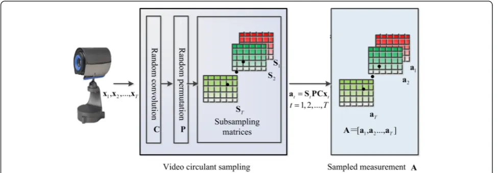
The authors of [16] have proposed a three-dimensional circulant sampling method, as shown in Figure 1, which can perform video sensing and compression simultan-eously with low computational complexity and easy hardware implementation. This method achieves video compression in two steps: the first step is random con-volution, which yields circulant measurements Cxt through convolving the original vectorized video frames
xt(t= 1, 2,…,T) with a circulant matrix C. The second step is random subsampling, which aims to reduce the number of circulant measurements Cxt. In this step, a random permutation is first applied to each vector Cxt by a permutation matrix P. Then the permuted vectors (measurements) PCxt are each subsampled utilizing a subsampling matrix St to generate the compressed (di-mension-reduced) measurements at=StPCxt. In the figure, the whole compressed measurements are denoted by matrixA= [a1,a2…,aT].
Given the sampled measurement matrixA, how to re-construct the foreground and background becomes a key problem in the CS-based object detection. In 2009, Candes et al. proposed a robust principal component analysis (RPCA) model to simultaneously reconstruct the video foreground and background by solving the fol-lowing minimization problem:
min
B;F k kB þ λk kF 1 s: t: X ¼ B þ F ð1Þ whereX ∈R(MN) ×T is the original video sequence, and
(2) In RPCA, the foreground reconstruction result is robust only to the corruption that has a sparse distribu-tion [17,18]. In the real-world video sequence, however, there rarely exists the movement turbulence that is sparse in nature.
The so-called three-dimensional total variation (TV3D) has recently been proposed for CS-based video reconstruction [16], which can exploit both intra-frame and inter-frame correlations of the video sequence. The advantage ofTV3Dis that it can guarantee the perform-ance of video reconstruction result with a low computa-tional complexity (O(3 ×MN×T)). TheTV3Dmodel is formulated as:
TV3Dð Þ ¼X kD1Xk1þkD2Xk1þρkD3Xk1 ð2Þ
where D1 and D2 are, respectively, the horizontal and vertical difference operators within a frame, and D3 is the time-varying difference operator.
In order to detect the moving object from the sampled measurement directly, we propose a new object detec-tion model, by combining TV3D and RPCA, that can simultaneously reconstruct foreground, background, and video sequence. The proposed object detection model is described as:
min
B;F;XTV 3Dð Þ þX γrankð Þ þB ηk kF 1
s: t:ΦX¼A;X ¼BþF
ð3Þ
where X= [x1, x2, …, xT] represents the original video sequence to be reconstructed B= [b1, b2, …, bT] is the background,F= [f1, f2…, fT] is the foreground (moving object), andΦis the measurement matrix. Since the ac-curacy of the reconstructed background and foreground relies on the performance of the video reconstruction re-sult, the TV3D is used to enhance the quality of the
reconstructed video. As mentioned earlier, TV3D has a low computational complexity (see (2)), while (3) gives a similar computational complexity as RPCA does. There-fore, problem (3) is less insensitive to the variable initialization, and we can initialize X, B andF as zero matrices. Note that solving the minimization problem of rank(B) in (3) is NP-hard due to its nonconvexity and discontinuous nature [17]. We would like to relax the rank(B) function through a nuclear norm, leading (3) to:
min B;F;X
X3
i¼1
aikDiXk1þγk kB þηk kF 1
s: t: ΦX ¼ A;X ¼ B þ F
ð4Þ
The difference between problem (4) and the 3DCS model in [16] is that: the 3DCS model is aimed to give a high video reconstruction result, where not only TV3D is used for video reconstruction but also the nuclear norm is adopted to make use of the low-rank property of the video sequence in the wavelet domain. Problem (4) in this paper is, however, aimed to exactly recon-struct the video foreground and background using a small number of sampled measurements. To achieve this goal, we employ TV3Dto guarantee the exact low-rank and sparse decomposition.
element of O is 0 or 1. We then use O to further im-prove the reconstructed foreground F^ through ⊙ F^, where ⊙ denotes the Hadamard (point-wise) product. Note that the confidence map is a binary matrix, in which the location of the movement turbulence is set to 0 and the location of the moving object is set to 1.
In real-world video surveillance, movement turbulence is repetitive and locally centered [20,21], which can be modeled by Gaussian distribution [22,23]. In this paper, we utilize the following mixed Gaussian model to esti-mate the intensity distribution of a pixel undergoing movement turbulence [22].
f xij ¼ωf1xij;μx;σxþð1−ωÞf2 xij;μp;Σp
ð5Þ
wheref(xij) represents the probability density of a pixel
xijatjth element in theith column of X^,ωis the weight of the two Gaussian models,μxandσxare the mean and the standard deviation, which are estimated by the EM algorithm, andμpandΣpare the mean and the covari-ance matrix, which are estimated from the particle tra-jectory of xij [22]. Particle trajectory aims to capture the deformation caused by movement turbulence, which can be obtained by using Lagrangian particle trajectory advection approach [24,25].
The confidence map is obtained as follows: we first es-timate each pixel’s probability density f(xij) using (5), then we decide which pixels belong to the movement turbulence and which ones belong to the moving object using an threshold θ. If f(xij) >θ, we set it as 1. Other-wise, we set it as 0. The obtained binary matrix is the final confidence map.
3 Reconstruction algorithm
In problem (4), we generalize the process of video compres-sion asat=Φxt. Since we use P,C, and St(t= 1, 2,…,T) to generate the compressed measurementA(see Figure 1), we should use the specific form rt=Cxt and StPrt=at
Next, we propose an alternating algorithm for the re-construction ofX,B, andF in (6). Each iteration of the alternating algorithm contains two steps: R-step, which aims at reconstructing the original video X; and S-step, which is to segment background and foreground.
In R-step, we reconstruct X by solving the following problem:
We adopt the augmented Lagrange multiplier (ALM) algorithm [26] to solve problem (7). The augmented Lagrange function of (7) is given by:
ℒðX;Gi;R;λi;υÞ ¼
where λi and υ are Lagrange multiplier matrices. The constrained optimization problem in (7) has been re-placed by problem (8). The ALM algorithm is to solve the minimization problem of (8) by iteratively minimiz-ing the Lagrange function and updatminimiz-ing the Lagrange multiplier,
Note that it is difficult to solve (9) directly. One can use an alternating strategy to minimize the augmented Lagrange function with respect to each component sep-arately, namely,
The sub-problem in (12) is solved as follows:
where Sα(·) is a soft-thresholding operator, which is
defined, for a scalarx, as:
Sαð Þ ¼x sign xð Þ⋅max xfj j−α;0g ð16Þ
where α is represented as a soft-thresholding. Suppose there is a matrix Z= (zij). Then, Sα(Z) outputs a matrix
which defines an operator for matrix Z with respect to scalar α, i.e., the elements ofSα(Z) follow the definition in (16).
Next, we solve the sub-problem (13) through the fol-lowing two steps [16].
rkþ1
t ¼Cxkt ðt¼1;2;…;TÞ ð17Þ
rkþ1
t ðPicStÞ ¼at ðt¼1;2;…;TÞ ð18Þ where PicSt is the index of measurements which is selected bySt, andrtis thetth column inR.
In sub-problem (14), X is updated through solving a quadratic problem.
By fixing Xk + 1, we reconstruct Band F in S-step by solving the following problem:
min
B;F γk kB þηk kF 1s:t:X
kþ1¼BþF ð19Þ
The augmented Lagrange function of (19) can be expressed as:
ℒðF;B;YÞ ¼k kB þηk kF 1þ<Xkþ1−B−F;Y
>þβ5 2 X
kþ1−B−F
2
F ð20Þ
whereYis the Lagrange multiplier matrix, and < ·, · > de-notes the matrix inner product. We use ALM algorithm to solve the minimization problem in (20) by the follow-ing two steps:
Fkþ1;Bkþ1
¼arg min
F;B ℒðF;B;YÞ ð21Þ Ykþ1¼YkþμXkþ1−Bkþ1−Fkþ1 ð22Þ
Similarly, we use an alternating strategy to minimize problem (21) with respect to each component separately:
Fkþ1¼arg min F ℒ F;B
k;Yk
ð23Þ
Bkþ1¼arg min B ℒ B;F
kþ1;Yk
ð24Þ
The complete algorithm proposed to solve problem (6) is summarized in Algorithm 1 below.
In the above algorithm, M¼X
3
i¼1
αiβiDT
i Diþβ4CTC,
Dα(·) is the singular value shrinkage operator [27], which is defined as follows: suppose the SVD of a matrixZ is given by Z=UΣVT, where Σ is an rectangular diagonal matrix in which each diagonal entries Σiiis the singular value ofZ,UandVare real unitary matrix. The singular value shrinkage operator for matrix Z is defined as Dα
Z
ð Þ ¼USαð ÞΣ VT, where Sα(·) is soft-thresholding
termination criterion is set as X
ering that the reconstruction of Band F rely on the re-construction ofX.
The solution to problem (7) does not guarantee a glo-bal minimum solution for problem (6). Moreover, it is difficult to rigorously prove the convergence of the pro-posed alternating algorithm for problem (7). But we can prove that there exists a feasible solution forX,B, andF that can minimize the cost function in (6). This feasible solution is stated in the following theorem.
Theorem 1: The sequence {Xk}, {Bk}, and {Fk} gener-ated in Algorithm 1 are bounded, and there exists a feas-ible point (X*,B*,F*) for the solution of problem (6).
The proof of Theorem 1 is given in Appendix.
4 Experimented results
In this section, we perform numerical experiments to show the performance of the proposed object detection algorithm. We focus on the illustration of the moving object reconstruction result and show that the new ob-ject detection algorithm is robust to the movement turbulence.
For quantitative evaluation, we utilize F-measure to evaluate the accuracy of the moving object detection re-sult. TheF-measure is defined as:
F‐measure¼2ðprecisionrecallÞ
precisionþrecall ð25Þ
where‘precision’and‘recall’are given by:
precision¼ TP
TPþFP;recall¼ TP
TPþFN ð26Þ
‘Precision’ and ‘recall’ are two kinds of classification accuracy parameters which are widely used to measure the accuracy of the background subtraction result [28]. In the ‘precision’ and ‘recall’, TP, FP, and FN are the number of true positives, the number of false positives, and the number of false negatives, respectively. The higher the F-measure, the better the accuracy of the moving object detection is. The major parameters used in Algorithm 1 are shown in Table 1. In our experi-ments, we compare the proposed object detection algo-rithm with the RPCA method as well as a widely used background subtraction algorithm called improved Guassian mixture model (GMM) [29]. Both RPCA and
GMM are operated in the spatial domain. All the experi-ments are performed on an Acer PC (CPU is Inter(R) Core(TM) i3-2310 M 2.10 GHz).
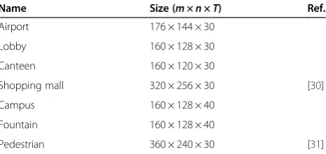
The testing video sequence for all the experiments are chosen from the database which are detailed in Table 2.
4.1 The new object detection model
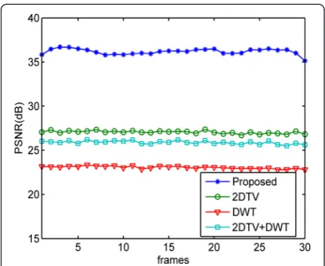
Here, we choose Fountain sequence as an example to show first the video reconstruction result of the new ob-ject detection model. In this experiment, we compare the video reconstruction result of the proposed object detection model with three known video reconstruction sparsity measures: 2DTV, DWT, and 2DTV + DWT. The simulation results in terms of peak signal-to-noise ratio (PSNR) of the four methods are shown in Figure 2.
It is seen that the PSNR of the reconstructed video using the proposed object detection model is signifi-cantly higher than that of 2DTV, DWT, and 2DTV + DWT. Figure 3 shows the twentieth frame of the original video sequence and the corresponding reconstruction results of the four methods. Evidently, the reconstructed video frame using the proposed object detection model is clearer than that from 2DTV, DWT, and 2DTV + DWT. We can conclude from this experiment that the proposed reconstruction model is able to yield superior video reconstruction performance.
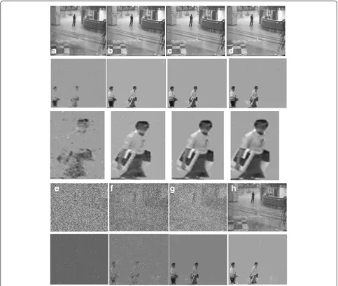
Next, we illustrate the video reconstruction and object detection results of our proposed model versus the sam-pling rate as shown in Figure 4. The chosen video se-quence is from an airport video which contains a large amount of edge information and thus can highlight the difference of video foreground reconstruction results at different sampling rates. In addition, we compare our object detection results with compressive principal com-ponent pursuit (PCP) in Figure 4, which clearly shows the advantage of using TV3Dnorm in our object detec-tion model.
Clearly, Figure 4b,c,d give an exact foreground recon-struction result, where in order to see the difference among three images, we have given the local magnified images of the foreground reconstruction result. It is seen that Figure 4d gives the best foreground reconstruction
Table 1 Parameters used in solving the proposed reconstruction model
Table 2 Sequence information used in experiments
result. Figure 4c gives a slightly better performance than Figure 4b does. This is because the sampling rate used in Figure 4c is higher than that in Figure 4b. Figure 4a does not give a clear foreground reconstruction result due to the poor performance of the video reconstruction result. Comparing with Figure 4a,b,c,d, Figure 4e,f,g,h give poor video foreground and background reconstruc-tion results. This is because that Figure 4e, f, g, h are re-constructed by compressive PCP, which is a special case of problem (6) when αi= 0 (i= 1, 2, 3). In this special case, the poor video reconstruction performance has be-come the bottleneck that precludes good video back-ground and foreback-ground reconstruction at low sampling rate. We can conclude from this experiment that using
TV3D norm in our model can guarantee a high object detection performance at low sampling rate. In addition to the above subjective measure of the object detection performances at different sampling rates, we choose PSNR and root mean square error (RMSE) as objective evaluation parameters to further illustrate the perform-ance of the proposed object detection model and com-pressive PCP at different sampling rates.
In Table 3, PSNR is used to measure the video recon-struction result and RMSE_B is utilized to evaluate the
RMSE of the background reconstruction result. From Figure 4 and Table 3, we could see that at 20% sampling rate, the PSNR of our video reconstruction result is already above 30 dB, this means that we have obtained enough information for the exact foreground recon-struction result.
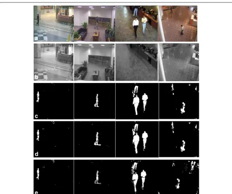
4.2 The moving object detection result
Here, we illustrate the performance of the proposed object detection algorithm with an emphasis on the reconstruc-tion of foreground and background. In order to compare with GMM algorithm, we give the binary form of our fore-ground reconstruction result in the following experiments. We choose four indoor video sequences (airport, lobby, canteen, and shopping mall) to illustrate that the proposed object detection algorithm is able to give a similar per-formance as the popular spatial-domain moving object de-tection methods do. The reconstruction results of our proposed algorithm for four indoor video sequences are shown in Figure 5, where columns 1 to 4 are the moving object detection results of airport, lobby, canteen, and shopping mall video sequences, respectively. It is seen that our proposed algorithm using only 20% sampled measure-ment can give a similar moving object detection perform-ance as the RPCA and GMM methods do. In the lobby and canteen video sequences, the proposed moving object detection algorithm is able to reduce the shadow turbu-lence. Table 4 gives objective evaluation results in terms of the F-measure of the proposed algorithm along with the two known methods for the four video sequences. We can see that the F-measure of the proposed object detection algorithm is obviously higher than that of the GMM method. From this experiment, we can conclude that the proposed moving object detection algorithm is able to exactly detect the moving object using only 20% sampled measurements in the indoor video sequences.
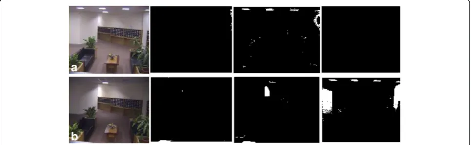
Figure 6 shows object detection results of the lobby video sequence with a sudden illumination change from the 10th frame to 11th frame. It is clearly seen that the proposed algorithm is robust to the sudden illumination changes of the indoor video sequence.
We now illustrate the performance of the proposed al-gorithm in outdoor video sequence. The outdoor video Figure 2PSNR performance at sampling rate 40%.
sequence usually contains strong movement turbulence. We choose campus, fountain, and pedestrian video quences for this experiment. The pedestrian video se-quence is captured by a COTS camera (the SONRY DCW-TRV 740).
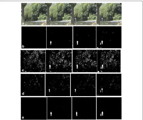
This test case is very challenging because the whole video sequence is strongly disturbed by the swaying tree and flag. From Figure 7, it is obvious that the proposed al-gorithm is able to effectively eliminate the turbulence of the swaying trees (Figure 7b), while RPCA is not robust to this kind of strong movement turbulence (Figure 7c). The post-processing result of RPCA (Figure 7e) can give a slightly better performance than the proposed algorithm does. Although the GMM method can reduce the
movement turbulence (Figure 7d), its foreground recon-struction result is not better than that of the proposed ob-ject detection algorithm. We can conclude from this experiment that the proposed object detection algorithm is able to give a robust foreground reconstruction result using only 40% sampled measurement.
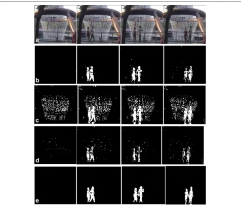
In this experiment, the background involves a huge fountain, which would strongly disturb the moving object. It is seen from Figure 8 that the new object detection algo-rithm is able to efficiently eliminate the fountain turbu-lence, and it gives a better foreground reconstruction result than the GMM method does (Figure 8b,d). RPCA is still not robust to this kind of movement turbulence (Figure 8c). The post-processing result of RPCA (Figure 8e) Figure 4The object detection performances at different sampling rate. (a)The background first row and foreground second row
Table 3 Evaluation of the proposed model at different sampling rate
Sampling rate 0.1 0.2 0.3 0.4 0.5 0.6 0.7 0.8
Proposed object detection model
PSNR 24.06 31.81 34.20 36.77 40.37 43.61 46.35 49.45 RMSE_B in RPCA
dB dB dB dB dB dB dB dB
RMSE_B 0.080 0.061 0.059 0.057 0.052 0.049 0.047 0.046
Compressive PCP
PSNR 4.61 5.16 6.83 7.19 7.32 12.51 22.43 30.56 Model is 0.045
dB dB dB dB dB dB dB dB
RMSE_B 0.924 0.828 0.632 0.577 0.522 0.292 0.130 0.079
is better than the proposed algorithm due to the fact that RPCA is operated in the spatial domain. The original video sequence can give RPCA a large amount of detailed information.
We choose a real-world outdoor video sequence to conduct this experiment. The chosen video sequence contains ordinary turbulence such as shadow and cam-eral noise. We randomly select four frames to show the moving object detection performance of different methods. It is clearly shown in Figure 9b that the pro-posed object detection algorithm is able to exactly distinguish the contour outlines of the moving per-son. It can completely eliminate the cameral noise. Both of RPCA and GMM (see Figure 9c,d) could not give a clear moving object detection result. The aver-aged F-measure of Figures 7, 8, and 9 are given in Table 5, which show that the proposed algorithm gives an obviously higher F-measure than the RPCA and GMM methods do.
5 Conclusion
In this paper, we have proposed a CS-based algorithm for detecting the moving object in video sequences. In order to achieve robust foreground reconstruction result using only a small number of sampled measurements, we have first proposed an object detection model to sim-ultaneously reconstruct the foreground, background, and
the original video sequence using the sampled measure-ments. Then, the reconstructed video sequence is used to estimate a confidence map to refine the foreground reconstruction result. It has been shown through experi-ment that the proposed moving object detection algo-rithm can give a good performance for both indoor and outdoor video sequences. Especially for outdoor video sequence, the proposed reconstruction model is able to effectively eliminate the movement turbulence such as waving trees, water fountain, and video noise. In conclu-sion, the proposed moving object detection algorithm can achieve an accuracy comparable to some known spatial-domain methods with a significantly reduced number of sampled measurements. The limitation of the proposed method includes: (1) In Algorithm 1, solving nuclear norm imposes high computational complexity. (2) There is a lack of theoretical analysis of the impact of the sampling rate on the object detection result. To solve those problems in future work, (1) we will use an online version of object detection model to achieve background reconstruction, and (2) we will refer to [15] for possible theoretical analysis of the performance of the proposed model.
6 Appendix: Proof of Theorem 1
The proof of Theorem 1 is based on following two Lemmas.
Lemma 1: Let aki ¼λki−τ Gkiþ1−DiXk
i¼1;2;3
ð Þ,
bk=Yk+μ(Xk+ 1−Bk+ 1−Fk)ck=Yk+μ(Xk+ 1−Bk+ 1− Fk + 1
). The sequence aki ði¼1;2;3Þ, {bk} and {ck} are bounded.
Proof of Lemma 1
(i) We prove first aki ði¼1;2;3Þis bounded.
In each iteration of Algorithm 1,Gi, (i= 1, 2, 3) is up-dated through solving problem (7), and B and F are Table 4 Quality evaluation (F-measure) of the detection
results in Figure 5
Sequence Proposed RPCA GMM
Airport 0.55 0.56 0.50
Lobby 0.56 0.45 0.43
Canteen 0.63 0.61 0.59
Shopping mall 0.49 0.50 0.39
reconstructed through solving problem (19). When min-imizing the Lagrange function in (8), we can obtain:
Gkþ1
i ¼minGiℒ Gi;Rk;Xk;λki;υk
⇒0∈∂Giℒ Gkþi 1;Rk;Xk;λki;υk
⇒ak
i∈∂Gi G kþ1 i
1ði¼1;2;3Þ ∵ ak
i∈∂GiGkiþ11, hence, a
k
i ði¼1;2;3Þis bounded
[22].
(ii) Now we prove {bk} and {ck} are bounded.
When minimizing the Lagrange function in (20), we can obtain that:
Bkþ1 ¼min
BℒB;Fk;Yk
⇒0∈∂BℒBkþ1;Fk;Yk
⇒bk∈∂
BBkþ1
∵bk∈ ∂
B‖Bk+ 1‖*, so the sequence {bk} is bounded [22].
Fkþ1 ¼min
FℒBkþ1;F;Yk
⇒0∈∂FℒBkþ1;Fkþ1;Yk
⇒ck∈∂
F Fkþ1 1
∵ck∈ ∂
F‖Fk+ 1‖1, hence the sequence {ck} is bounded [22].
Lemma 2: Letℒ(B, F,Y) be the Lagrange function of problem (19). Then we haveℒk+ 1=ℒ(Bk+ 1,Fk+ 1,Yk) andℒkþ1−ℒk≤1μek withek=‖Yk−Yk−1‖F,k= 1, 2,…
Proof of Lemma 2
Letℒk+ 1=ℒ(Bk+ 1,Fk+ 1,Yk), then:
ℒkþ1≤LBk;Fk;Yk¼ Bk
þη1 Fk 1þ X
k−Bk−Fk;Yk
þβ5 2 X
k−Bk−Fk
2
F¼ℒkþ<Xkþ1−Bk−Fk;Yk−Yk−1> ðA1Þ
Yk ¼Yk−1þμXkþ1−Bk−Fk⇒Yk−Yk−1
μ
¼Xkþ1−Bk−Fk ðA2Þ
Substituting (A2) into (A1), we can obtain that ℒkþ1−
ℒk≤1
μYk−Yk−1F. End of proof of Lemma 2.
In Algorithm. 1, we need to solve two Lagrange func-tions: ℒ(X, Gi, R, λi, υ) and ℒ(B, F, Yk) for the recon-struction of X, B andF. If there exists a feasible point (X*, B*, F*) for the solution of problem (6), we must make sure thatℒ(X,Gi,R,λi,υ) andℒ(B,F,Yk) are all bounded.
In Theorem 1 of [16], it has been proved that ℒ(X,
Gi, R, λi, υ) is bounded, so we only need to prove that
ℒ(B, F, Yk) is bounded. We have proved that: {ck} is bounded in Lemma 1.
Noting thatYk+ 1=ck, we have bounded {Yk}.
Since ℒkþ1−ℒk≤1μYk−Yk−1F and {Yk} is bounded, we conclude thatℒ(B,F,Yk) is bounded.
Next we prove that {Xk}, {Bk} and {Fk} are bounded. As it has been proved thatℒ(X, Gi,R,λi,υ) is bounded, we can obtain that the Lagrange multiplier λki is bounded.
From (10) in paper, we obtain:
λkþ1
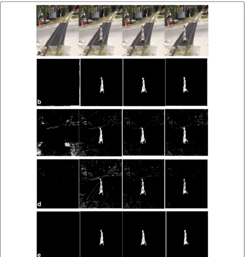
i ¼λki−τGkþi 1−DiXkþ1 ðA3Þ Figure 9Object detection results of pedestrian video sequence. (a)Original video sequence.(b)Reconstructed foreground using the proposed algorithm.(c)Reconstructed foreground using RPCA.(d)Reconstructed foreground using GMM.(e)Reconstructed foreground using modified RPCA (the manual postprocess result of RPCA). The sampling rate of our algorithm is 40% and four frames, i.e., 1st, 8th, 12th, and 15th frame are randomly selected.
Table 5 Quality evaluation (F-measure) on Figures 7, 8, and 9
Experiments Proposed RPCA GMM Modified RPCA
Figure6 0.36 0.07 0.13 0.38
Figure7 0.49 0.18 0.47 0.55
From Lemma 1, we have:
λk
i ¼aki þτGikþ1−DiXk ðA4Þ
Subtracting (A4) into (A3), we get:
λkþ1
F converge to 0, we can prove that
{Bk} and {Fk} are bounded.
Competing interests
The authors declare that they have no competing interests.
Acknowledgements
This work was supported by the National Natural Science Foundation of China (No.61372122 and 61302103); the Innovation Program for Postgraduate in Jiangsu Province under Grant (No. CXZZ13_0491).
Author details
1College of Communication and Information Engineering, Nanjing University
of Posts and Telecommunications, Nanjing 210003, China.2Department of Electrical and Computer Engineering, Concordia University, Montreal, QC H3G 1 M8, Canada.
Received: 17 August 2014 Accepted: 5 January 2015
References
1. O Barnich, M Van Droogenbroeck, ViBe: a universal background subtraction algorithm for video sequences. IEEE Trans. Image Process.20(6), 1709–1724 (2011)
2. Brutzer, B Hoferlin, G Heidemann, Evaluation of background subtraction techniques for video surveillance, inIEEE Conference on Computer Vision and Pattern Recognition (CVPR), 2011, pp. 1937–1944
3. T Du-Ming, L Shia-Chih, Independent component analysis-based background subtraction for indoor surveillance. IEEE Trans. Image Process.18(1), 158–167 (2009)
4. Z Baochang, G Yongsheng, Z Sanqiang, Z Bineng, Kernel similarity modeling of texture pattern flow for motion detection in complex background. IEEE Trans. Circuits Syst. Video Technol.21(1), 29–38 (2011)
5. K Wonjun, K Changick, Background subtraction for dynamic texture scenes using fuzzy color histograms. IEEE Signal Process. Lett.19(3), 127–130 (2012) 6. S Chen, J Zhang, Y Li, J Zhang, A hierarchical model incorporating
segmented regions and pixel descriptors for video background subtraction. IEEE Trans Ind Inf.8(1), 118–127 (2012)
7. H Bohyung, LS Davis, Density-based multifeature background subtraction with support vector machine. IEEE Trans. Pattern Anal. Mach. Intell. 34(5), 1017–1023 (2012)
8. R Baraniuk, Compressive sensing. IEEE Signal Process. Mag.24(4), 118–121 (2007) 9. DL Donoho, Compressed sensing. IEEE Trans. Inf. Theory52(4), 1289–1306 (2006) 10. EJ Candes, MB Wakin, An introduction to compressive sampling. IEEE Signal
Process. Mag.25(2), 21–30 (2008)
11. J Ma, G Plonka, MY Hussaini, Compressive video sampling with approximate message passing decoding. IEEE Trans. Circuits Syst. Video Technol.22(9), 1354–1364 (2012)
12. V Cevher, A Sankaranarayanan, M Duarte, D Reddy, R Baraniuk, R Chellappa, Compressive sensing for background subtraction, inPro. European Conference on Computer Vision (ECCV), 2008
13. H Jiang, W Deng, Z Shen, Surveillence video processing using compressive sensing. Inverse Probl. Imaging6(2), 201–214 (2012)
14. F Yang, H Jiang, Z Shen, W Deng, D Metaxas, Adaptive low rank and sparse decomposition of video using compressive sensing, in Proc. IEEE International Conference on Image Processing (ICIP), 2013, pp. 1016–1020
15. J Wright, A Ganesh, K Min, Y Ma, Compressive principal component pursuit. Inf. Inference2(1), 32–68 (2013)
16. X Shu, N Ahuja, Imaging via three-dimensional compressive sampling (3DCS), inIEEE International Conference on Computer Vision (ICCV), 2011, pp. 439–446
17. B Bao, G Liu, C Xu, S Yan, Inductive robust principal component analysis. IEEE Trans. Image Process.21(8), 3794–3800 (2012)
18. EJ Candes, X Li, Y Ma, J Wright, Robust principal component analysis? J. ACM58(1), 1–37 (2009)
19. E Borenstein, E Sharon, S Ullman, Combining top-down and bottom-up segmentation, inProc. Conference on Computer Vision and Pattern Recognition Workshop, 2004, p. 46
20. M Shimizu, S Yoshimura, M Tanaka, M Okutomi, Super-resolution from image sequence under influence of hot-air optical turbulence, in Proc. IEEE Conference on Computer Vision and Pattern Recognition (CVPR), 2008, pp. 1–8
21. O Oreifej, G Shu, T Pace, M Shah, A two-stage reconstruction approach for seeing through water, inIEEE Conference on Computer Vision and Pattern Recognition (CVPR), 2011, pp. 1153–1160
22. O Oreifej, X Li, M Shah, Simultaneous video stabilization and moving object detection in turbulence. IEEE Trans. Pattern Anal. Mach. Intell. 35(2), 450–462 (2013)
23. C Stauffer, WEL Grimson, Adaptive background mixture models for real-time tracking, inIEEE Computer Society Conference on Computer Vision and Pattern Recognition, vol. 2, 1999, p. 252
24. W Shandong, O Oreifej, M Shah, Action recognition in videos acquired by a moving camera using motion decomposition of Lagrangian particle trajectories, inIEEE International Conference on Computer Vision (ICCV), 2011, pp. 1419–1426
25. S Wu, BE Moore, M Shah, Chaotic invariants of Lagrangian particle trajectories for anomaly detection in crowded scenes, inIEEE Conference on Computer Vision and Pattern Recognition (CVPR), 2010, pp. 2054–2060 26. W Yin, S Morgan, J Yang, Y Zhang, Practical compressive sensing with
Toeplitz and circulant matrices, inVisual Communications and Image Processing Huangshan China, 2010
27. H Yao, Z Debing, Y Jieping, L Xuelong, H Xiaofei, Fast and accurate matrix completion via truncated nuclear norm regularization. IEEE Trans. Pattern Anal. Mach. Intell.35(9), 2117–2130 (2013)
29. Z Zivkovic, Improved adaptive Gaussian mixture model for background subtraction. Int. Conf. Pattern Recog.2, 28–31 (2004)
30. L Li, W Huang, IYH Gu, Q Tian, Statistical modeling of complex backgrounds for foreground object detection. IEEE Trans. Image Process.13(11), 1459–1472 (2004) 31. Y Sheikh, M Shah, Bayesian modeling of dynamic scenes for object
detection. IEEE Trans. Pattern Anal. Mach. Intell.27(11), 1778–1792 (2005)
Submit your manuscript to a
journal and benefi t from:
7Convenient online submission
7Rigorous peer review
7Immediate publication on acceptance
7Open access: articles freely available online
7High visibility within the fi eld
7Retaining the copyright to your article