R E S E A R C H
Open Access
Asymptotic BER EXIT chart analysis for
high rate codes based on the parallel
concatenation of analog RCM and digital
LDGM codes
Imanol Granada
1*, Pedro M. Crespo
1and Javier Garcia-Frías
2Abstract
This paper proposes an extrinsic information transfer (EXIT) chart analysis and an asymptotic bit error rate (BER) prediction method to speed up the design of high rate RCM-LDGM hybrid codes over AWGN and fast Rayleigh channels. These codes are based on a parallel concatenation of a rate compatible modulation (RCM) code with a low-density generator matrix (LDGM) code. The decoder uses the iterative sum-product algorithm to exchange information between the variable nodes (VNs) and the two types of constituent check nodes: RCM-CN and LDGM-CN. The novelty of the proposed EXIT chart procedure lies on the fact that it mixes together the analog RCM check nodes with the digital LDGM check nodes, something not possible in previous multi-edge EXIT charts proposed in the literature.
Keywords: Rate compatible modulation (RCM), Low-density generation matrix (LDGM), EXIT charts, BER prediction, Joint source-channel coding (JSCC)
1 Introduction
We propose an extrinsic information transfer (EXIT) chart analysis and an asymptotic bit error rate (BER) pre-diction method to speed up the design of high rate (greater than 2 bits per complex channel symbol) RCM-LDGM hybrid channel codes for the transmission of memory-less binary sources over additive white Gaussian noise (AWGN) and fast Rayleigh channels. These hybrid codes consist of the parallel concatenation of a rate compatible modulation (RCM) code (see, e.g., [1,2]) and a low-density generator matrix (LDGM) code (see, e.g., [3,4]). In what follows, we will refer to these schemes as parallel RCM-LDGM codes. Both uniform and non-uniform sources are considered. The reason for considering non-uniform sources is that many data sources (e.g., image or speech signals) are non-uniformly distributed, containing sub-stantial amount of natural redundancy [5–8]. Even when these sources are compressed, they still exhibit a residual
*Correspondence:[email protected]
1Department of Basic Science, University of Navarra, Mikeletegi Pasealekua, 48, 20018 San Sebastian, Spain
Full list of author information is available at the end of the article
redundancy due to the sub-optimality of the compression scheme [9].
RCM codes generate random projections (RP) from weighted linear combinations and are able to achieve smooth rate adaptation in a broad dynamic range. How-ever, they present error floors at high signal to noise ratios (SNRs). In order to solve this drawback, [10, 11] sug-gested the use of an LDGM code in parallel with the RCM code, aiming at reducing the error floor. Simula-tion results in [10,11] show that the parallel RCM-LDGM code outperforms RCM schemes significantly, achieving a performance close to the Shannon limit if suitable design parameters are chosen.
One of the main advantages of this class of high rate RCM-LDGM codes over other high rate codes, such as the widely adopted bit-interleaved coded modulation (BICM) [12], is the easiness of performing adaptive coded mod-ulation (ACM). Conventional ACM is done by selecting the best combination of channel coding and modulation based on the estimated channel condition. Due to the limited number of rate combinations, a stair-shaped rate curve is often obtained. Moreover, ACM requires instant and accurate channel estimation. Due to their intrinsic
design, RCM codes are well suited to overcome these adaptation challenges (refer to [2] for a comparison with other ACM schemes). The reason is that their coded symbols are generated by a set of weighted linear com-binations of the source binary symbols. By varying the number of linear combinations on a per symbol basis, a smooth rate adaptation is possible.
Another advantage of RCM-LDGM codes is in the transmission of non-uniform memoryless sources. Existing low rate joint source-channel coding schemes [7,8,13,14] present a gap to the Shannon theoretical limit of about 2 dB for sources with low non-uniformity. How-ever, this gap increases when the source becomes more non-uniform, i.e., when its entropy decreases. Unlike these low rate joint source-channel codes, it is shown in [11] that RCM-LDGM codes are able to maintain the gap to the theoretical limit as the non-uniformity increases, while keeping very large throughputs. Their robustness against channel and source variations, together with the fact that smooth rate adaption is possible, makes RCM-LDGM codes excellent candidates in applications where channel and source variations are encountered. However, the proposed RCM-LDGM codes found in the literature [10, 11], have been designed by a trial-error procedure, something that requires a large amount of simulation time. Here, to circumvent this design drawback, we pro-pose an EXIT chart analysis that facilitates the selection of suitable code parameters.
EXIT charts were first introduced in [15] to analyze and design an iterative coding scheme. Later, [16] pro-posed a curve fitting procedure based on EXIT charts to design a low-density parity check (LDPC) code valid for modulation and detection. Due to the iterative decoding nature of parallel RCM-LDGM codes, EXIT charts are a good method to visually explore the iterative exchange of information that occurs in the decoders of these schemes. The authors in [17] were the first to use EXIT charts as a design aid for pure RCM codes. However, the EXIT
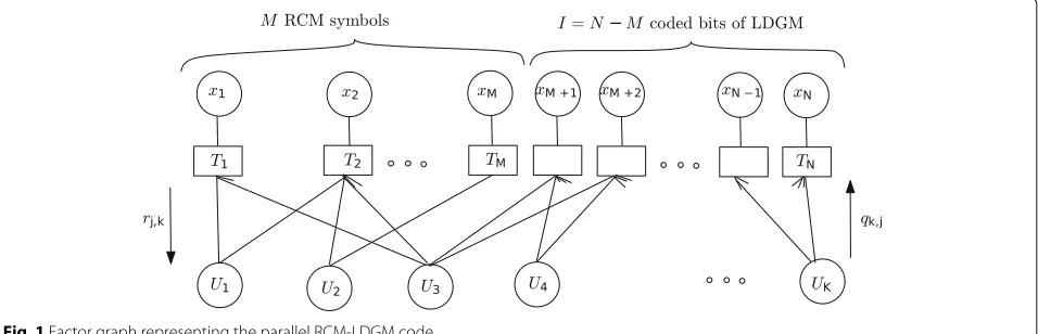
analysis for pure RCM codes is not valid in our case, since two different types of check nodes, RCM and LDGM, have to be considered (refer to Fig.1). EXIT chart analysis con-sidering multiple edge node types has been extensively investigated in the literature, e.g., in [18] multi-edge type EXIT charts are used to design the bit mapping for LDPC coded BICM schemes, and in [19], EXIT charts are used to optimize the bit mapping of LDPC coded modulation with APSK constellations. Irregular LDPC codes are also exam-ples of EXIT charts with different check nodes. However, RCM-LDGM codes present the added difficulty of mixing analog and digital check nodes, and therefore, previous strategies cannot be directly applied.
The contribution of this paper is twofold:
1 Developing an EXIT chart analysis that is able to deal with the check node disparity encountered in parallel RCM-LDGM codes when driven by binary
memoryless sources (both uniform and
non-uniform) transmitted over AWGN and fast fading Rayleigh channels
2 Assessment of the time savings achieved by using the EXIT chart analysis, rather than Monte Carlo simulations, for BER predictions
The remainder of the paper is organized as follows. Section2briefly reviews previous work on the design of
RCM and parallel RCM-LDGM codes. Section3presents
the proposed EXIT chart analysis and BER prediction
for RCM-LDGM codes. Section4evaluates the proposed
EXIT chart-BER prediction method, comparing the
pre-dicted BER with simulation results. Finally, Section 5
concludes this paper.
2 Background: RCM and RCM-LDGM code design
Consider a point-to-point communication system where a binary memoryless source with distribution(p0;p1 = 1−p0)transmitsKbitsu=(u1,u2,. . .,uK)∈ {0, 1}K×1,
across an AWGN channel, to a far end receiver. To that end, the source symbolsuare encoded by a rateR=K/N
(bits per real dimension) parallel RCM-LDGM encoder and quadrature amplitude modulation (QAM) modulated before being transmitted. Let
x=(x1+ix2,x3+ix4,. . .,xN−1+ixN)
be the sequence of N/2 complex baseband modulated
symbols to be transmitted, where xi ∈ R denotes the
coded symbols at the output of the RCM-LDGM encoder.
Assuming independence of the coded symbols {xi}, a
set of sufficient statistics to estimate u is given by the output of an equivalent discrete time AWGN channel
y=(y1,y2,. . .,yN)∈RN×1,
yi=xi+ni, i∈ {1, 2,. . .,N}
where {ni}Ni=1 are realizations of i.i.d real Gaussian ran-dom variables (RVs) with zero mean and varianceN0/2 (i.e.,Ni ∼N(0,N0/2)). At the receiver side, the decoder estimates the source symbolsufromy.
For the sake of clarity in the exposition, we begin by pro-viding a succinct overview of the key concepts of RCM and LDGM codes before covering parallel RCM-LDGM codes.
2.1 Rate compatible modulation (RCM) codes
An RCM code of rateK/Mbits per real dimension is char-acterized1by an M×K sparse generator matrixG. Let D⊂ Nbe a multiset2withd(RCMc) /2 elements whereNis the set of natural numbers (positive integers). The entries of Gbelong to±D. As an example, let d(RCMc) = 8 and assumeKto be divisible byd(RCMc) . Then, the construction of matrixGis given by the following steps:
1 Construct theK/2×KmatrixG0as
where(·)denotes random column permutations of a matrix, andDdl is aK/8×K/4sparse matrix given
2 Vertically stack as manyG0s as needed. Note that we should keep only as many rows as needed in the last
stackedG0matrix so that the requiredM×K G matrix is obtained.
Observe thatdRCM(c) gives the number of nonzero entries of any row of G. Similarly, we denote bydRCM(vk) ≥ 2 the number of nonzero entries of columnkof matrixG, and byd(RCMv) its average value, i.e,d(RCMv) = K1Kk=1d(RCMvk) .
2.2 Low-density generator matrix (LDGM) codes
Low-density generator matrix codes, or LDGM codes, are a binary class of codes with a sparse generator matrixGL. In this work, we will consider systematic LDGM codes, i.e., codes whose generator matrix is of the form GL = [IK|P], whereIK is the identity matrix of sizeKandPis aK×Isparse matrix. We will consider regular matrices
P, which are characterized by the pairdLDGM(v) ,dLDGM(c) , denoting the number of nonzero elements of a column and of a row, respectively. LDGM codes are a subclass of LDPC codes, where the parity check is given by the sparse matrixH =[P|II]. Since the generator matrix is sparse, the encoding of LDGM codes can be done in
lin-ear time and the codeword of lengthN = K+Ican be
written as
c=[c1,c2,. . .,cN]=uGL=u[IK|P]
=[u1,u2,. . .,uK,x1,x2,. . .,xI] ,
where in this case the operations are in the binary field. Although LDGM codes have the advantage of linear encoding complexity, unlike general LDPC codes, they can only attain an arbitrarily low error probability by reducing the rate to zero [20]: Independently of the block length, they suffer from a high error floor. Therefore, they have been historically disregarded in favor of other LDPC codes. However, as explained in the next section, they can actually perform well as an aid to reduce the error floor of other codes.
2.3 Parallel RCM-LDGM code
As shown in Fig.1, a parallel RCM-LDGM code of rate
K/(M+ I) bits per real dimension consists of the
par-allel concatenation of an RCM code of rate K/M with
a high rate binary regular LDGM code that produces I
binary symbols. That is, the encoded symbol sequence is
where G is the M × K RCM matrix introduced in
Section2.1andPis the non-systematic part of the LDGM generator matrix in Section2.2. Recall that the objective of the LDGM code is to reduce the error floor produced by the RCM code, but without degrading the RCM waterfall region.
As explained before, the RCM symbols and the BPSK modulated LDGM coded bits are grouped two by two and transmitted using a QAM modulator, so that the spectral efficiency,ρ, is
ρ= 2·K M+I
bits per complex channel symbol. In the results, we will utilize the spectral efficiency,ρ, instead of the rate (given by MK+I).
2.4 Decoder block
For decoding, the sum-product algorithm (SPA) [21] is applied to the factor graph that models the overall com-munications system. This factor graph is sketched in Fig. 1. Letrj,k andqk,j denote the passing log-likelihood ratio (LLR) messages from thejth check node (CN) to the
kth variable node (VN), and from thekth VN to thejth CN, respectively. In what follows, we denote byn(Uk)\Tj andn(Tj)\Ukthe set of CNs connected to VNUkwithout considering CNTj, and the set of VNs connected to CN
Tjwithout considering VNk, respectively. At each itera-tiont, the sum-product algorithm is implemented by the sequential execution of the following steps:
• Step 1.q(kt,)i: Message passing from variable nodes, (p1;p0)is the distribution of the memoryless binary source.
over alli except k. Combining both terms, we
getxj=aj,k+gj,kukfor allk∈n(Tj), and the
where the sum inz is over all possible values that the RCM symbols can take. Notice that P(t)(aj,k=z), the probability ofaj,k =zat
iterationt, is calculated in a straightforward manner by convolving the probability density functions (PDFs) of the terms in the
summation, where the distribution functions of these terms are obtained from the received LLR messagesq(kt,)i. An efficient way to
implement these convolutions is explained in [1]. – Computation at LDGM check nodes
{Ti}Mi=+MI+1: As in standard LDGM codes, the LLR message transmitted from thei th check node to the variable nodeUkis given by
r(i,tk)= −2atanh
At the end of the iterations, whent=tmax, an estimate ofukcan be calculated as
3 Methods: EXIT chart analysis for the LDGM-RCM code
nodes, RCM and LDGM, have to be considered. This paper extends the analysis to parallel RCM-LDGM codes, considering as well non-uniform sources. Furthermore, it also presents a BER prediction analysis based on EXIT charts that was not previously considered in the literature for this type of codes.
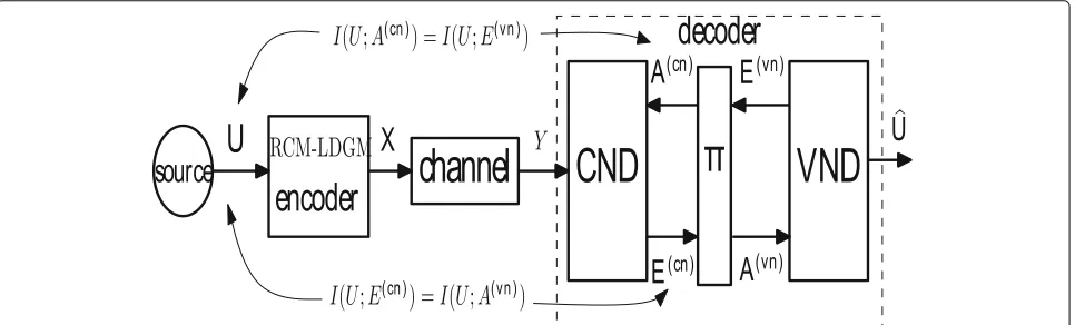
As shown in Fig.2, the model for EXIT chart analysis is composed of two types of decoders: variable node decoder (VND) composed of all variable nodes, and check node decoder (CND) composed of two different types of check nodes, RCM and LDGM working in the real and binary field, respectively. The LLR values exchanged between the two decoders are modeled as outcomes of real-valued ran-dom variablesE(output from either a VND or a CND) and
A(input to either a VND or a CND).
To characterize the behavior of a node decoder, either check or variable, we obtain the mutual information
I(E;U)between the decoder’sLLRextrinsic outputEand a binary source symbolUwith distribution(p1;p0), as a function of the mutual informationI(A;U) between the decoder’s LLR a priori inputAandU.I(E;U)andI(A;U)
are given by
I(L;U)=p0
∞
−∞fL(ξ|0)log2
fL(ξ|0)
p0fL(ξ|0)+p1fL(ξ|1))
dξ
+p1
∞
−∞fL(ξ|1)log2
fL(ξ|1)
p0fL(ξ|0)+p1fL(ξ|1))
dξ,
(5)
whereL ∈ {A,E}andfL(ξ|u), foru = 0, 1, is the condi-tional probability density function ofLgivenU. As indi-cated before,fL(ξ|u)depends on the node decoder under consideration, that is, whether such a node is a VND or a CND, and it is calculated as indicated in Sections3.1and
3.2. In the sequel, we will denote I(L;U) for a VND or
a CND as IL,VND = I
L(vn);Uor I
L,CND = I
L(cn);U, respectively.
In the course of deriving the EXIT chart for the parallel RCM-LDGM code, we will need the parameters
p(RCMvn) M·d
(v) RCM
M·d(RCMv) +I·d(LDGMv)
(6)
p(RCMcn) d
(c) RCM
d(RCMc) +d(LDGMc) , (7)
which denote the average percentage of edge connections arriving to a VN from an RCM check node and the per-centage of edge connections arriving to an RCM check node from a VN, respectively.
3.1 VND EXIT curve for RCM-LDGM codes
The EXIT curve of the VND is given by the trans-fer characteristic between IE,VND = I(E(vn);U) and IA,VND = I(A(vn);U). Note that the realizations of RVs E(vn) andA(vn) are the messages exchanged in the sum-product algorithm, {ri,k} and {qk,i}, respectively. In order to evaluate these mutual informations from (5), the conditional PDF of the a prioriA(vn)and the extrin-sic E(vn) at a variable node decoder, given U, have to be found.
3.1.1 Calculation ofIA,VND
Different from previous work on EXIT charts, in an RCM-LDGM code, one has to consider two types of a priori messages arriving at a VND: first, the mes-sages arriving from an edge connected to an RCM check node, A(RCMvn) , and second, the messages arriv-ing from an edge connected to an LDGM check node,A(LDGMvn) .
In order to simplify calculations, the authors in [17] modeled the conditional PDF of theA(RCMvn) message as the PDF of the LLR random variable obtained at the output of a virtual AWGN channel when its inputs are uniform3 binary source symbolsU, i.e.,
Y=U+N, N∼N0,σ2. (8)
Under this model, the LLR of the a priori messageA(RCMvn)
at a variable node can be expressed as
A(RCMvn) =log of the two different virtual channels.
The main challenge of having two different types of CNs rather than one, as in the case of a standard EXIT chart,
is that the mutual information IA,VND will now depend
on two variables,σ2
R,A andσL2,A, rather than just on one. Notice, however, that although A(RCMvn) |U and A(LDGMvn) |U
can be considered independent, their variances are cou-pled due to the way the SPA generates the messages (refer to Section2.4). Therefore, if one of the variances can be expressed as a function of the other, then IA,VND becomes a function of only one variable, which simplifies the analysis.
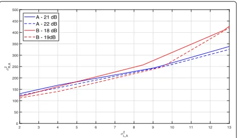
Calculating the coupling between σR2,A and σL2,A, as a function σR2,A = f(σL2,A, SNR), for the range of SNR of interest (i.e., the SNRs belonging to the waterfall region of the code), is computationally expensive, which is counter to the objective of EXIT chart analysis. Fortunately, sim-ulation results have shown that this dependency can be approximated linearly. This can be seen clearly in Fig.3, where A, simulated in a fast Rayleigh channel, and B,
sim-ulated in a AWGN channel, denote the codes of Tables3
and1forp0 = 0.8 at their corresponding SNR waterfall ranges, 21–22 and 18–19 dB. Therefore, in what follows, we will assume thatσR2,A=fσL2,Acan be approximated
R,AversusσL2,Acurves obtained by Monte Carlo simulations for two different RCM-LDGM codes. A (fast fading Rayleigh channel) and B (AWGN channel) denote the codes of Tables3and 1forp0=0.8, respectively
The constantκscales the variance of the distribution of
A(LDGMvn) with respect to the variance ofA(RCMvn) . The steps to compute it are explained in the Appendix.
Since we have two types of a priori messages, the corre-sponding conditional PDF ofA(vn)|U, is obtained as
3.1.2 Calculation ofIE,VND
E(LDGMvn) =
so that the corresponding conditional PDFs of the extrin-sic LLR messages,E(RCMvn) andELDGM(vn) , are
Again, since we have two types of extrinsic messages, the overall conditional PDF of the extrinsic LLR random variableE(vn)|Uis obtained as
3.2 CND EXIT curve for the RCM-LDGM codes
From the fact that the a priori information A(cn) at the check node decoder is equal to the extrinsic informa-tionE(vn) at the variable node decoder (refer to Fig. 2),
To computeIE,CND, we need to find the conditional PDF
fE(cn)(e|u) of the extrinsic LLRE(cn) at the CND. This is
done by running step 2 of the sum-product algorithm (see Section2.4) and settingqk,i =a, whereaare realizations of a random variableA(cn)with conditional PDF (17). The empirical conditional PDFfE(cn)(e|u)is now found by the
histogram of the realizations{ri,k}.
3.3 Trajectories of iterative decoding and decoding threshold
To account for the iterative nature of the decoding pro-cess, both the VND and CND transfer characteristics should be plotted into a single diagram. As long as the SNR is large enough so that both transfer curves do not intersect, the iterative process will achieve its maximum mutual information values,(H(p0),H(p0)), consequently achieving a low BER. The smallest SNR value for which both curves do not intersect is defined as the decoding threshold and represents the minimum SNR required to decode without errors an infinite length code with the given configuration. Therefore, the code design problem reduces to find a code configuration, i.e., weight setsD, and parameters I and dLDGM(v) , such that the decoding threshold is as close as possible to the corresponding SNR Shannon limit.
RemarkNote that the VND EXIT curve only depends on the values of d(RCMv) anddLDGM(v) . On the other hand, the CND EXIT curve depends on all the parameters, i.e.,
{D,SNR,d(RCMv) ,dLDGM(v) ,dLDGM(c) ,M,I}.
RemarkThe EXIT chart for a pure RCM code can be calculated as a particular case of the parallel LDGM-RCM by takingp(RCMvn) =p(RCMcn) =1.
3.4 Predicting the BER from the EXIT chart
For those SNR values smaller than the decoding thresh-old, the EXIT chart can be used to obtain an estimate on the BER after an arbitrary number of iterations. Following the sum-product algorithm, the LLR value of the decision variable,sk, of variable nodekat the end of a number of iterations, is obtained as the sum of all LLR messagesri,k that were passed over a single edge connecting a CN,i, with the corresponding VN,k, i.e.,sk = considered to be a realization of the independent Gaus-sian random variablesA(RCMvn) andA(LDGMvn) . The conditional
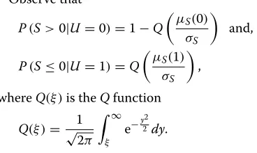
. The BER performance is now obtained as
Observe that
RemarkThe BER for a pure RCM code can be esti-mated as a particular case of the parallel LDGM-RCM withd(LDGMv) =0.
4 Results and discussion
In this section, we evaluate the proposed EXIT chart
analysis and BER prediction method of Section 3 for
both AWGN and fast fading Rayleigh channels. We
begin by considering the AWGN channel. Section 4.1
presents some mutual information trajectories of actual codes on the corresponding EXIT charts. In Section4.2, we compare the BER predictions obtained using these charts with the BER obtained by Monte Carlo
simu-lations. In Section 4.3, the EXIT analysis is used to
obtain codes that approach the Shannon theoretical limit. Finally, the extension to Rayleigh channels is considered in Section4.4.
4.1 Trajectories
We begin in Fig.4by showing the EXIT chart of a pure
RCM code with weight set D = {2, 3, 4, 8} and
spec-tral efficiency ρ = 7.4 for three different SNR values,
0 0.1 0.2 0.3 0.4 0.5 0.6 0.7 0.8
Fig. 4EXIT chart, BER contour lines, and mutual information trajectory for a pure RCM code ofρ=7.4 when transmitting a non-uniform source with entropyH(p0)=0.72 over an AWGN channel
17, 18, and 20.25 dB, and for a non-uniform source with entropy H(p0) = 0.72 (p0 = 0.8). Notice that the vari-able node curve (which is valid for all SNRs) ends at the point(H(p0),H(p0))as it should be. Also plotted in the figure are the Monte Carlo simulated mutual information
trajectories of this code with block length K = 37000
(and M = 10000). Each trajectory is plotted using the
same color as their corresponding SNR’s EXIT chart CN curve, and they end where the corresponding CN and VN curves intersect. In addition, the contour lines of the cor-responding simulated BERs are also shown. For example, at SNR= 17 dB, the BER of the code is 5.5·10−2 and, as observed, the blue curve of the EXIT chart intersects the VN decoder curve very close to the 5.5·10−2 con-tour line. Similarly, for SNR= 18 dB and 20.25 dB, the simulated BERs are 3.3·10−2and 2.2·10−3, respectively. Again, the intersections between CN and VN curves occur very close to the corresponding BER’s contour lines. Note however that none of these SNRs allow the channel to be open.
As previously explained , RCM-LDGM codes substi-tute some RCM symbols with non-systematic LDGM QPSK modulated bits, with the goal to lower the
error floor of the corresponding RCM code. Figure 5
shows the EXIT chart and mutual information trajec-tories for the RCM-LDGM code obtained by substi-tuting 200 RCM symbols by 200 LDGM coded binary
symbols (with d(LDGMv) = 1) in the previous RCM
configuration.
Observe that by introducing these 200 LDGM coded bits, we avoid the previous intersection of the curves at SNR 20.25 dB, improving in this way the BER at 20.25 dB. The corresponding mutual information trajectory at
0 0.1 0.2 0.3 0.4 0.5 0.6 0.7 0.8
SNR 20.25 is shown in Fig.5. Since the channel is open, it reaches its maximal value, i.e., (0.72,0.72). It turns out that SNR = 20.25 is the smallest SNR that allows the channel to remain open, and as such, it is the corresponding decod-ing threshold of the given code. In the same figure, the trajectory at SNR = 19.25 dB is also shown, but in this case the channel is closed and does not reach the maximum value.
4.2 Bit error rate from the EXIT charts
As explained in Section 3.4, an estimated BER can be
assigned to each point of the variable node (VN) curve of the EXIT chart. Therefore, the BER of a particular code at a given SNR is obtained from the value of the VN point where the CN and VN curves intersect.
In this section, we will consider two different
RCM-LDGM configurations withρ = 4 given byK = 25000,
M = 12365, and I = 135, with dLDGM(v) 1 and 2.
Moreover, we will consider three different sources with
p0 = 0.5, p0 = 0.8, and p0 = 0.95 and three
differ-ent weight sets D = {1, 1, 1, 1, 2, 2},{1, 1, 2, 2, 4, 4}, and
{2, 2, 3, 3, 4, 4}. Recall that the VN curve of the EXIT chart depends onM, I, dLDGM(v) , and d(RCMc) , whereas the CND
curve depends also on the actual values of D and on
the SNR.
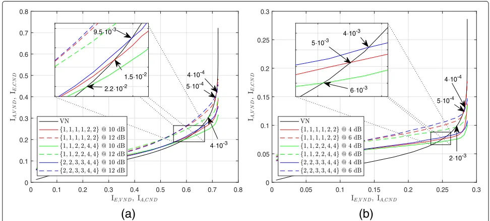
Figure 6a shows the EXIT chart of the configuration
with d(LDGMv) = 1 for the different weight sets and two SNR values, 10 and 12 dB. The plot shows the BER esti-mated values at the intersecting points. For example, for
the configuration described above with{1, 1, 1, 1, 2, 2}, the estimated BERs are 1.5·10−2at SNR=10 dB and 5·10−4 at SNR=12 dB. When{1, 1, 2, 2, 4, 4}, the estimated BERs are 2.2·10−2at SNR=10 dB and 3·10−3at SNR=12 dB. Finally, for{2, 2, 3, 3, 4, 4}, we obtain 9.5·10−3and 4·10−4, respectively. Similarly, Fig.6b shows the EXIT curves at SNR= 4 and 6 dB for the configuration withd(LDGMv) =
2 with their estimated BER values when transmitting a source with p0 = 0.95. SinceH(0.95) = 0.28, the VN curve ends at point (0.28,0.28).
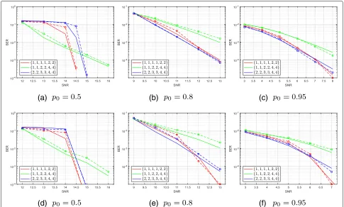
In order to corroborate our BER predictions, Fig.7 com-pares the BER curves obtained by Monte Carlo simulation with those obtained by the EXIT chart BER estimation, as it is done in Fig. 6. As it can be seen in the figure, the predictions are accurate for both uniform and non-uniform sources.
The parameters of these codes have not been optimized, and therefore, they present a large gap to the correspond-ing Shannon limits given by 10·log102ρ·H(S)−1, which
correspond to 0.91, 8.06, and 11.76 dB for p0 = 0.95,
p0 = 0.8, andp0 = 0.5, respectively. In the next section, we will obtain near capacity high spectral efficiency codes using the EXIT chart analysis.
4.3 Code design based on the decoding threshold for AWGN channels
The idea behind the design method is to start with a pool of possible codes having the required rate and then obtain the EXIT charts for the source of interest. The codes with the lower decoding threshold or those whose curves
0 0.1 0.2 0.3 0.4 0.5 0.6 0.7 0.8
0 0.1 0.2 0.3 0.4 0.5 0.6 0.7 0.8
9.5 10-3
2.2 10-2 1.5 10-2
4 10-3 4 10-4
5 10-4
(a)
0 0.05 0.1 0.15 0.2 0.25 0.3
0 0.05 0.1 0.15 0.2 0.25 0.3
6 10-3 5 10-3
4 10-3
2 10-3 4 10-4
5 10-4
(b)
(a)
(b)
(c)
(d)
(e)
(f)
Fig. 7Predicted (dashed line) and Monte Carlo simulated (continuous line) BER vs SNR curves for the RCM-LDGM codes.a–cThe configuration with d(v)LDGM=1.d–fThe configuration withdLDGM(v) =2. An AWGN channel is considered
intersect closer to the maximum point(H(p0),H(p0)are kept. The resulting subset of codes are then tuned-up by slightly changing their designed parameters. We have observed the following trends:
1 For sources with smaller entropy, larger RCM weight sets,D, tend to work better, since the sum-product algorithm is aided by the a priori probability. 2 When designing the LDGM part of the code, there is
a trade-off regarding the numberI of LDGM binary symbols. By increasingI, more residual errors are corrected in the waterfall region, making it steeper. However, larger SNRs are required to reach this waterfall region.
3 The range for parameterd(LDGMv) is between 1 and 5. The larger parameterI is, the larger value ford(LDGMv) can be selected.
Next, we provide EXIT chart design examples for an
RCM-LDGM code with a spectral efficiencyρ = 7.4 for
the transmission over AWGN channels of three memory-less sources with a priori probabilitiesp0=0.5,p0=0.8,
and p0 = 0.95. The corresponding Shannon limits are
at 22.25 dB, 15.97 dB, and 5.24 dB, respectively. Table 1
shows the best codes obtained by the EXIT chart analysis for a code lengthK= 37000 bits.
The corresponding EXIT charts and real trajectories of the designed codes are plotted in Fig.8. Note from Fig.8c that when transmitting the uniform source (p0 = 0.5), the channel between both EXIT curves remains open at
SNR = 24.15 dB (1.9 dB from the Shannon limit) and,
consequently, the received blocks should be decoded with a low probability of error. However, if this same code was used to transmit the symbols generated by the
non-uniform source (p0 = 0.8) by only modifying the a
Table 1Best configurations obtained by the EXIT chart analysis for AWGN channels
p0 K M I d(v)LDGM D Decoding
threshold (dB)
0.5 37000 9800 200 1 {2, 3, 4, 8} 24.15
0.8 37000 9720 280 4 {2, 2, 3, 3, 4, 8} 18.2
0.95 37000 9200 800 3 {1, 1, 1, 1, 1, 1, 7.25
(a)
(b)
(c)
Fig. 8EXIT chart and real trajectories of the designed codes for AWGN channels and sources withcp0=0.5,bp0=0.8, andap0=0.95
priori probability to 0.8 in the SP algorithm, the decod-ing threshold would decrease to 20.15 dB (refer Fig.5). This is still 4 dB away from the Shannon limit. The opti-mized code for this source is given in Table 1. Notice that the gap is reduced to 2.23 dB (refer to Fig.8b). This clearly shows that when transmitting binary symbols gen-erated by a non-uniform source, the channel code behaves like a joint source-channel code and, therefore, it has to be designed according to the source. Finally, Fig.8a plots the EXIT chart of the best found configuration when
transmitting the non-uniform source with p0 = 0.95.
The decoding threshold is only 2.01 dB away from the Shannon limit.
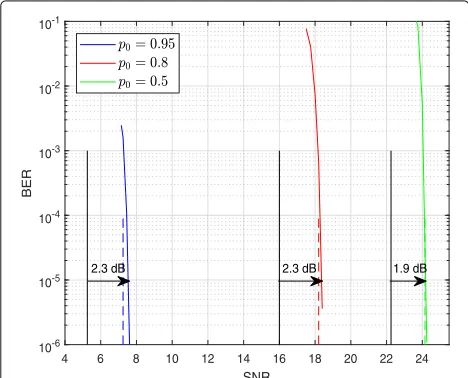
In order to corroborate that the codes obtained from the EXIT chart analysis perform as expected, Fig.9plots
4 6 8 10 12 14 16 18 20 22 24
SNR
10-6
10-5
10-4
10-3
10-2
10-1
BER
1.9 dB 2.3 dB
2.3 dB
Fig. 9BER vs SNR behavior of the obtained codes forp0=0.5,
p0=0.8, andp0=0.95. The Shannon limits (continuous lines) and the predicted decoding threshold (dashed lines) are plotted as vertical lines. An AWGN channel is considered
the BER vs SNR curves obtained by Monte Carlo simula-tions, as well as the theoretical decoding thresholds for the designed codes (shown as vertical dashed lines), and the corresponding Shannon limits (vertical black lines). Note from the Monte Carlo simulations that the code designed forp0 = 0.5 is 1.9 dB away from its Shannon limit for a BER = 10−5, while the codes optimized for the sources withp0=0.8 andp0= 0.95 present both a gap of 2.3 dB with respect to the Shannon limits. The figure indicates that the decoding threshold obtained from the EXIT chart analysis very accurately predicts the waterfall region. For
the source with p0 = 0.5, the gap between the
decod-ing threshold and the waterfall region at BER = 10−5 is not appreciable, whereas for the sources with p0 = 0.8 andp0 = 0.95, these gaps are 0.1 dB and 0.3 dB, respec-tively. An explanation for the gap increase is that for non-uniform sources longer blocks are required to maintain stationarity.
Table2summarizes the simulation time, as well as the computational time of the EXIT chart analysis, required
to obtain the BER vs SNR points of the codeK = 37000,
M= 9800,I = 200,dLDGM(v) = 1, andD= {2, 3, 4, 8}. As shown in the table, the EXIT chart analysis is much faster
Table 2Computational time required to predict a BER vs SNR
point in Fig.9
BER EXIT chart Monte Carlo simulation Reduction factor
Average convergence time per block
Blocks for 10 errors
10−3 10s 229s 1 22.9
10−4 10s 113s 3 33.9
10−5 10s 96s 27 259.2
(a)
(b)
(c)
Fig. 10EXIT chart and real trajectories of the designed codes for fast Rayleigh channel and sources withcp0=0.5,bp0=0.8, andap0=0.95
than the simulations, making the search by trial and error feasible.
4.4 Extension to fast fading Rayleigh channels
We now look at the behavior of the EXIT chart analy-sis when considering fast fading Rayleigh channels. Note that the only modification that has to be introduced in this case is in step 2 of the SP algorithm (see Section3.2). Specifically, since we are assuming perfect channel state information (CSI) at the receiver, the fading factor that multiplies the coded RCM-LDGM symbols (i.e., realiza-tions of i.i.d. exponential random variables) has to be provided to the decoder.
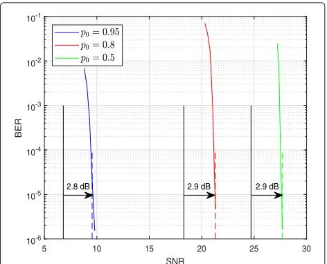
As in the previous AWGN case, we focus on the EXIT chart design for codes of spectral efficiencyρ = 7.4 bits per complex dimension and with sources having a priori probabilities p0 = 0.5, p0 = 0.8, and p0 = 0.95. The corresponding SNR Shannon limits are 24.7 dB, 18.3 dB, and 6.8 dB, respectively. Figure 10 is similar to Fig. 8, except that we now consider fast fading. It plots the EXIT charts and real trajectories of the good codes, specified in Table3, which have been selected by our EXIT chart analysis. The EXIT chart channels are open at SNRs close to the Shannon limits. This is shown in Fig. 11, where the BER predictions and the actual Monte Carlo simula-tions are presented for different values of SNR. Note that the gaps to the Shannon limits are within 3 dB and that
Table 3Best configurations obtained by the EXIT chart analysis for fast fading Rayleigh channels
p0 K M I dLDGM(v) D Decoding
threshold (dB)
0.5 37000 9600 300 3 {2, 3, 4, 4, 8} 27.7
0.8 37000 9240 760 5 {2, 2, 3, 3, 4, 8} 21.3
0.95 37000 9480 520 4 {1, 1, 1, 1, 1, 1, 1, 1, 1, 1, 1, 1} 9.55
the BER predictions are very close to the results obtained by simulations, corroborating that the proposed EXIT chart analysis is also well suited for fast fading Rayleigh channels.
5 Conclusion
Parallel RCM-LDGM codes are very well suited for imple-menting smooth high rate adaptation when transmitting uniform and non-uniform binary memoryless sources. However, when long block lengths are considered, the search of good design parameters using a brute force approach is time consuming. To speed up the design process, we have successfully developed an EXIT chart analysis for these codes, which presents the challenge of the combination of analog and digital check nodes,
5 10 15 20 25 30
SNR
10-6
10-5
10-4
10-3
10-2
10-1
BER
B d 9 . 2 B
d 9 . 2 B
d 8 . 2
something not encountered in other works. By assum-ing a linear relationship between the variances of the LLR messages in both types of CNs, very precise EXIT charts are obtained for the case of AWGN and fast fading Rayleigh channels. The predicted BER vs SNR curves are very close to the results obtained through simulations.
Endnotes
1Without loss of generality, it is assumed thatK is an
even integer.
2A multiset is a generalization of the concept of a set
that, unlike a set, allows multiple instances of the multi-set’s elements.
3The a priori probability of the source symbols is
already considered in step 1 of the SPA.
Appendix Obtainingκ
The constantκ is computed by Monte Carlo simulation
through the following iterative procedure:
1 Start with an initial value ofκin (12) (sayκ =1), and choose a value forσR2,Aso that the corresponding value of the mutual information computed by the PDF in (11) is in the range (0.5,0.9). For the value of σ2
R,Aunder consideration, generate the extrinsic
messages passed from the VN to the RCM and LDGM check nodes according to (14) and (15), respectively. 2 Run one iteration of the sum-product algorithm to
obtain the extrinsic LLR messages passed from each LDGM and RCM check nodes to the VN, and obtain their empirical conditional PDFs.
3 Defineκ1as the ratio between the variances of the empirical conditional distributions of RCM and LDGM check nodes obtained in step 2.
4 Repeat the previous 3 steps, usingκ1as the initial value forκ, until the value ofκ1in step 3 is close enough to the value ofκ1in the previous iteration. 5 Setκ =κ1in the distribution (12).
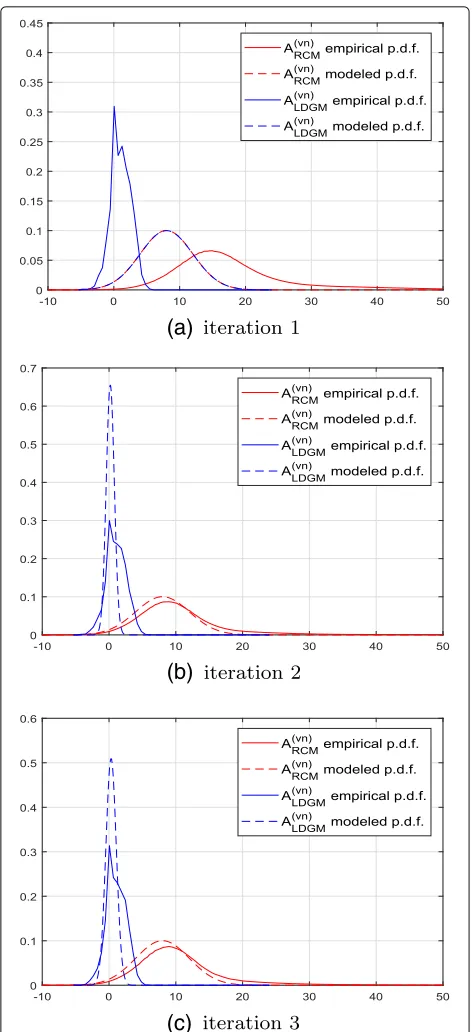
Figure12shows a graphical example of the steps fol-lowed to find κ. The initial empirical conditional PDFs (i.e., when κ = 1) are shown in Fig. 12a. As it can be observed, none of the LLR messages is appropriately mod-eled at this point, since the initial value forκ(κ = 1) was chosen arbitrarily. Note that sinceκ = 1, the modeled
A(RCMVN)is equal toA(LDGMVN) . The value ofκ obtained in step 3 is 43, and the corresponding empirical conditional dis-tributions are shown in the Fig.12b. Notice that for this value ofκ, the messages are better modeled by (11) and (12). However, the process is not finished yet. The second iteration results inκ = 26. The corresponding empirical conditional distributions are shown in the Fig.12c. If we
(a)
(b)
(c)
Fig. 12Example of the iterative procedure to findκfor the EXIT chart of Fig.8c. The histograms (conditioned toU=1) obtained by Monte Carlo simulations are plotted in blue and the corresponding modeled conditional PDFs in red (refer to (11) and (12)).aIteration 1.bIteration 2.
cIteration 3
Abbreviations
ACM: Adaptive coded modulation; APSK: Amplitude and phase-shift keying; AWGN: Additive white Gaussian noise; BER: Bit error rate; BICM:Bit-interleaved coded modulation; CN(D): Check node (decoder); EXIT: Extrinsic information transfer; LDGM: Low-density generator matrix; LDPC: Low-density parity check; LLR: Log-likelihood ratio; PDF: Probability density function; QAM: Quadrature amplitude modulation; RCM: Rate compatible modulation; RV: Random variable; SNR: Signal to noise ratio; SP(A): Sum-product (algorithm); VN(D): Variable node (decoder)
Funding
This work was supported in part by the Spanish Ministry of Economy and Competitiveness through the CARMEN project (TEC2016-75067-C4-3-R), the COMONSENS network (TEC2015-69648-REDC) and by NSF Award CCF-1618653.
Availability of data and materials
Data sharing is not applicable to this article as no datasets were generated or analysed during the current study.
Authors’ contributions
JG-F and PMC conceived the research question. IG and PMC proved the main results. IG, PMC, and JG-F wrote the paper. All authors have read and approved the final manuscript.
Competing interests
The authors declare that they have no competing interests.
Publisher’s Note
Springer Nature remains neutral with regard to jurisdictional claims in published maps and institutional affiliations.
Author details
1Department of Basic Science, University of Navarra, Mikeletegi Pasealekua, 48,
20018 San Sebastian, Spain.2Department of Electrical and Computer
Engineering, University of Delaware, 307 Evans Hall, 19716 Newark, USA.
Received: 30 July 2018 Accepted: 14 December 2018
References
1. H. Cui, C. Luo, J. Wu, C. W. Chen, F. Wu, Compressive coded modulation for seamless rate adaptation. IEEE Trans. Wirel. Commun.12(10), 4892–4904 (2013)
2. H. Cui, C. Luo, K. Tan, F. Wu, C. W. Chen, inProceedings of the 14th ACM International Conference on Modeling, Analysis and Simulation of Wireless and Mobile Systems. Seamless rate, adaptation for wireless networking (ACM, New York, 2011), pp. 437–446.http://doi.acm.org/10.1145/ 2068897.2068971.
3. W. Zhong, J. Garcia-Frias, LDGM codes for channel coding and joint source-channel coding of correlated sources. EURASIP J. Appl. Sig. Process.2005, 942–953 (2005)
4. W. Zhong, H. Chai, J. Garcia-Frias, inInformation Theory, 2005. ISIT 2005. Proceedings. International Symposium On. Approaching the Shannon limit through parallel concatenation of regular LDGM codes (IEEE, 2005), pp. 1753–1757.https://doi.org/10.1109/ISIT.2005.1523646
5. J. M. Kroll, N. Phamdo, Source-channel optimized trellis codes for bitonal image transmission over AWGN channels. IEEE Trans. Image Process.8(7), 899–912 (1999)
6. P. Burlina, F. Alajaji, An error resilient scheme for image transmission over noisy channels with memory. IEEE Trans. Image Process.7(4), 593–600 (1998)
7. G.-C. Zhu, F. Alajaji, Turbo codes for nonuniform memoryless sources over noisy channels. IEEE Commun. Lett.6(2), 64–66 (2002)
8. G.-C. Zhu, F. Alajaji, J. Bajcsy, P. Mitran, Transmission of nonuniform memoryless sources via nonsystematic turbo codes. IEEE Trans. Commun. 52(8), 1344–1354 (2004)
9. J. Hagenauer, Source-controlled channel decoding. IEEE Trans. Commun. 43(9), 2449–2457 (1995)
10. L. Li, J. Garcia-Frias, inInformation Sciences and Systems (CISS), 2014 48th Annual Conference On. Hybrid analog-digital coding scheme based on parallel concatenation of linear random projections and LDGM codes (IEEE, 2014), pp. 1–6.https://doi.org/10.1109/CISS.2014.6814118
11. L. Li, J. Garcia-Frias, inInformation Sciences and Systems (CISS), 2015 49th Annual Conference On. Hybrid analog-digital coding for nonuniform memoryless sources (IEEE, 2015), pp. 1–5.https://doi.org/10.1109/CISS. 2015.7086861
12. G. Caire, G. Taricco, E. Biglieri, Bit-interleaved coded modulation. IEEE Trans. Inf. Theory.44(3), 927–946 (1998)
13. F. Cabarcas, R. D. Souza, J. Garcia-Frias, Turbo coding of strongly nonuniform memoryless sources with unequal energy allocation and PAM signaling. IEEE Trans. Sig. Process.54(5), 1942–1946 (2006) 14. I. Ochoa, P. M. Crespo, M. Hernaez, LDPC codes for non-uniform
memoryless sources and unequal energy allocation. IEEE Commun. Lett. 14(9), 794–796 (2010)
15. S. Ten Brink, Convergence behavior of iteratively decoded parallel concatenated codes. IEEE Trans. Commun.49(10), 1727–1737 (2001) 16. S. Ten Brink, G. Kramer, A. Ashikhmin, Design of low-density parity-check
codes for modulation and detection. IEEE Trans. Commun.52(4), 670–678 (2004)
17. J. Wu, Z. Teng, H. Cui, C. Luo, C. xHuang, H.-H. Chen, Arithmetic-BICM for seamless rate adaptation for wireless communication systems. IEEE Syst. J. 10(1), 228–239 (2016)
18. J. Du, L. Yang, J. Yuan, L. Zhou, X. He, Bit mapping design for LDPC coded BICM schemes with multi-edge type exit chart. IEEE Commun. Lett.21(4), 722–725 (2017)
19. T. Cheng, K. Peng, J. Song, K. Yan, EXIT-aided bit mapping design for LDPC coded modulation with APSK constellations. IEEE Commun. Lett.16(6), 777–780 (2012)
20. D. J. MacKay, Good error-correcting codes based on very sparse matrices. IEEE Trans. Inf. Theory.45(2), 399–431 (1999)