R E V I E W
Open Access
Robust distributed cooperative RSS-based
localization for directed graphs in mixed
LoS/NLoS environments
Luca Carlino
1, Di Jin
2*, Michael Muma
2and Abdelhak M. Zoubir
2Abstract
The accurate and low-cost localization of sensors using a wireless sensor network is critically required in a wide range of today’s applications. We propose a novel, robust maximum likelihood-type method for distributed cooperative received signal strength-based localization in wireless sensor networks. To cope with mixed LoS/NLoS conditions, we model the measurements using a two-component Gaussian mixture model. The relevant channel parameters, including the reference path loss, the path loss exponent, and the variance of the measurement error, for both LoS and NLoS conditions, are assumed to be unknown deterministic parameters and are adaptively estimated. Unlike existing algorithms, the proposed method naturally takes into account the (possible) asymmetry of links between nodes. The proposed approach has a communication overhead upper-bounded by a quadratic function of the number of nodes and computational complexity scaling linearly with it. The convergence of the proposed method is guaranteed for compatible network graphs, and compatibility can be tested a priori by restating the problem as a graph coloring problem. Simulation results, carried out in comparison to a centralized benchmark algorithm, demonstrate the good overall performance and high robustness in mixed LoS/NLoS environments.
Keywords: Cooperative localization, Received signal strength (RSS), Maximum likelihood estimation, Wireless sensor network (WSN)
1 Introduction
The wide spread of telecommunication systems has led to the pervasiveness of radiofrequency (RF) signals in almost every environment of daily life. Knowledge of the location of mobile devices is required or beneficial in many appli-cations [1], and numerous localization techniques have been proposed over the years [1–4]. Techniques based on the received signal strength (RSS) are the preferred option when low cost, simplicity, and technology obliviousness are the main requirements. In some standards, e.g., IEEE 802.15.4, an RSS indicator (RSSI) is encoded directly into the protocol stack [5]. In addition, RSS is readily avail-able from any radio interface through a simple energy detector and can be modeled by the well-known path loss model [6] regardless of the particular communication
*Correspondence:[email protected]
2Signal Processing Group, Department of Electrical Engineering and Information Technology, Technische Universität Darmstadt, Darmstadt, Germany
Full list of author information is available at the end of the article
scheme. Based on that, RSS can be exploited to implement “opportunistic” localization for different wireless tech-nologies, e.g., Wi-Fi [7], FM radio [8], or cellular networks [9]. In the context of wireless sensor networks (WSNs), nodes with known positions (anchors) can be used to localize the nodes with unknown positions (agents). Gen-erally speaking, localization algorithms can be classified according to three important categories.
Centralized vs. distributed.Centralized algorithms, e.g., [10–14], require a data fusion center that carries out the computation after collecting information from the nodes, while distributed algorithms, such as [15,16], rely on self-localization and the computation is spread throughout the network. Centralized algorithms are likely to provide more accurate estimates, but they suffer from scalabil-ity problems, especially for large-scale WSNs, while dis-tributed algorithms have the advantage of being scalable and more robust to node failures [17].
Cooperative vs. non-cooperative. In a non-cooperative algorithm, e.g., [18], each agent receives information only
from anchors. For all agents to obtain sufficient informa-tion to perform localizainforma-tion, non-cooperative algorithms necessitate either long range (and high-power) anchor transmission or a high-density of anchors [17]. In cooper-ative algorithms, such as [19,20], inter-agent communica-tion removes the need for all agents to be in range of one (or more) anchors [17].
Bayesian vs. non-Bayesian.In non-Bayesian algorithms, e.g., expectation-maximization (EM) [21], and its variant, expectation-conditional maximization (ECM) [22], the unknown positions are treated as deterministic, while in Bayesian algorithms, e.g., nonparametric belief propaga-tion (NBP) [23] and sum-product algorithm over wireless networks (SPAWN) [24,25] and its variant Sigma-Point SPAWN [26], the unknown positions are assumed to be random variables with a known prior distribution.
Many existing works on localization using RSS mea-sures, such as [27] and [28], are based on the assump-tion that the classical path loss propagaassump-tion model is perfectly known, mostly via a calibration process. How-ever, this assumption is impractical for two reasons. Firstly, conducting the calibration process requires inten-sive human assistance, which may be not affordable, or may even be impossible in some inaccessible areas. Secondly, the channel characteristics vary due to mul-tipath (fading), and non-negligible modifications occur also due to mid- to long-term changes in the environ-ment, leading to non-stationary channel parameters [29]. This implies that the calibration must be performed continuously [29, 30] because otherwise the resulting mismatch between design assumptions and actual oper-ating conditions leads to severe performance degra-dation. These facts highlight the need for algorithms that adaptively estimate the environment and the loca-tions. A further difficulty is due to the existence of non-line-of-sight (NLoS) propagation in practical local-ization environments. Among various works handling the NLoS effect, a majority of them have treated the NLoS meaures as outliers and tried to neglect or mit-igate their effect, including the maximum likelihood (ML)-based approach [31,32], the weighted least-squares (WLS) estimator [32, 33], the constrained localiza-tion techniques [34, 35], robust estimators [36, 37], and the method based on virtual stations [38]. In contrast to these works, several approaches, includ-ing [21, 22, 39], have proposed specific probabilistic models for the NLoS measures, therewith exploit-ing the NLoS measures for the localization purpose. In the light of these considerations, our aim is to develop an RSS-based, cooperative localization frame-work that frame-works in mixed LoS/NLoS environments, requires no knowledge on parameters of the propa-gation model, and can be realized in a distributed manner.
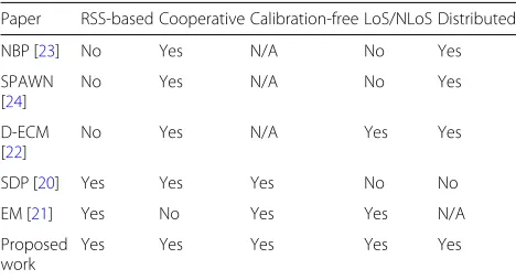
The following distinction is made: only algorithms that directly use RSS measures as inputs are considered RSS-based in the strict sense, while algorithms such as NBP [23], SPAWN [24], distributed-ECM (D-ECM) [22], and their variants are here calledpseudo-RSS-based, because they use range estimates as inputs. Generally speaking, among these two options, RSS-based location estimators are preferred for the following reasons. Firstly, infer-ring the range estimates from the RSS measures usually requires knowledge on the (estimated) propagation model parameters. The assumption of a priori known parame-ters violates the calibration-free requirement. Secondly, even with perfectly known model parameters, there exists no efficient estimator for estimating the ranges from the RSS measures, as proven in [40]. Thirdly, dropping the idealistic assumption of known channel parameters and using their estimates introduce an irremovable large bias, as demonstrated in [41]. Based on these considerations, pseudo-RSS-based approaches do not meet the require-ments in this work. Furthermore, Bayesian approaches, including NBP [23] and SPAWN [24,25], do not consider mixed LoS/NLoS environments. As one representative RSS-based cooperative localization algorithm, Tomic et al.’s semidefinite-programming (SDP) estimator in [20] requires no knowledge on the propagation model, but it does not apply to and cannot be readily extended to a mixed LoS/NLoS environment. To the best of our knowl-edge, the existing works on RSS-based calibration-free localization in a mixed LoS/NLoS environment is rather limited. Yin et al. have proposed an EM-based estimator in [21], but only for the single-agent case. In this paper, we consider a multi-agent case and aim to develop a location estimator that is RSS-based, cooperative, and calibration-free and works in a mixed LoS/NLoS environment. To capture the mixed LoS/NLoS propagation conditions, we adopt the mode-dependent propagation model in [21]. The key difference between this work and [21] lies in whether the localization environment is cooperative or not. More precisely, [21] is concerned with the conven-tional single-agent localization while this work studies cooperative localization in case of multi-agent. Further-more, we develop a distributed algorithm, where model parameters and positions are updated locally by treating the estimated agents as anchors, inspired by the works in [42–44]. A succinct characterization of the proposed work and its related works is listed in Table1.
Table 1Succinct characterization of the related works and the proposed work
Paper RSS-based Cooperative Calibration-free LoS/NLoS Distributed
NBP [23] No Yes N/A No Yes
Yes Yes Yes Yes Yes
N/Anot applicable. The terms “RSS-based,” “Cooperative,” “Calibration-free,” “LoS/NLoS,” and “Distributed” are defined and discussed in Section1
of coping with mixed LoS/NLoS conditions. Simulation results, carried out in comparison with a centralized ML algorithm that serves as a benchmark, show that the pro-posed approach has good overall performance. Moreover, it adaptively estimates the channel parameters, has accept-able communication overhead and computation costs, thus satisfying the major requirements of a practically viable localization algorithm. The convergence analysis of the proposed algorithm is conducted by restating the problem as a graph coloring problem. In particular, we formulate a graph compatibility test and show that for compatible network structures, the convergence is guar-anteed. Unlike existing algorithms, the proposed method naturally takes into account the (possible) asymmetry of links between nodes.
The paper is organized as follows. Section 2 formu-lates the problem and details the algorithms. Section 3
discusses convergence. Section 4 presents the simula-tions results, while Section5concludes the paper. Finally, AppendicesAandBcontain some analytical derivations which would otherwise burden the reading of the paper.
2 Methods/experimental
2.1 Problem formulation
Consider1 a directed graph with Na anchor nodes and
Nu agent nodes, for a total of N = Na + Nu nodes.
In a two-dimensional (2D) scenario, we denote the posi-tion of nodeiby xi =[xi yi]∈ R2×1, wheredenotes
transpose. Between two distinct nodesiandj, the binary variableoj→iindicates if a measure, onto directionj→i,
is observed (oj→i = 1) or not (oj→i = 0). In the case
wheni = j, since a node does not self-measure, we have oi→i =0. This allows us to define the observation matrix
O∈BN×N with elementso
i,joi→jas above. The
afore-mentioned directed graph has connection matrix O. It is important to remark that, for a directed graph,O is not necessarily symmetric; physically, this models possible
channel anisotropies, miss-detections and, more gener-ally, link failures. Let mj→i be a binary variable, which
denotes if the link j → i is LoS (mj→i = 1) or NLoS
(mj→i = 0). Due to physical reasons,mj→i = mi→j. We
define the LoS/NLoS matrix2L∈BN×Nof elementsli,j
mi→j, and we observe that, sincemj→i=mi→j, the matrix
is symmetric, i.e.,L = L. We stress that this symmetry is preserved regardless ofO, as it derives from physical reasons only. Let(i)be the(open) neighborhoodof node i, i.e., the set of all nodes from which node i receives observables (RSS measures), formally:(i) {j = i : oj→i=1}. We definea(i)as the anchor-neighborhood of
nodei, i.e., the subset of(i)which contains only anchor nodes as neighbors of node i. We also define u(i) as
the agent-neighborhood of nodei, i.e., the subset of(i) which contains only agent nodes as neighbors of nodei. In general,(i)=a(i)∪u(i).
2.2 Data model
In the sequel, we will assume that all nodes are stationary and that the observation time-window is sufficiently short in order to neglect correlation in the shadowing terms. In practice, such a model simplification allows for a more analytical treatment of the localization problem and has also been used, for example, in [11,12]. Following the path loss model and the data models present in the literature [17, 21] and denoting by K the number of samples col-lected on each link over a predetermined time window, we model the received power at time indexkfor anchor-agent links as
while, for the agent-agent link,
ru(m→)i(k)=
• p0LOS/NLOSis the reference power (in dBm) for the LoS
• αLOS/NLOSis the path loss exponent for the LoS or
NLoS case;
• xais the known position of anchora;
• xuis the unknown position of agentu (similarly for
xi);
• a(i),u(i)are the anchor- and
agent-neighborhoods of nodei, respectively; • The noise termswa→i(k),va→i(k),wu→i(k),and
vu→i(k)are modeled as serially independent and
identically distributed (i.i.d.), zero-mean, Gaussian random variables, independent from each other (see below), with variances:
Var[wa→i(k)]=Var[wu→i(k)]=σLOS2 ,
Var[va→i(k)]=Var[vu→i(k)]=σNLOS2 ,
andσNLOS2 > σLOS2 >0.
More precisely, letting δi,j be Kronecker’s delta3, the
independence assumption is formalized by the following equations
ous equations imply that two different links are always independent, regardless of the considered time instant. In this paper, we call this property link independence. If only one link is considered, i.e., j2 = j1 and i2 =
i1, then independence is preserved by choosing
differ-ent time instants, implying that the sequencewj→i k
wj→i(1),wj→i(2),. . . is white. The same reasoning
applies to the (similarly defined) sequence {vj→i}k. As
a matter of notation, we denote the unknown posi-tions (indexing the agents before the anchors) by x
It is important to stress that, in a more realistic sce-nario, channel parameters may vary from link to link and also across time. However, such a generalization would produce an under-determined system of equations, thus giving up uniqueness of the solution and, more generally, analytical tractability of the problem. For the purposes of this paper, the observation model above is sufficiently gen-eral to solve the localization task while retaining analytical tractability.
2.3 Time-averaged RSS measures
Motivated by a result given in AppendixA, we consider the time-averaged RSS measures, defined as
¯
as our new observables4. While it would have been prefer-able to work with the original data from a theoretical standpoint, several considerations lead to the preference of time-averaged data, most notably: (1) comparison with other algorithms present in the literature, where the data model assumes only one sample per link, i.e., K = 1, which is simply a special case in this paper; (2) reduced computational complexity in the subsequent algorithms; (3) if the RSS measures onto a given link needs to be com-municated between two nodes, the communication cost is notably reduced, since only one scalar, instead ofK sam-ples, needs to be communicated; (4) formal simplicity of the subsequent equations.
Moreover, from AppendixA, it follows that, assuming known L, the ML estimators of the unknown positions based upon an original data or a time-averaged data are actually the same. To see this, it suffices to choose θ =(x,p0LOS,p0NLOS,αLOS,αNLOS)and
for j ∈ (i) and splitting the additive noise term as required. For a fixed link, only one of two cases (LoS or NLoS) is verified, thus applying (34) of AppendixAyields
arg max
We define Ri as the set of all RSS measures that
node i receives from anchor neighbors, i.e., Ri
ra(m→)i(1),. . .,ra(m→)i(K):a∈a(i)
,Zias the set of all RSS
measures that nodeireceives from agent neighbors, i.e., Zi
r(j→m)i(1),. . .,r(j→m)i(K):j∈u(i)
, andYi as the set
of all RSS measures locally available to nodei, i.e.,Yi
Ri ∪Zi. Analogously, for time-averaged measures, we
which represents the information available to the whole network.
2.4 Single-agent robust maximum likelihood (ML)
We first consider the single-agent case, which we will later use as a building block in the multi-agent case. The key idea is that instead of separately treating the LoS and NLoS cases, e.g., by hypothesis testing, we resort to a two-component Gaussian mixture model for the time-averaged RSS measures. More precisely, we assume that the probability density function (pdf ), p(·), of the time-averaged RSS measures, for anchor-agent links, is given by
p(r¯a→i)
Empirically, we can intuitively interpretλi as the
frac-tion of anchor-agent links in LoS (for nodei), whileζias
the fraction of agent-agent links in LoS (for node i). As in [21], the Markov chain induced by our model is regu-lar and time-homogeneous. From this, it follows that the Markov chain will converge to a two-component Gaussian mixture, giving a theoretical justification to the proposed approach.
Assume that there is a single agent, say nodei, with a minimum of three anchors5in its neighborhood (|a(i)| ≥
3), in a mixed LoS/NLoS scenario. Our goal is to obtain the maximum likelihood estimator (MLE) of the position of node i. Let r¯i =
¯
r1→i · · · ¯r|a(i)|→i
∈ R|a(i)|×1
be the collection of all the time-averaged RSS measures available to nodei. Using the previous assumptions and
the independency between the links, the joint likelihood function6p(¯ri;θ)is given by
where the maximization is subject to several constraints:
λi∈(0, 1),αLOS>0,αNLOS>0,σLOS2 >0, andσNLOS2 >0.
In general, the previous maximization admits no closed-form solution, so we must resort to numerical procedures.
2.5 Multi-agent robust ML-based scheme
In principle, our goal would be to have a ML estimate of all theNu unknown positions, denoted byx. Letλ
be the collections of the mixing coefficients. Definingθ =(x,λ,ζ,η), the ML joint estimator
ˆ
θML =arg max
θ p(ϒ;θ) (13)
is, in general, computationally unfeasible and naturally centralized. In order to obtain a practical algorithm, we now resort to a sub-optimal but computationally feasi-ble and distributed approach. The intuition is as follows. Assume, for a moment, that a specific nodeiknowsη,λ, ζand also all the true positions of its neighbors (which we denote byXi). Then, the ML joint estimation problem is
notably reduced, in fact, ˆ
xiML =arg maxx i
p(ϒ;xi) (14)
We now make the sub-optimal approximation of avoid-ing non-local information in order to obtain a distributed algorithm, thus resorting to
where the marginal likelihoods are Gaussian-mixtures and we underline the (formal and conceptual) separa-tion between anchor-agent links and agent-agent links. By taking the natural logarithm, we have
lnpY¯i;xi,Xi,λi,ζi,η
The maximization problem in (15) then reads
ˆ
We can now relax the initial assumptions: instead of assuming known neighbors positionsXi, we will
substi-tute them with their estimates, Xˆi. Moreover, since the
robust ML-based self-calibration can be done without knowing the channel parametersη, we also maximize over them. Lastly, we maximize with respect to the mixing coefficientsλi,ζi. Thus, our final approach is
which estimated positions exist. We can iteratively con-struct (and update) the setˆu(i), in order to obtain a fully
distributed algorithm, as summarized in Algorithm 1. A few remarks are now in order. First, this algorithm imposes some restrictions on the arbitrariness of the net-work topology, since the information spreads starting from the agents which were able to self-localize dur-ing initialization; in practice, this requires the network to be sufficiently connected. Second, convergence of the algorithm is actually a matter of compatibility: if the net-work is sufficiently connected (compatible), convergence is guaranteed. Given a directed graph, compatibility can be tested a priori and necessary and sufficient conditions can be found (see Section 4). Third, unlike many algo-rithms present in the literature, symmetrical links are not necessary, nor do we resort to symmetrization (like NBP): this algorithm naturally takes into account the (possible) asymmetrical links of directed graphs.
Algorithm 1 Robust distributed maximum likelihood (RDML)
Initialization:
Self-Localization: Every node iwith |a(i)| ≥ 3
self-localizes by the robust procedure (12);
Broadcast:Every node which self-localized broadcasts its position estimatexˆi;
Iterative scheme: Start withn←1;
Update position: Every node with|a(i)| + | ˆu(n)(i)| ≥3
estimates its own position by solving (19);
Broadcast:The updated positionxˆ(in)is broadcasted; Update Neighbors:Every nodejfor which the new esti-mated positions xˆ(in) are neighbors updates its own
ˆ
(n)
u (j)with the new positions;
Repeat:Setn ← n+1 and repeat the previous steps until stop condition is met.
Stop condition: | ˆ(n)
u (i)| = |u(i)|for every nodei.
2.6 Distributed maximum likelihood (DML)
As a natural competitor of the proposed RDML algo-rithm, we derive here the distributed maximum likelihood (DML) algorithm, which assumes that all links are of the same type. As its name suggests, this is the non-robust version of the previously derived RDML. As usual, we start with the single-agent case as a building block for the multi-agent case. Using the assumption that all links are the same and the i.i.d. hypothesis, the joint pdf of the time-averaged RSS measures, received by agenti, is given by
We can now proceed by estimating, with the ML crite-rion, firstp0as a function of the remaining parameters,
followed byαas a function ofxiand finallyxi. We have
which is a least-squares (LS) problem and its solution is
By using this expression, the problem of estimatingαas a function ofxiis P⊥A is the orthogonal projection matrix onto the orthog-onal complement of the space spanned by the columns of A. It can be computed via P⊥A = Im − PA, where
PA = A
AA−1Ais an orthogonal projection matrix andIm is the identity matrix of orderm. The solution to
problem (24) is given by
previous expression, we can finally write
ˆ
which, in general, does not admit a closed-form solution, but can be solved numerically. After obtainingxˆi, nodei
can estimatep0andαusing (23) and (25).
The multi-agent case follows an almost identical reason-ing of the RDML. Approximatreason-ing the true (centralized) MLE by avoiding non-local information and assuming to already have an initial estimate ofp0andα, it is possible
to arrive at
where (again) an initialization phase is required and the set of estimated agents-neighborsˆu(i) is iteratively
updated. The key difference with RDML is that, due to the assumption of the links being all of the same type, the estimates of p0 andα are broadcasted and a
com-mon consensus is reached by averaging. This increases the communication overhead, but lowers the computational complexity, operating a trade-off. The DML algorithm is summarized in Algorithm 2.
Similar remarks as for the RDML can be made for the DML. Again, the network’s topology cannot be completely arbitrary, as the information must spread throughout the network starting from the agents which self-localized,
Algorithm 2Distributed maximum likelihood (DML)
Initialization:
Broadcast:Every node which self-localized broadcasts its local estimates
Consensus: All the nodes agree on global values of
(pˆ0,α)ˆ by averaging all the local estimates
Iterative scheme: Start withn←1;
Update position: Every nodeiwitha(i)| + | ˆu(n)(i)≥
3 estimates its own position by solving (27);
Broadcast:The updated positionxˆ(in)is broadcasted; Update Neighbors:Every nodejfor which the new esti-mated positions xˆ(in) are neighbors updates its own
ˆ
(n)
u (j)with the new positions;
Repeat:Setn ← n+1 and repeat the previous steps until stop condition is met.
Stop condition:
ˆ(n)
u (i)= |u(i)|for every nodei.
implying that the graph must be sufficiently connected. Necessary and sufficient conditions to answer the com-patibility question are the same as RDML. Secondly, the (strong) hypothesis behind the DML derivation (i.e., all links of the same type) allows for a more analytical deriva-tion, up to position estimaderiva-tion, which is a nonlinear least-squares problem. However, it is also its weakness since, as will be shown later, it is not a good choice for mixed LoS/NLoS scenarios.
2.7 Centralized MLE with known nuisance parameters (C-MLE)
The centralized MLE ofx with known nuisance param-eters, i.e., assuming knownLandη, is chosen here as a benchmark for both RDML and DML. In the following, this algorithm will be denoted by C-MLE. Its derivation is simple (see AppendixB) and results in
ˆ
are either LoS or NLoS depend-ing on the considered link. It is important to observe that, if all links are of the same type, the dependence from
σ2
j→i in (28) disappears. From standard ML theory [45],
it requires a minimization in a 2Nu-dimensional space, but
still feasible for small values ofNu.
3 Convergence analysis
The convergence test of our proposed algorithm (and also of DML) can be restated as a graph coloring problem: if all the graph can be colored, then it is compatible and convergence is guaranteed. As it is common in the litera-ture on graph theory, letG=(V,E)be a directed graph, withV denoting the set ofnodesandEthe set ofdirected edges. The set of nodes is such thatV = Va∪Vu, where
Vais the (non-empty) set of anchor nodes andVuis the
(non-empty) set of agent nodes.
Definition 1(RDML-initializable)A directed graph G is said to be RDML-initializable if and only if there exists at least one agent node, say x, such that|a(x)| ≥3.
As can be easily checked, the previous statement is a necessary condition: if a graph is not RDML-initializable, then it is incompatible with RDML. To give a neces-sary and sufficient condition, we introduce the notion of “color.” A node can be either black or white; all anchors are black and all agent nodes start as white, but may become black if some condition is satisfied. The RDML can be rewritten as a graph coloring problem. In order to do this, we define the set ˆu(i) {j ∈ u(i) : agentjis black},
i.e., the subset of agent neighbors of nodeiwhich contains only black agent nodes. In general,ˆu(i)⊆u(i). We also
define the set Bu {i ∈ Vu : agentiis black}, i.e., the
set of black agents. In general,Bu ⊆Vu. Given a graphG,
we can perform a preliminary test by running the follow-ing RDML-colorfollow-ing algorithm (a better test will be derived later):
• Initialization(k=0)
1 All anchors are colored black and all agents white; 2 Every agenti with|a(i)| ≥3is colored black;
• Iterative coloring: Start withk=1
1 Every agent witha(i)| + | ˆu(k−1)(i)≥3, where ˆ
(k)
u (i)is the setˆu(i)at stepk, is colored black;
2 Every agentj updates is ownˆ(uk)(j)with the new
colored nodes;
3 The setB(uk)is updated, whereB(uk)is the setBuat
stepk ;
4 Setk←k+1and repeat the previous steps until Vucontains only black nodes.
Suppose that the previous algorithm can color the entire graph black in a finite amount of steps, sayn. Then,nis called RDML-lifetime.
Definition 2 (RDML-lifetime)A directed graph G is said to have RDML-lifetime equal to n if and only if the RDML-coloring algorithm colors black the set Vuin exactly
n steps. If no such integer exists, by convention, n= +∞.
This allows us to formally define compatibility:
Definition 3(RDML-compatibility) A directed graph G is said to be RDML-compatible if and only if:
1 G is RDML-initializable; 2 the RDML-lifetime of G is finite.
Otherwise, G is said to be RDML-incompatible.
In practice, there are only two ways for which a graph is RDML-incompatible: eitherGcannot be initialized, or the RDML-lifetime ofGis infinite. Testing the first condition is trivial; the interesting result is that testing the second condition is made simple thanks to the following.
Theorem 1An initializable graph G is RDML-incompatible if and only if there exist an integer h such that
B(uh)=B(uh−1) ∧ B(uh)<|Vu| (29)
that is, if there is a step h in which no more agents can be colored black and at least one agent is still left white.
Proof (⇐)First, observe that, by construction,
B(uk−1) ⊆B(uk), as black nodes can only be added. LetCG :
N→Nbe the following function
CG(k)=B(uk). (30)
SinceB(uk−1) ⊆ B(uk),CGis non-decreasing. An
RDML-initializable graph is RDML-compatible if and only if it has finite RDML-lifetime, i.e., there must existnsuch that CG(n)= |Vu|. But condition (29) implies that there exists
hsuch thatCG(h) = CG(h−1) < |Vu|. At steph+1
and all successive steps,CGcannot increase since the set
B(uk) cannot change. To show this, the key observation is
that, as the graphGat steph−1 did not satisfy the condi-tions forB(uh−1)to grow (by hypothesis), the set was equal
to itself at step h, i.e.,B(uh−1) = B(uh). But since no color
change happened in Vu at step h, the graphGstill does
not satisfy the conditions forB(uk)to grow fork≥h. Thus,
CG(k) becomes a constant function fork ≥ hand can
never reach the value|Vu|.
(⇒) Since G is an RDML-incompatible graph by hypothesis, at least one agent must be white, soB(uh) < |Vu| is true for anyh. Since CG(k) is non-decreasing, it
sinceB(uk−1) ⊆ B(uk) by construction, B(uh) = B(uh−1) for
someh.
Definition 4(RDML-depth)Let G be a directed graph. Then,
hGinf h
h∈N:B(uh)=B(uh+1) (31)
is called the RDML-depth of G.
A complete graph hashG = 0, as all agents are
col-ored black during the initialization phase of the RDML-coloring algorithm.
Corollary 1Let G be a directed graph. Then, hG ≤ n,
where n is the RDML-lifetime of G.
ProofIfGis not RDML-initializable,hG=0 asB(u0)= ∅.
IfGis RDML-initializable, there are two cases: eithernis finite or not. In the latter,n = +∞andhG is finite by
previous theorem. Ifnis finite,hG=nsinceB(un)= |Vu|
by definition of RDML-lifetime.
The previous corollary proves thathG is always finite,
regardless ofG. This allows us to write the graph com-patibility test, shown in Algorithm 3. Thanks to the pre-vious results, this algorithm always converges and can be used to test a priori if a graph is RDML-compatible or not.
Remark Algorithm 3 can be intuitively explained via a physical metaphor, where, in a metal grid (represent-ing the graph), “heat” (information) spreads out start(represent-ing from some initial “hot spots” (nodes that are colored black in the first iteration). This spreading is continued, reach-ing more and more locations on the grid, until the event occurs that further spreading of “heat” does not change the “heat map.” If, at this point, there are cold spots (nodes that have not been colored black), the graph is RDML-incompatible. By contrast, if heat spreads throughout the grid, the graph is RDML-initializable.
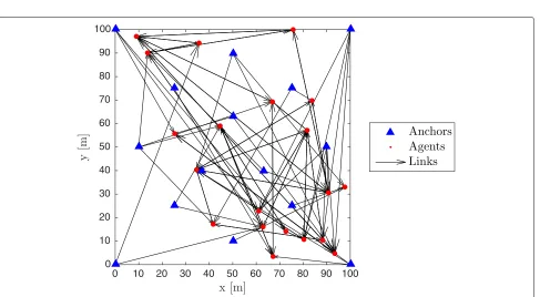
Figures 1 and 2 show two examples of RDML-initializable graphs. Figure1illustrates the case of a small (Na = 4,Nu = 4) but highly connected network. In
con-trast, Fig. 2 displays a larger (Na = 15,Nu = 20), but
weakly connected network (graph depth= 7). In partic-ular, only 90 out of 680 possible directed links are con-nected, where anchors have three to four links (out of 20). For both cases, graph compatibility can be shown using Algorithm 3.
4 Results and discussion
In this section, we use standard Monte Carlo (MC) sim-ulation to evaluate the performance of the proposed algorithm and its competitors. As a performance metric,
Algorithm 3Graph Compatibility Test
Input: Directed GraphGwithV =Va∪Vu Output: Binary flagfG, DepthhG
Initialization:
1: SetColor(Vu)←0; %white 2: fori=1 to|Vu|do 3: if|a(i)| ≥3then 4: Color(i)←1; %black
5: end if
6: end for
7: Initialize setˆu(0)(i)for every agentiand setB(u0); 8: ComputeCG(0) = B(u0);ifCG(0) = |Vu|,stopand
return(fG,hG)=(1, 0);
Coloring Loop
9: Setk←1; 10: while(1)do
11: fori=1 to|Vu|do
12: if|a(i)| + | ˆu(k−1)(i)| ≥3then 13: Color(i)←1;
14: end if
15: end for
16: Update ˆu(k)(i) for every agent i and compute
CG(k)← |B(uk)|;
Exit condition
17: ifCG(k−1)=CG(k)then 18: hG←k−1;
19: ifCG(k) <|Vu|then
20: fG←0; %graph G is RDML-incompatible 21: else
22: fG←1; %graph G is RDML-compatible
23: end if
24: breakloop;
25: end if
26: k←k+1;
27: end while
28: return fG,hG.
we will show the ECDF (empirical cumulative distribu-tion funcdistribu-tion) of the localizadistribu-tion error, defined as ei xˆi−xifor agenti, i.e., an estimate of the probability
Pxˆi−xi≤γ . The ECDFs are obtained by stacking
all the localization errors for every agent in a single vec-tor, in order to give a global picture of the algorithm performances. The simulated scenario is as follows. In a square coverage area of 100×100 m2,Na=11 stationary
anchors are deployed, as depicted in Fig.3. The channel parameters are generated as follows:p0LOS ∼ U[−30, 0],
αLOS ∼ U[ 2, 4], andσLOS = 6, while, for the NLoS case,
Fig. 1Example of a compatible graph withNa=4,Nu=4
Fig. 3Anchors positions used in all simulations
MC trial,Nu=10 agents are randomly (uniformly)
gener-ated in the coverage area. Unless stgener-ated otherwise,K=40 samples per link are used. Finally, each simulation consists of 100 MC trials.
The optimization problems (27) and (19) have been solved as follows. For DML, a 2D grid search has been used, while, for RDML and C-MLE, the opti-mization has been performed with the MATLAB solver
fmincon.
4.1 Gaussian noise
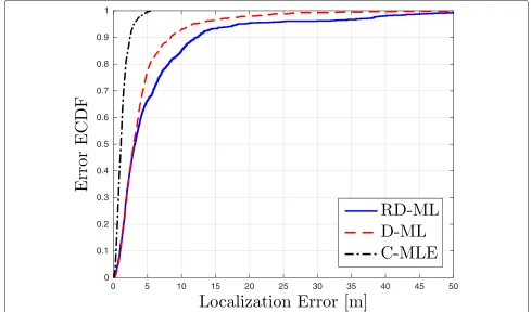
Here, we validate our novel approach by considering fully connected networks in three different scenarios. In Fig.4, all links are assumed to be LoS. As can be seen from the ECDFs, the robust approach has similar performances to the D-ML algorithm, which was designed assuming all links to be of the same type. In Fig.5, all links are assumed to be NLoS and again we see a similar result. The key difference is in Fig.6, where a mixed LoS/NLoS scenario is considered and the fraction of NLoS links is random (numerically generated as U[ 0, 1] and different for each MC trial). Here, the robust approach outperforms D-ML, validating our strategy. Moreover, it has a remarkably close performance to the centralized algorithm C-MLE. As a result, the robust approach is the preferred option in all scenarios.
4.2 Non-Gaussian noise for NLoS
In order to evaluate robustness, we consider a model mismatch on the noise distribution by choosing, for the NLoS links, a Studenttdistribution withν = 5 degrees of freedom (as usual, serially i.i.d. and independent from the LoS noise sequence). For brevity, we consider only the case of a fully connected network in a mixed LoS/NLoS scenario. As shown by Fig. 7, our proposed approach is able to cope with non-Gaussianity without a significant performance loss, thanks to the Gaussian mixture model.
4.3 Cooperative gain
The proposed algorithm exhibits the so called “cooper-ative gain,” i.e., a performance advantage (according to some performance metric, typically localization accuracy) with respect to a non-cooperative approach, where each node tries to localize itself only by self-localization (12). In our case, the cooperative gain is twofold: first, it allows to improve localization accuracy; second, it allows to local-ize otherwise non-localizable agents. To show the first point, we consider a mixed LoS/NLoS environment (for simplicity, with white Gaussian noise) and a network is generated at each Monte Carlo trial, assuming a commu-nication radiusR = 70 m, with an ideal probability of detection model [17]. Moreover, the network is generated in a way as to allow all agents to self-localize and, as a
Fig. 6Mixed LoS/NLoS scenario with white Gaussian noise. Fully connected networks, randomized NLoS fraction,Na=11,Nu=10
Fig. 8Cooperative (RDML) and non-cooperative approaches in a mixed LoS/NLoS scenario, in a network with communication radiusR=70 m, Na=11,Nu=10
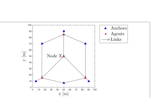
consequence, it is RDML-compatible. In Fig.8, the ECDFs of the localization error are shown. To show the second point, we consider the toy network depicted in Fig.9. In this example, agent X is not able to self-localize, since no anchors are in its neighborhood,a(X) = ∅. Thus,
in a non-cooperative approach, the position of agent X cannot be uniquely determined7, while, in a cooperative approach, the position of agentXcan actually be obtained by exchanging information, e.g., the estimated positions of its neighbors.
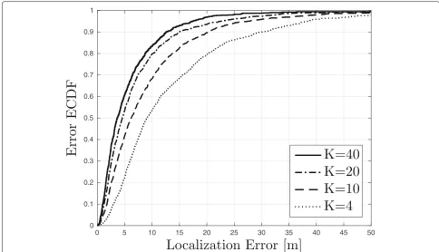
4.4 VariableKand NLoS fraction
We next analyze the RDML algorithm by varying the number of samples per link, K, and the frac-tion of NLoS links. In both cases, we consider (for brevity) fully connected networks with white Gaussian noise; for variable K, the fraction of NLoS is random-ized, while, for variable NLoS fraction, K is fixed. In Fig. 10, we observe that the performance increases as K increases, as expected. In Fig. 11, where each point represents 100 MC trials, the median error is chosen as a performance metric8 and RDML shows good per-formances and is not significantly affected by the actual NLoS fraction, which is evidence for its robustness, while D-ML is clearly inferior and suffers from model mismatch.
4.5 Communication and computational costs
The communication overhead is evaluated by comput-ing the number ofelementary messagessent throughout the network, where an elementary message is simply defined as a single scalar. Sending ad-dimensional mes-sage, e.g., (x,y) coordinates, is equivalent to sending d elementary messages. In Fig.12, the communication over-head of RDML and DML is plotted with respect to the number of agents, assuming a complete graph: for Nu
agents, 2Nu(Nu −1)scalars, representing estimated 2D
positions, are needed for RDML, while 4Nu(Nu − 1)
are needed for DML, as estimates of (p0,α) are also
necessary. Viewing (2D) position has the fundamen-tal information of a message (d = 2), in a com-plete graph, RDML achieves the theoretical minimum cost in order for all nodes to have complete informa-tion, while DML uses auxiliary information. For a gen-eral graph, the communication overhead depends on the specific graph topology, but is never greater than the aforementioned value. Thus, for a general graph, the communication cost is upper-bounded by a quadratic function ofNu.
Regarding computational complexity, both RDML and DML scale linearly with Nu and they benefit from
par-allelization, as the main optimization task can be exe-cuted independently for each involved node. As already
Fig. 11Median error of RDML and D-ML for a variable fraction of NLoS links. Fully connected networks,K=40,Na=11,Nu=10
mentioned, DML operates a trade-off between commu-nication and computational complexity; in fact, the DML optimization problem (27) is easier to solve than the RDML optimization problem (19). Both problems are non-convex and may have local minima/maxima, so care must be taken in the optimization procedure.
5 Conclusions
We have developed a novel, robust ML-based scheme for RSS-based distributed cooperative localization in mixed LoS/NLoS scenarios, which, while not being optimal, has good overall accuracy, is adaptive to the environment changes, is robust to NLoS propagation, including non-Gaussian noise, and has communication overhead upper-bounded by a quadratic function of the number of agents and computational complexity scal-ing linearly with the number of agents, also benefitscal-ing from parallelization. The main original contributions are that, unlike many algorithms present in the literature, the proposed approach (a) does not require calibration and (b) does not require symmetrical links (nor does it resort to symmetrization), thus naturally accounting for the topol-ogy of directed graphs with asymmetrical links as a result of miss-detections and channel anisotropies. To the best of the authors’ knowledge, this is the first distributed cooperative RSS-based algorithm fordirectedgraphs. The main disadvantage is imposing some restrictions on the arbitrariness of networks’ topology, but these restrictions disappear for sufficiently connected networks. We also derive a compatibility test based on graph coloring, which allows to determine whether the given network is com-patible. If it is compatible, convergence of the algorithm is guaranteed. Future work may include the considera-tion of possible approximaconsidera-tions, in order to extend this approach to more general networks, and of alternative models, overcoming the limitations of the standard path loss model.
Endnotes
1Throughout the paper, vectors and matrices will be
denoted in bold,vdenotes the Euclidean norm of vec-torv,|A|denotes the cardinality of setA. We denote by E[X] and Var[X] the statistical expectation and variance, respectively, of random variableX. Finally,B = {0, 1}is the Boolean set.
2The values on the main diagonal are arbitrary. Here we
choosemi→i=1. 3δ
i,j=1 if and only ifi=j, zero otherwise.
4For better readability, the notation (m) has not been
carried over, as it implicit in the formalism.
5The reason for this is that localizing a node in 2D
requires at least three anchors.
6Hereafter, we omit the conditioning on the set{o n→i}
of actually observed RSS measures (received by node i) in the joint likelihood function, since it is implicit in the neighborhood formalism.
7This easily follows by observing that the deterministic
(noiseless) version of all the relevant equations for agent Xadmit infinite solutions.
8This is due to the fact that RSME (Root Mean Square
Error) is not a suitable metric when the Error ECDFs are very long-tailed, as in our case.
6 Appendix A: On using the time-averaged sample mean
Let ⊆ Rd be the (non-empty) parameter space, θ ∈ unknown deterministic parameters ands : → Ra function. Consider the following model
y(k)=s(θ)+w(k), w(k)∼N0,σ2 (32)
where k = 1,. . .,K and the noise sequence w(k) is zero-mean, i.i.d. Gaussian, with deterministic unknown varianceσ2>0. Let the joint likelihood function. Then,
arg max
ProofSince the observations are independent,
py(1),. . .,y(k);θ,σ2=
Observing now that
Thus, the joint pdf can be factorized as follows
py(1),. . .,y(k);θ,σ2
As a by-product, by invoking the Neyman-Fisher fac-torization theorem [45] and assuming knownσ2, y¯ is a sufficient statistic forθ. Resuming our proof, we can now observe that
since no term in the summation depends onk. Thus,
arg max
7 Appendix B: C-MLE derivation The MLE ofxis given by
ˆ
xML=arg max
x p(ϒ;x) (43)
where p(ϒ;x) is the joint likelihood function. Since all other parameters are assumed known, the set of all time-averaged measuresϒ¯ = ∪Nu
i=1Y¯iis a sufficient statistic for
x(see AppendixA), from which it follows that
arg max
Taking the natural logarithm and neglecting constants,
ˆ
BP: Belief propagation; C-MLE: Centralized maximum likelihood estimator; D-ECM: Distributed expectation-conditional maximization; DML: Distributed maximum likelihood; ECDF: Empirical cumulative distribution function; ECM: Expectation-conditional maximization; EM: Expectation-maximization; LoS: Line-of-sight; LS: Least squares; MC: Monte Carlo; ML: Maximum likelihood; MLE: Maximum likelihood estimator; NBP: Nonparametric belief propagation; NLoS: Non-line-of-sight; RDML: Robust distributed maximum likelihood; RF: Radiofrequency; RMSE: Root mean square error; RSS: Received signal strength; RSSI: Received signal strength indicator; SDP: Semidefinite-programming; SPAWN: Sum-product algorithm over wireless networks; WLS: Weighted least squares; WSN: Wireless sensor network; 2D: 2-dimensional
Acknowledgements
The authors would like to thank prof. F. Bandiera from University of Salento for having started the collaboration which lead to this work.
Funding
The work of L. Carlino was supported by the “Erasmus+ Traineeship” programme of University of Salento. The work of M. Muma was supported by the “Athene Young Investigator Programme” of Technische Universität Darmstadt.
Availability of data and materials
The datasets used and/or analyzed during the current study are available from the corresponding author on reasonable request.
Authors’ contributions
Authors’ information
LCreceived his B.Sc. degree with full marks in Information Engineering at University of Salento, Lecce, Italy, in 2012. He received his M.Sc. degree in Telecommunications Engineering (summa cum laude) at University of Salento, in 2014. He started his Ph.D. studies at University of Salento in 2014 and finished his Ph.D. in 2018. His main area of research is signal processing, while his research topic is applying signal processing techniques to the problem of localization, with a specific focus on localization based upon received signal strength. His other research interests include radar applications, target tracking, data mining and information theory.
DJreceived the B.Sc. degree in information and communication engineering from Zhejiang University, Hangzhou, China, in 2011, and the M.Sc. degree in electrical engineering and information technology from Technische Universität Darmstadt, Darmstadt, Germany, in 2014. She is currently working towards the Ph.D. degree in the Signal Processing Group at Technische Universität Darmstadt. Her research interests include localization and tracking, distributed and cooperative inference in wireless networks.
MMreceived the Dipl.-Ing (2009) and the Dr.-Ing. degree (summa cum laude) in Electrical Engineering and Information Technology (2014), both from Technische Universität Darmstadt, Darmstadt, Germany. He completed his diploma thesis with the Contact Lens and Visual Optics Laboratory, School of Optometry, Brisbane, Australia, on the role of cardiopulmonary signals in the dynamics of the eye’s wavefront aberrations. Currently, he is a Postdoctoral Fellow at the Signal Processing Group, Institute of Telecommunications and has recently been awarded Athene Young Investigator of Technische Universität Darmstadt. His research is on robust statistics for signal processing with applications in biomedical signal processing, wireless sensor networks, and array signal processing. MM was the supervisor of the Technische Universität Darmstadt student team who won the international IEEE Signal Processing Cup 2015. MM co-organized the 2016 Joint IEEE SPS and EURASIP Summer School on Robust Signal Processing. In 2017, together with his coauthors, MM received the IEEE Signal Processing Magazine Best Paper Award for the paper entitled “Robust Estimation in Signal Processing: A tutorial-style treatment of fundamental concepts". In 2017, he was elected to the European Association for Signal Processing (EURASIP) Special Area Team in Theoretical and Methodological Trends in Signal Processing (SAT-TMSP). AZis a Fellow of the IEEE and IEEE Distinguished Lecturer (Class 2010- 2011). He received his Dr.-Ing. from Ruhr-Universität Bochum, Germany in 1992. He was with Queensland University of Technology, Australia from 1992–1998 where he was Associate Professor. In 1999, he joined Curtin University of Technology, Australia as a Professor of Telecommunications. In 2003, he moved to Technische Universität Darmstadt, Germany as Professor of Signal Processing and Head of the Signal Processing Group. His research interest lies in statistical methods for signal processing with emphasis on bootstrap techniques, robust detection and estimation and array processing applied to telecommunications, radar, sonar, automotive monitoring and safety, and biomedicine. He published over 400 journal and conference papers on the above areas. AZ served as General Chair and Technical Chair of numerous international conferences and workshops; more recently he was the Technical Co-Chair of ICASSP-14 held in Florence, Italy. He also served on publication boards of various journals, notably as Editor-In-Chief of the IEEE Signal Processing Magazine (2012–2014). AZ was the Chair (2010–2011) of the IEEE Signal Processing Society (SPS) Technical Committee Signal Processing Theory and Methods (SPTM). He served on the Board of Governors of the IEEE SPS (2015–2017) and is the president of the European Association of Signal Processing (EURASIP) (2017–2018).
Competing interests
The authors declare that they have no competing interests.
Publisher’s Note
Springer Nature remains neutral with regard to jurisdictional claims in published maps and institutional affiliations.
Author details
1Department of Innovation Engineering, University of Salento, Lecce, Italy. 2Signal Processing Group, Department of Electrical Engineering and
Information Technology, Technische Universität Darmstadt, Darmstadt, Germany.
Received: 27 September 2018 Accepted: 21 December 2018
References
1. F. Gustafsson, F. Gunnarsson, Mobile positioning using wireless networks. IEEE Signal Process. Mag.22(4), 41–53 (2005)
2. N. Patwari, J. Ash, S. Kyperountas, A. O. I. Hero, R. Moses, N. Correal, Locating the nodes: Cooperative localization in wireless sensor networks. IEEE Signal Process. Mag.22(4), 54–69 (2005)
3. S. Gezici, A survey on wireless position estimation. Wireless Pers. Commun.44(3), 263–282 (2008)
4. L. M. Trevisan, M. E. Pellenz, M. C. Penna, R. D. Souza, M. S. Fonseca, A simple iterative positioning algorithm for client node localization in WLANs. EURASIP Wireless, J. Commun. and Netw.2013(1), 276 (2013) 5. A. Coluccia, F. Ricciato, A Software-defined radio tool for experimenting
with RSS measurements in IEEE 802.15.4: implementation and applications. Int. Sensor J. Netw.14(3), 144–154 (2013)
6. T. S. Rappaport,Wireless Communications: Principles and Practice (2nd Ed.) (Prentice Hall, Upper Saddle River, NJ, USA, 2002)
7. J. Koo, H. Cha, Localizing WiFi access points using signal strength. IEEE Commun. Lett.15(2), 187–189 (2011)
8. A. Matic, A. Papliatseyeu, V. Osmani, O. Mayora-Ibarra, inProc. 8th IEEE Int. Conf. Pervasive Comput. Commun. (PerCom). Tuning to your position: FM radio based indoor localization with spontaneous recalibration, (Mannheim, Germany, 2010), pp. 153–161
9. M. Hellebrandt, R. Mathar, M. Scheibenbogen, Estimating position and velocity of mobiles in a cellular radio network. IEEE Trans. Veh. Technol. 46(1), 65–71 (1997)
10. F. Yin, A. Li, A. M. Zoubir, C. Fritsche, F. Gustafsson, inIn Proc. 5th IEEE Int. Workshop Computat. Adv. Multi-Sensor Adapt. Process. (CAMSAP). RSS-based sensor network localization in contaminated Gaussian measurement noise, (2013), pp. 121–124
11. F. Bandiera, A. Coluccia, G. Ricci, A. Toma, inProc. 39th IEEE Int. Conf. Acoust. Speech Signal Process. (ICASSP). RSS-based localization in
non-homogeneous environments, (Florence, Italy, 2014), pp. 4247–4251 12. F. Bandiera, A. Coluccia, G. Ricci, A Cognitive Algorithm for Received
Signal Strength Based Localization. IEEE Trans. Signal Process.63(7), 1726–1736 (2015)
13. F. Bandiera, L. Carlino, A. Coluccia, G. Ricci, inProc. IEEE 6th International Workshop Comput. Adv. Multichannel Sensor Array Process. (CAMSAP). RSS-based localization of a moving node in homogeneous environments, (Cancun, Mexico, 2015), pp. 249–252
14. F. Bandiera, L. Carlino, A. Coluccia, G. Ricci, inProc. 19th Int. Conf. Inform. Fusion (FUSION). A cognitive algorithm for RSS-based localization of possibly moving nodes, (2016), pp. 2186–2191
15. S. Tomic, M. Beko, R. Dinis, Distributed RSS-AOA Based Localization With Unknown Transmit Powers. IEEE Wireless Commun. Lett.5(4), 392–395 (2016)
16. P. Abouzar, D. G. Michelson, M. Hamdi, RSSI-Based Distributed Self-Localization for Wireless Sensor Networks Used in Precision Agriculture. IEEE Trans. Wireless Commun.15(10), 6638–6650 (2016) 17. R. Zekavat, R. M. Buehrer,Handbook of Position Location: Theory, Practice,
And Advances. (Wiley-IEEE press, Hoboken, 2011)
18. L. Y., F. S., G. D., C. K., inProc. 6th IEEE Int. Sympos. Microw., Ant., Prop., EMC Technol. (MAPE). A non-cooperative localization scheme with unknown transmission power and path-loss exponent, (2015), pp. 720–725 19. D. Jin, F. Yin, C. Fritsche, A. M. Zoubir, F. Gustafsson, inProc. 41st IEEE Int.
Conf. Acoust. Speech Signal Process. (ICASSP). Cooperative localization based on severely quantized RSS measurements in wireless sensor network, (2016), pp. 4214–4218
20. S. Tomic, M. Beko, R. Dinis, RSS-Based Localization in Wireless Sensor Networks Using Convex Relaxation: Noncooperative and Cooperative Schemes. IEEE Trans. Veh. Technol.64(5), 2037–2050 (2015) 21. F. Yin, C. Fritsche, F. Gustafsson, A. M. Zoubir, inProc. 38th IEEE Int. Conf.
Acoust. Speech Signal Process. (ICASSP). Received signal strength-based joint parameter estimation algorithm for robust geolocation in LOS/NLOS environments, (2013), pp. 6471–6475
22. F. Yin, C. Fritsche, D. Jin, F. Gustafsson, A. M. Zoubir, Cooperative localization in WSNs using Gaussian mixture modeling: Distributed ECM algorithms. IEEE Trans. Signal Process.63(6), 1448–1463 (2015) 23. A. T. Ihler, J. W. Fisher, R. L. Moses, A. S. Willsky, Nonparametric belief
propagation for self-localization of sensor networks. IEEE Sel, J., Areas Commun.23(4), 809–819 (2005)
25. F. Scheidt, D. Jin, M. Muma, A. M. Zoubir, inProc. 24th European Signal Process. Conf. (EUSIPCO). Fast and accurate cooperative localization in wireless sensor networks, (2016), pp. 190–194
26. D. Jin, F. Yin, C. Fritsche, A. M. Zoubir, F. Gustafsson, inProc. 23rd European Signal Process. Conf. (EUSIPCO). Efficient cooperative localization algorithm in LOS/NLOS environments, (2015), pp. 185–189
27. N. Patwari, A. O. Hero, M. Perkins, N. S. Correal, R. J. O’Dea, Relative Location Estimation in Wireless Sensor Networks. IEEE Trans. Signal Process.51(8), 2137–2148 (2003)
28. R. W. Ouyang, K.-S. A.Wong, C.-T. Lea, Received Signal Strength-Based Wireless Localization via Semidefinite Programming: Noncooperative and Cooperative Schemes. IEEE Trans. Veh. Technol.59(3), 1307–1318 (2010) 29. H. Lim, L. C. Kung, J. C. Hou, H. Luo, inProc. 25th IEEE Int. Conf. Computer
Commun. (INFOCOM). Zero-configuration, robust indoor localization: theory and experimentation, (Barcelona, 2006), pp. 1–12
30. A. Coluccia, F. Ricciato, inProc. IEEE Int. Sympos. Wireless Pervasive Comput. (ISWPC). On ML estimation for automatic RSS-based indoor localization, (Modena, 2010), pp. 495–502
31. J. Riba, A. Urruela, inProc. 29th IEEE Int. Conf. Acoust. Speech Signal Process. (ICASSP), vol. 2. A non-line-of-sight mitigation technique based on ML-detection, (2004)
32. S. Gezici, Z. Sahinoglu,UWB geolocation techniques for IEEE 802.15.4a personal area networks, (Cambridge, 2004). TR-2004-110
33. J. J. Caffery, G. L. Stuber, Overview of radiolocation in CDMA cellular systems. IEEE Commun. Mag.36(4), 38–45 (1998)
34. S. Venkatesh, R. M. Buehrer, NLOS mitigation using linear programming in ultrawideband location-aware networks. IEEE Trans. Veh. Technol.56, 3182–3198 (2007)
35. X. Wang, Z. Wang, B. O’Dea, A TOA-based location algorithm reducing the errors due to non-line-of-sight (NLOS) propagation. IEEE Trans. Veh. Technol.52(1), 112–116 (2003)
36. R. Casas, A. Marco, J. J. Guerrero, J. Falcó, Robust estimator for non-line-of-sight error mitigation in indoor localization. EURASIP Adv, J., Signal Process.2006(1), 043429 (2006)
37. G.-L.S., W.G., Bootstrapping M-estimators for reducing errors due to non-line-of-sight (NLOS) propagation. IEEE Commun. Lett.8(8), 509–510 (2004)
38. D. Liu, Y. Wang, P. He, Y. Zhai, H. Wang, TOA localization for multipath and NLOS environment with virtual stations. EURASIP Wireless, J., Commun. and Netw.2017(1), 104 (2017)
39. F. Yin, C. Fritsche, F. Gustafsson, A. M. Zoubir, TOA-based robust wireless geolocation and Cramér-Rao lower bound analysis in harsh LOS/NLOS environments. IEEE Trans. Signal Process.61(9), 2243–2255 (2013) 40. S. D. Chitte, S. Dasgupta, Z. Ding, Distance estimation from received signal
strength under log-normal shadowing: bias and variance. IEEE Signal Process. Lett.16(3), 216–218 (2009)
41. A. Coluccia, Reduced-bias ML-based estimators with low complexity for self-calibrating RSS ranging. IEEE Trans. Wireless Commun.12(3), 1220–1230 (2013)
42. C. Savarese, J. M. Rabaey, J. Beutel, inProc. 26th IEEE Int. Conf. Acoust. Speech Signal Process. (ICASSP). Location in distributed ad-hoc wireless sensor networks, vol. 1, (2001), pp. 2037–2040
43. C. Savarese, J. M. Rabaey, K. Langendoen, inProc. Gen. Track Ann. Conf. USENIX Ann. Techn. Conf, ATEC ’02. Robust positioning algorithms for aistributed ad-hoc wireless sensor networks (USENIX Association, Berkeley, 2002), pp. 317–327
44. A. Savvides, C.-C. Han, inProc. 7th Ann. Int. Conf. Mobile Comput. Netw. (MobiCom). MobiCom ’01. M.B.S.: Dynamic fine-grained localization in ad-hoc networks of sensors (ACM, New York, 2001), pp. 166–179 45. S. M. Kay,Fundamentals of Statistical Signal Processing: Estimation Theory.
(Prentice Hall, Englewood Cliffs, New Jersey, 1993)
46. L. Mihaylova, D. Angelova, D. Bull, N. Canagarajah, Localization of mobile nodes in wireless networks with correlated in time measurement noise. IEEE Trans. Mobile Comput.10(1), 44–53 (2011)