R E S E A R C H
Open Access
A map-matching algorithm with
low-frequency floating car data based on
matching path
Ling Yuan, Dan Li
*and Song Hu
Abstract
With the wide application and rapid development of Intelligent Transportation System (ITS), the floating car has been widely used in the collection of traffic information, which is also very important in the application of the wireless sensor networks. In addition to the high-frequency floating car, energy-saving low-frequency floating car has attracted great attention, but the low-frequency GPS data have a poor effect on map matching. Taking consideration of the distance, direction, speed, and topology of road and vehicle, we propose a global map matching algorithm with low-frequency floating car data based on the matching path. The proposed algorithm preprocesses the floating car data and road network data to determine the potential points and sections by constructing the error region. Then, we calculate the potential matching path graph with the analysis of time and space. Finally, we can obtain the matching result by parallel computing with section division methodology. The experiment results demonstrate that the proposed map-matching algorithm can improve the running time and matching accuracy compared with the existing methods.
Keywords:Low-frequency floating car data, Map matching, Potential point, Positioning point, Matching path
1 Introduction
In the application of the wireless sensor networks, traffic information from the senor is very important to control the traffic congestion. With the rapid development of economy, traffic congestion are getting worse, and at the same time, more and more technology has been applied to the traffic management, where the Intelligent Transpor-tation System (ITS) is a significant method [1]. ITS is a real-time, efficient, and comprehensive transportation management system which integrates advanced electronic technology and information technology. ITS makes a new way of interaction among three main traffic systems: car, road, and traffic, which can reduce traffic congestion to improve the traffic capacity [2,3]. The implementation of ITS system depends on the accurate and real-time traffic information.
At present, most of the traffic information is collected by floating car [4], which can acquire the vehicle’s pos-ition, speed, direction, and other information directly with low monitoring cost and high efficiency. The floating car
is an advanced method to obtain the traffic information. The floating car utilizes the vehicle GPS device to collect the vehicle position data information, then send the data information to the processing center with the wireless communication transmission technology. In the process-ing center, the map matchprocess-ing methodology is used to match the collected information and map information to obtain real-time traffic condition [5].
However, due to the complex city geographical features, when facing the viaduct, culverts, high-rise buildings, and other terrains, the positioning accuracy of floating car would be significantly reduced. In order to provide more accurate positioning data, it is necessary to process the corresponding correction to the data acquired by the floating car, where the map matching is the key technol-ogy to achieve this goal [6,7].
Map matching is also called map-aided positioning technology, which is based on the pattern recognition theory. We set the positioning information obtained by the positioning device as the objects to be matched and set the geographic information in electronic map as the matching template. With the calculation of similarity * Correspondence:[email protected]
Huazhong University of Science and Technology, Wuhan 430072, China
between the objects to be matched and the matching template, we can choose the correct vehicle travel matching path according to such similarity [8]. The map-matching technology is normally implemented in the field of traffic control. At present, most of the map-matching algorithms mainly aim at the high-frequency GPS data.
In practical applications, due to energy consumption and economic consideration, the data acquired by floating cars are low-frequency GPS data whose sampling time interval is more than 2 min. The sampling time interval of high-frequency GPS data is less than 2 min; two collected adjacent positioning points are generally located in a sec-tion of the road. For the low-frequency GPS data, with the increase of sampling time interval, in the complex city road network condition, the vehicle may pass through multiple complex sections, the matching effect and the matching efficiency will be affected greatly. To solve this problem, considering the distance, direction, speed, con-nectivity, and other factors, we propose a map-matching algorithm with the low-frequency floating car data, which can improve the accuracy and efficiency of map matching to select the correct matching path rapidly.
The paper is organized as follows. In Section2, we give the related work. The proposed map-matching algorithm with the low-frequency floating car data is presented in Section3. Experiment simulation and result analysis are il-lustrated in Section4and conclusion remarks in Section5.
2 Related work
Traditional map-matching algorithm is simple and fast, but with the construction and development of urban traffic, the urban road and the traffic condition are more and more complex, the traditional map-matching algo-rithm would produce inaccurate matching results. Therefore, many experts have an in-depth analysis and research about map-matching algorithm.
Bernstein and Kornhauser presented a geometric match-ing algorithm, mainly includmatch-ing the matchmatch-ing of point to point and point to the curve [9]. Geometric matching algo-rithm is the foundation to the map-matching algoalgo-rithm. Taylor proposed road reduction filter (RPF) algorithm, aiming at the map matching with positioning device GPS, which can improve the matching of point to the curve and curve to curve and the matching accuracy with differential GPS correction [10]. Greenfield proposed a map-matching algorithm based on network topology, which has used weighted method to fitting out multiple matching factors, and then selected the matching section. The experiments have demonstrated the significance of such algorithm [11]. Alt used Fréchet distance to measure the similarity be-tween the trajectory composed of positioning points and the road to be matched, where the similarity can be used as the standard to choose the matching path [12].
However, the complexity of the algorithm is a little high. Brakatsoulas improved such algorithm by replacing the Fréchet distance with the weak Fréchet distance, which can reduce the algorithm complexity [13].
Peng Fei put forward a map-matching technology based on probability and statistics, which can establish a confi-dence region based on the received positioning points to determine the matching sets quickly to improve the matching efficiency [14]. Gao Jian introduced a dynamic filtering technology into direct and indirect modes, which can process sections with shape and sections without shape efficiently. Such algorithm can achieve good effect in the simulation experiments [15]. Sinn Kim presented an adaptive fuzzy neural network map-matching algo-rithm. The algorithm calculated C-measure value for each positioning point, where C-measure considered the factor of distance and direction to indicate the probability of a vehicle traveling on a road section [16]. According to the characteristics of the floating car, Wang Xiaomeng pre-sented a map-matching algorithm based on hidden Mar-kov chain. This algorithm has many improvements compared with a traditional model: introducing heading variable into the calculation of emission probability and using the path distance to build the road transfer matrix of the activities range within the floating car moving scope. With these improvements, such map-matching al-gorithm has both high matching accuracy and high matching efficiency [17].
The current map-matching algorithms mainly aimed at vehicle positioning data with high frequency. There is few study of low-frequency data map matching. In 2013, Yao Enjian presented a real-time map-matching algo-rithm with low-frequency floating car data, called the piecewise fuzzy matching algorithm. The algorithm di-vided low-frequency positioning data collected by float-ing car at a fixed time interval (5 min). Considerfloat-ing the connectivity between two periods, the last locating point in the previous period has been taken as the starting point of the next period. Then the matching path can be calculated for each time period and connected to obtain the matching path for the floating car track [18]. In 2015, Shen Jingwei proposed a map-matching algorithm based on improved activity on edge (AOE) network with low-frequency floating car. The vertices in the graph were all the positioning points of the positioning points, and the edge weight was the path length of the potential points. The shortest path from the start to the end of the AOE graph was the matching path of the floating car track [19]. The experimental results showed that the algorithm has obvious advantages both at running time and matching accuracy compared with the global match-ing algorithm based on weak Fréchet distance.
calculation only considers the shortest path, making no use of other information which would affect the floating car track matching results, such as the direction of the floating car, the velocity of floating car, and the distance between the positioning points and the potential points. Our proposed map-matching algorithm will make full use of the information gathering by floating car to im-prove the matching effect highly.
3 Map-matching algorithm
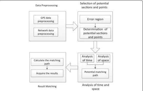
The whole framework of the proposed map-matching al-gorithm is shown in Fig.1, which consists of four mod-ules: The first one is the GPS data and road network data preprocessing, which can sift out the redundant data and abnormal data collected by floating car and construct the topology structure and grid partition, illus-trated in Section 3.1; the second one is the selection of potential road sections and potential points, which can filter out the potential road sections according to error region built by the theory of probability and statistics, the vehicle’s speed, and the angle of vehicle direction and road direction, illustrated in Section 3.2; the third one is the time-space analysis for positioning points, cor-responding potential points, and potential matching seg-ments to obtain the potential matching path map of
floating vehicle trajectory, illustrated in Section 3.3; the fourth one is the results matching, where one matching path of potential matching path map is the matching path of the floating vehicle, illustrated in Section3.4.
Before illustrating these four modules in detail, we firstly define the map-matching problem.
Defining the trajectory T of GPS,T is a series of or-derly GPS positioning pointsp1,p2, …,pn, and the
infor-mation contained in each GPS positioning point can be expressed as (pi. lat,pi. lng,pi. time,pi. v,pi. β), corre-sponding to the longitude, latitude, time, the instantan-eous velocity, and the moving direction angle of positioning point, respectively.
Defining the road networkG(V, E),G(V, E)can be rep-resented with a directed graph;Vis a collection of start-ing point, endstart-ing point, intersection point, and shape point in a road network; and Eis a collection of section in road network. Each sectioneis a directed edge, which can be expressed as a (e.id,e.v,e.l,e.start,e.end), cor-responding to the serial number of section, the speed limit, the length of the road, the starting point, and the ending point of the section, respectively.
Defining the path P, the given two points viandvjon the network, P is a collection of connected sections starting fromviand ending invj.
Then the map-matching problem can be defined as follows: with the road networkGand untreated GPS tra-jectoryT, it is to solve the actual path ofTinG.
3.1 Data preprocessing
3.1.1 GPS data preprocessing
As the urban road network condition is very complex, when floating car drives in a tunnel, under the overpass or meet with larger building block, it will cause the devi-ation of GPS data. In addition, the vehicle low-speed driving or parking, caused by the traffic congestion or vehicle failure, will produce a lot of redundant data. These abnormal data and redundant data will seriously affect the effective execution of map-matching algo-rithm. Therefore, before matching the GPS positioning points, we preprocess the GPS data as follows:
1. Delete the data according to the space limit; 2. Delete the data according to the speed limit
threshold;
3. Delete the data according to the static data drift.
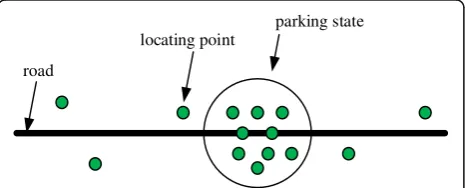
When the speed is slow or the vehicle stops, the posi-tioning point theoretically should be in dense distribution along the road or gathered at a point. But because of the GPS positioning deviation, it will make the positioning point present as a random fluctuation phenome taking a point as the center, as shown in Fig.2. Since these points are close to each other, they can be filtered out according to the distance. If the velocity of the floating car in current locating point is low (v< 3 m/s) and the distance between the current positioning point and the previous positioning point is less than the threshold, we can ignore the current positioning point and take the previous positioning point as the current positioning point.
3.1.2 Network data preprocessing
For road information, in addition to the storage of nodes, shape point, and road section, we also need to store the connection information between them, namely the topology information. To build a network topology relationship, we need to consider the relationship be-tween nodes, relationship bebe-tween node and section
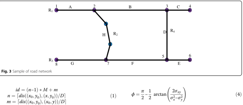
node, and link relationship between section and section. Figure3 is a simple road network, including four paths: R1, R2, R3, and R4. These paths are divided by nodes into eight sections, sections A, B, C, D, E, F, G, and H, where the purple dot presents the road intersection node, and the blue dot presents the shape point in the section.
We can build the road topology according to the fol-lowing steps:
1. Reading the road R1, finding the starting point, end point of R1, and the intersection points with other roads, numbering these nodes following the sequence starting from number 1, then generating the node link table. Taking into account the road direction, one-way street only takes a row of re-cords in the table, while two-way street takes two rows of records.
2. Processing road R2~R4 as R1 in turn. If road nodes have serial number, we can use the existing serial number, if not, order number in sequence and add them to the node links table.
3. Sorting the node link table according to the starting point of the section to obtain a new node link table. 4. Merging all records with the same starting point
number in the node link table to build the
topological relations between nodes and nodes, and nodes and links.
5. For two-way road section, finding out the associated sections with similar starting point or end point from the node link table. For one-way road section, finding out the associated sections with the similar end point in the node link table. Then merging the same section to obtain the topological relations be-tween sections.
After building the road network topology, we process the road network with grid partition to associate each grid with the sections in each grid area, which can help the rapid fil-tering out potential sections of positioning points. Due to the high accuracy of current GPS positioning, the actual lo-cation of the floating car should be in the road section within 100-m distance to the positioning point. Therefore, we chooseD= 100 m as the length of grid side. Taking the length and width of electronic map as L andW, respect-ively, we divide the electronic map with the square whose side isDinto the number ofM*Ngrids; therefore,M=⌈L/
D⌉, andN=⌈W/D⌉. We can number the gird in the elec-tronic map from top to bottom, from left to right in se-quence. Assuming that the latitude and longitude coordinates of the positioning point is (x,y), the latitude and longitude coordinates of the point which is located in the upper left in the electronic map is (x0,y0), then the grid idof the positioning point can be calculated like this:
road
locating point
parking state
id¼ðn−1Þ Mþm n¼ddis xðð 0;y0Þ;ðx;y0ÞÞ=De m¼ddis xðð 0;y0Þ;ðx0;yÞÞ=De
ð1Þ
where dis is the Euclidean distance between two points. Considering the positioning point on the edge of the grid, the positioning point’s potential road sec-tion is fixed within nine grids centered with the posi-tioning point grid. After grid partition, we need to filter out the road sections in these nine grids, which can improve the efficiency of filtrating the potential road section greatly.
3.2 Selection of potential sections and potential points
3.2.1 Determination of error region
After grid partition, taking all road sections in nine grids centered to the positioning point grid as the potential road sections, which would lead to too many potential road sections. Taking advantage of the theory of probability and statistics to construct the error region of the positioning point can further re-duce the number of the potential sections. Because of the existence of various errors, all possible locations obtained by the vehicle GPS receiver present normal distribution in an area. According to the theory of probability and statistics, we can build an error model with the data obtained by positioning sensor, to gain the confidence region of vehicle real position. Ac-cording to the variance and covariance parameters of GPS receiver, the error confidence region can be de-fined as the ellipse form as below:
a¼σ0
In the above three formulas, ais the long semi-axis of the error ellipse, b is the short semi-axis error of the error ellipse, and ϕ is the angle between the long semi-axis and the north direction; σx and σy are the standard deviation of positioning point in the direction of north and east, which can be available in the output message of the GPS receiver; σxy is the covariance; and σ0is called the extended factor. When the shape is kept
constant by adjusting the value of σ0, the error ellipse
can be magnified and reduced to get different confidence level. When σ0= 1, the confidence level is 39%; whenσ0
= 2.15, the confidence level is 95%; and when σ0= 3.30,
the confidence level is 99% [20]. The center of the error ellipse is set as the positioning point.
3.2.2 Determination of potential sections and potential points
After getting the error region of the positioning point, the potential road section of the positioning point can be quickly screened out by judging whether the sections in the positioning point grid and the surrounding grid are located in the error region of the positioning point. The process of determination of potential sections and potential points is illustrated in Fig. 4. The potential points corresponding to the positioning points are the projection points on the corresponding potential sec-tions. We select the projection points according to the following method: if the projection point of the GPS po-sitioning point in the potential section is located in the potential section, select the projection point as the po-tential point of GPS positioning point and if the projec-tion point of GPS posiprojec-tioning point in the potential section is located in the potential section’s extension line, select the nearest node of the potential section to GPS positioning point as the potential point. Taking into account the angle between the direction of the floating
1 2 3 4
car and the direction of the potential section, the poten-tial section can be selected twice, in order to reduce the number of invalid candidates. According to the research results of Ochieng et al. [21], when the speed v of the floating car is less than 3 m/s, the direction angleθ will become unstable. Therefore, the rules for potential sec-tion to be screened out twice are as follows:
1. Whenv≥3m/s, the direction angle was limited toθ < 30°.
2. Whenv< 3m/s, the direction angle was limited toθ < 120°.
When two nodes n1(x1,y1), n2(x2,y2) on a potential
section are known, the direction angleаof the potential section can be calculated according to formula (5):
a¼
The direction angle β of the floating car can be ob-tained directly from the information of the positioning point. It can be concluded that the angle θbetween the direction of the vehicle and the potential section can be calculated as:
θ¼ 360−jα−βjα−β ;jα−βj≤180 j j ;jα−βj>180
ð6Þ
The screening process is shown in Fig. 5, and in the error region, we can obtain three potential sections L1,
L2, and L3, where the floating car speed of positioning pointPis 6 m/s.
When we process the secondary screening according to the direction angle, since the angle between the direc-tion of roadL3and the positioning pointPis larger than
30°, L3will be rejected from the potential sections. The final potential sections of pointPareL1andL2, and the corresponding matching points are c11 and c21, respect-ively. With the secondary screening, the invalid potential sections are discarded, which can reduce the number of potential points corresponding to the positioning point.
3.3 Analysis of time and space
The analysis of time and space is the core module of the proposed map-matching algorithm. By considering the time and space factors in the map matching, we can cal-culate the matching path map of the floating vehicle tra-jectory from the potential sections. Time and space analysis is based on the following three rules:
1. If there is no direct connection between two positioning points, the actual route of the floating car tends to choose the shortest path between the two positioning points. Taking the taxi as the research object of the floating car, under the urban road network, it will choose the shortest route. 2. The actual route of a floating car tends to be
straight rather than circuitous.
3. The speed of a floating car obeys the speed limit of the road network.
3.3.1 Analysis of space
In the space analysis, we calculate the observation ability of each potential point and the transition prob-ability between potential point pairs based on distance, direction, and topology connectivity. Observation prob-ability represents the possibility that potential points would be matching points based on the distance be-tween the positioning point and the potential point, the angle between the direction of the vehicle, and the road direction of the potential point. The transition probabil-ity represents the possibilprobabil-ity of the path between poten-tial point pairs as the actual path of two adjacent positioning points.
Determining of Potential Sections and
Points
Fig. 4Determining of potential sections and points
L1
The observation probability is defined as a probability that positioning point Pimatches to the potential point
cij. Our proposed calculation of observation probability not only considers the distance between the positioning point and the potential point, but also takes into account the angle between the direction of the floating car and the direction of the potential road section, which can improve the accuracy of the observation probability.
Generally, the distance between positioning point Pi and potential pointcijobeys the normal distribution with a mean value of 0. The angle θij between the floating car’s direction on positioning point Pi and the direction of the potential road Lj obeys the exponential distribu-tion. Therefore, the probability function of distancedijis expressed as formula (7), and the probability function of direction angleθijis expressed as formula (8).
fd cij ¼ ffiffiffiffiffiffi1
In formula (7), σis the standard deviation of the nor-mal distribution that distancedij is satisfied with. In for-mula (8), λ is the parameter with the exponential distribution that direction angleθijis satisfied with. Tak-ing into account the distance and direction angle, the observation probability can be calculated by the weighted method:
N cij ¼wdfd c j
i þwθfθ cij ð9Þ
In formula (9),wdand wθare the weighting factors of the distance dij and direction angle θij, respectively, meeting the condition ofwd+wθ= 1. When the instant-aneous speedvof the positioning point is less than 3 m/ s, the direction of the vehicle becomes unstable at this time. The rules for determining wd and wθ are as follows:
(a) Whenv< =3 m/s, ignoring the direction angle, take wd= 1,wθ= 0.
(b) Whenv> 3 m/s, in order to determine the weight wdandwθof the observation probability, we select differentwdandwθto process map matching. Comparing the accuracy of the map matching with different values, the higher the matching accuracy is, the better the value reflects the geometric relationship. Therefore, we choose the value ofwd
andwθas the value when the matching accuracy is the maximum.
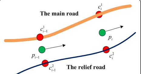
If the observation probability does not take into ac-count the topological connectivity among the road sec-tions of the potential points corresponding to the adjacent positioning points, mis-matching will occur. Figure6shows an example of mis-matching; if matching points are selected only by the observation probability value of potential matching point, the value of Nðc1iÞ is the maximum, then the matching point ofpiisc1i.
How-ever, if considering the previous and next point pi-1 and
pi + 1, then we find that the correct matching point is c2 i
of pi. Because if the matching point of piis c1i, the
ve-hicle must arrive onpi, starting from pi - 1, then return topi + 1, which is contrary to the previous rule 2.
2. Transition probability calculation
For the GPS location of two adjacent points pi - 1and
pi, their corresponding potential points are cs
i−1 and cti,
respectively, and the transition probability Vðcsi−1→ctiÞ from cs
i−1 to cti is defined as the coincidence degree
be-tween the real path and the shortest path. Consider the following conditions:
(a) When two potential pointscs
i−1andctiare located on
the same section or adjacent sections, the topological relation is determined, thenVðcs
i−1→ctiÞ ¼1.
(b) Transfer probability is mainly to analyze the topology fromcs
i−1tocti, then we should take the
distance fromcs
i−1tocti as the standard of
measurement. Therefore, transfer probabilityVðcs i−1
→ct
iÞis always in the range (0, 1].
Based on the above analysis, the transition probability is calculated as formula (10):
V c si−1→cti
1;in the same or adjacent sections dði−1;sÞ→ð Þi;t
3. Space analysis function
With the observation probability and transition prob-ability, the space analysis function can be defined as follows:
Fs csi−1→cti
¼N c ti V csi−1→cti ð11Þ
Formula (11) shows the possibility of a vehicle frompi - 1 moving to pi. Therefore, the distance between the posi-tioning point and the potential point, the instantaneous velocity of the positioning point, and the topology of the potential points are all utilized. Based on the space ana-lysis, for any two adjacent positioning pointspi - 1andpi, the potential points csi−1 and cti construct a series of weighted potential paths.
3.3.2 Analysis of time
In most cases, the proposed algorithm can identify the actual path from the potential paths. However, there are still some situations where we cannot effectively calcu-late the actual path only by the space analysis.
As shown in Fig.7, the thick line is a main road, the thin line next is an auxiliary road, we can get Fsðc1i−1→c1iÞ
¼ Fsðc2i−1→c2iÞ with the space analysis. However, if the
average speed frompi - 1topiis 80 km/h, considering the road speed limit, we can select the path fromc1
i−1 toc1i as
the matching path.
Given two GPS positioning pointspi-1 andpi, the cor-responding potential points are cs
i−1 andcti, respectively,
the shortest path from cs
i−1 to cti can be expressed as a
series of sectionse1,e2, …, ek, the average vehicle speed
in the shortest path can be expressed as:
vi−1→i¼
speed limit which can be used to measure the correl-ation between the average speed of the vehicle and the path speed limit. For the vector ðvi−1→i;vi−1→i;…;vi−1→iÞ
With the analysis of time and space, we can obtain the initial trajectory. However, if obtaining the accurate matching path results, we should process the result matching. We propose a segment partition method to accelerate the process of obtaining matching path.
3.4.1 Acquisition of matching path
With the analysis of time and space, it can generate a po-tential map GT(VT, ET) for the floating car trajectory T:
p1→p2→…→pn. VT is a set of potential points corre-sponding to all the GPS positioning points on the T.ETis a collection of edges, where each edge represents the shortest path between two adjacent GPS positioning points corre-sponding to the potential points. GT(VT, ET) is shown as Fig.8, where each node is related toNðcijÞand the weight of each edge is related toVðcs
i−1→ctiÞandFsðcsi−1→ctiÞ.
Combining formula (11) and formula (13), the space-time function can be defined as below:
F c si−1→cti ¼ Fs csi−1→cti
Ft csi−1→cti
ð14Þ
The potential matching path of trajectory T can be expressed asPc:cq11→c
q2
2 →…;→c qn
n. From the above
ana-lysis, we can find that the weight of each edge in the graph can be calculated with formula (14). The bigger the sum of the edge weights on the potential matching path is, the higher the possibility of being the matching result is. The total weight of each potential matching path is represented as FðpcÞ ¼Pni¼2Fðc
si−1
i−1→c si
iÞ. We can search for a path
from the potential matching paths to meet the maximum ofF(Pc), where the found path is the matching path of T. Formally, the best matching path Pof trajectory Tcan be expressed as:
P¼ arg maxpcF Pð Þc ; ∀Pc∈GTðVT;ETÞ ð15Þ
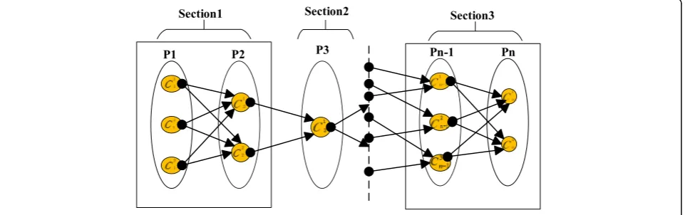
3.4.2 Sections division
all the potential points in the track T, we can obtain the best matching path. When the trajectoryTcontains a large number of positioning points or the need for online matching, the processing efficiency of the algorithm may be in difficulty in meeting the actual requirements. In order to improve the algorithm efficiency, our paper proposes a method of section dividing the potential matching path graphGT(VT, ET). After division, the matching path can be calculated in parallel for each section can calculate the matching path with the proposed methodology.
In the actual matching process, we find that the position-ing point correspondposition-ing to the potential point is unique sometimes by using the error region, direction angle, and other factors to filtering out the potential points. For ex-ample, as shown in Fig.9, whereP3has only one potential pointc1
3. In this case, the matching path ofGT(VT, ET) def-initely passc1
3. Thus, the map can be divided by a series of single potential point. And the topological relationship be-tween the potential points in the adjacent segment bound-ary is determined. After division, the potential matching path graph in Fig. 8will be divided into three sections as shown in Fig.9. The division of the potential matching path graph not only can reduce the execution time of the
algorithm, but also does not affect the accuracy of the map-matching algorithm.
3.5 Time complexity analysis of the proposed algorithm This section firstly analyzes the time complexity of the map-matching algorithm, and then optimizes the algo-rithm according to the analysis results.Nis used to indi-cate the number of positioning points in the trajectory
T,Mrepresents the number of road sections, andK rep-resents the maximum number of potential points of each positioning point.
The establishment of potential matching path graph
GT(VT, ET) requires the observation probability of each potential point. The weightETof each edge needs to cal-culate the transition probability and process time ana-lysis. After the establishment of GT(VT, ET), it is necessary to search for the critical path. The following is a detailed analysis for each calculation step:
1. The time complexity of observation probability: The maximum of all positioning points isnk, and the complexity of calculating the probability of each
Fig. 8Potential graphGT(VT, ET)
potential point isO(1), so the time complexity isO (nk).
2. The time complexity of transfer probability and time analysis: The number of the shortest paths that need to be computed in the potential matching path graph is(n-1)k2.The time complexity with Dijkstra algorithm to calculating the shortest path is O(v2), wherevis the number of segment endpoints in the road network (only counting once for repeating), thenv = m + 1, then the time complexity can be expressed asO((m + 1)2).Therefore, the time complexity of calculating the transition probability and process of time analysis isO(nk2m2).
3. The time complexity of matching path
computation: Because each edge of the potential matching path graph should be visited once, and the number of edges isnk2, then the time
complexity of the matching path computation isO (nk2).
Based on the above analysis, the time complexity of our proposed algorithm is O(nk2m2+ nk2+ nk). Consid-ering that the number of potential matching points for each GPS positioning point is a small positive integer, the time complexity of the matching algorithm can be approximated as O (nm2). The number mof urban road network is generally large, so the running time of the proposed algorithm would be a little big. In order to re-duce the running time of our proposed algorithm, we can optimize the computation of shortest path.
Firstly, considering the calculation process of Dijkstra algorithm,sis used to indicate the starting point,tis the end point, the array path represents the distance from the starting point to other points, and the set S stores the set of points in shortest path. The optimization steps are shown as follows:
1. Setting the initial value of the setSas empty, path[s] = 0, and the value of other points in the pathas positive infinity;
2. Searching for the point whose path value is the smallest one which is not in the setS, and then adding it to the setS, and use it to update the path value of the surrounding points;
3. Iftis not in the set S, repeat step (2) untiltis involved in the setS, and the process ends.
In the step (2), to search for the point whose path value is the smallest, normally the Dijkstra algorithm traverse the points not in theS, the complexity is O(v2). Here we can optimize the algorithm with the minimum heap algorithm, where the time complexity of the mini-mum heap algorithm is O(vlog v) to reduce the time complexity of the algorithm. Therefore, the total time
complexity of the proposed map-matching algorithm is reduced from O(nm2) to O(nmlogm). Besides, with the section division, the processing of difference sections can be done in parallel, which is helpful to improve the computational efficiency of the proposed algorithm.
4 Experiments simulation and results analysis 4.1 Experimental data
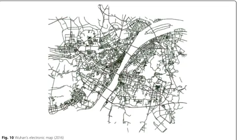
For the road network data, due to the limitations of the actual conditions, the experiment uses the electronic map of Wuhan in 2016, as shown in Fig. 10. The net-work data is extracted with Coordinate Extractor, a plug-in unit of MapInfo software. The Network’s parti-tion is divided by Grider Maker, which is also a plug-in unit of MapInfo software. The data is transferred and stored in the form of text files.
For the floating car data, data are acquired from a Wuhan company’s vehicle in 2016, where the GPS sam-pling time interval is 1 s. We select 20 groups of the floating vehicle trajectory data.
For matching result visualization, the map-matching results are output to the text file. Then we use the desk-top GIS system of MapInfo to display the matching re-sults in the electronic map.
4.2 Experimental simulation results
In order to measure the matching effect of the proposed map-matching algorithm for trajectory data of different sampling frequencies, we do the sample on each GPS tra-jectory data with the interval of 30, 60, 90, 120, 150, and 180 s, respectively, as the data to match. Then we pre-process these data and select the initial potential road and the potential points. The data in Table1present the short-est path information among part of potential points of the vehicle 1. The first line indicates the number of the short-est path of the potential points for vehicle 1. The second line indicates the shortest path information of two poten-tial points, where the first and the second number repre-sent the ID of potential points, For example, 00 means the ID 0 potential point corresponding to the ID 0 positioning point, the third number indicates the number of sections in the shortest path, the following numbers are the ID of the corresponding sections, and the last number repre-sents the length of the shortest path.
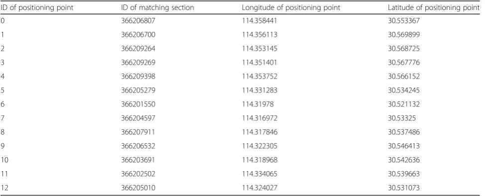
Then we process the analysis of the time and space and result matching to obtain the corresponding GPS matching path. Table 2 shows the matching results of the positioning points of vehicle 1. The first number represents the ID of the positioning point, the second number indicates the ID of matching section, and the third and the fourth numbers indicate the longitude and latitude corresponding to the positioning point.
Fig. 10Wuhan’s electronic map (2016)
Table 1Shortest path between some potential points
ID of potential points
ID of potential points
No. of sections
ID of the section
ID of the section
ID of the section
ID of the section
ID of the section
ID of the section
ID of the section
Length of the shortest path
00 10 5 366206807 366206805 366206803 366206801 366206700 1045
00 11 6 366206807 366206805 366206803 366206801 366200490 366200492 1494
01 10 7 366200485 366200487 366200488 366206489 366206490 366206689 366206700 1587
01 11 6 366200485 366200487 366200488 366206489 366200490 366200492 1248
02 10 6 366206808 366206807 366206805 366206803 366206801 366206700 1376
02 11 7 366206808 366206807 366206805 366206803 366206801 366200490 366200492 1794
10 20 5 366206700 366206701 366206703 366209263 366209264 985
11 20 6 366200492 366200495 366200496 366200497 366209263 366209264 1183
20 30 5 366209264 366209265 366209266 366209268 366209269 873
20 31 6 366209264 366209265 366209266 366209268 366209269 366209387 997
20 32 5 366209264 366209265 366209266 366209268 366209269 366209375 366209376 1034
30 40 6 366209269 366209387 366209388 366209389 366209397 366209398 1432
31 40 5 366209387 366209388 366209389 366209397 366209398 1147
32 40 6 366209376 366209377 366209378 366209379 366209380 366209397 366209398 1391
40 50 6 366209398 366209399 366209340 366209341 366204751 366204752 897
40 51 7 366209398 366209399 366209340 366209341 366204751 366204752 1268
are presented in the electronic map, as shown in Fig.11, where the black flag represents GPS positioning point of floating car, and blue pushpin represents the correspond-ing matchcorrespond-ing point.
4.3 Analysis of experimental results
The map-matching algorithm can be evaluated with two factors: running time and matching accuracy. The running time is the execution time of the algo-rithm in the actual environment. The matching accur-acy can be measured with two aspects: one is the correct matching ratio of positioning point, called AN; the other is the length accuracy ratio AL which is the ratio of the matching path length to the actual path length. And the calculation of AN and AL can be de-fined as follows:
AN ¼
Nr
N ð16Þ
AL¼
Lr
L ð17Þ
where Nr is the number of correct matching points,
N is the total number of positioning point, Lr is the matching path length, and L is the actual driving length. We compare our proposed algorithm with the global matching algorithm based on weak Fréchet dis-tance and the piecewise fuzzy matching algorithm over the running time and matching accuracy.
4.3.1 Measurement with running time
The running time of the algorithm is an important factor to measure whether the algorithm is practical when processing map matching for massive floating car data. In order to evaluate the running time of the
proposed algorithm, we compare the running time among the proposed algorithms, the global matching algorithm based on weak Fréchet distance [13], and the piecewise fuzzy matching algorithm [18]. The sampling time interval of the low-frequency floating car data is 120 s. Taking a different number of posi-tioning points for matching, the running time results of three algorithms are shown in Fig. 12. The experi-mental results show that the running time of the pro-posed algorithm is very close to the piecewise fuzzy matching algorithm, and it is better than the match-ing algorithm based on weak Fréchet distance. When the number of matching points increase, the compu-tation time of the matching algorithm based on weak Fréchet distance increases exponentially, but our pro-posed algorithm is almost stable. It indicates that the algorithm proposed in this paper is of good time efficiency.
Table 2Matching results of some positioning points
ID of positioning point ID of matching section Longitude of positioning point Latitude of positioning point
0 366206807 114.358441 30.553367
1 366206700 114.356113 30.569899
2 366209264 114.353145 30.568725
3 366209269 114.351401 30.567776
4 366209398 114.353752 30.566152
5 366205279 114.331283 30.534245
6 366201550 114.31978 30.521132
7 366204597 114.316972 30.53325
8 366207911 114.317846 30.537486
9 366206532 114.322305 30.546413
10 366203691 114.318968 30.542636
11 366202502 114.334065 30.539663
12 366205010 114.324027 30.531073
4.3.2 Matching accuracy
We take a sample of 20 sets of floating vehicle data with different sampling intervals and consider the average matching accuracy of these 20 sets of data as the final matching accuracy. We compare the matching accuracy among the proposed algorithms, the global matching algo-rithm based on weak Fréchet distance, and the piecewise fuzzy matching algorithm with the factor at different sam-pling intervals. We mainly compare the correct matching ratio of positioning pointAN, as shown in Fig.13, and the length accuracy ratioALas shown in Fig.14.
We can find that our proposed algorithm is superior to the other two algorithms in terms of accuracy. With the increase of the sampling time interval, the accuracy of three matching map-matching algorithms would de-crease then. When the sampling interval is 180 s, ANof the proposed algorithm is still as high as 83% andALis 81%. These results demonstrate that the proposed map-matching algorithm is able to make full use the low-frequency floating car data and obtain high match-ing accuracy with buildmatch-ing the optimized map-matchmatch-ing model combined with the network data.
5 Conclusions
In this paper, based on the analysis of low-frequency float-ing car data and the research of existfloat-ing map-matchfloat-ing al-gorithms, we propose an optimized map-matching algorithm based on matching path with low-frequency floating car data. The proposed algorithm takes full consid-eration of the factors such as vehicle distance, direction, speed, and road topology. Firstly, we preprocess the GPS data and road network data to determine the potential points and sections by constructing the error region. Then, we calculate the potential matching path graph with the analysis of time and space. Finally, we can obtain the matching result by parallel computing with sections div-ision methodology. With the contrast experiment in run-ning time and matching accuracy, we can find out when the sampling time of the floating car data is 120 s and the number of positioning point is 400, the running time of our proposed algorithm can be within 2 s, which is of high efficiency. Meanwhile, when the sampling interval is 180 s, the correct matching ratio of positioning point of the pro-posed algorithm is up to 83%, and the length matching ac-curacy ratio is up to 81%, which is more accurate than other algorithms.
With the construction of the city in the future, the road will be more and more three-dimensional. In the future, the map-matching algorithm will expand to the three-dimensional map matching.
Abbreviations
ITS:Intelligent Transportation System; RPF: Road reduction filter; AOE: Activity on edge
Funding
The funding of the authors can support the publication of the manuscript. This work was supported by the National Natural Science Fund of China under grant 61502185 and the Fundamental Research Funds for the Central Universities (No: 2017KFYXJJ071).
Availability of data and materials
The data and related materials will be available when requiring. Fig. 12Running time of different algorithms
Fig. 13Results ofANat various intervals
Authors’contributions
The authors’contribution is to propose a map-matching algorithm with the low-frequency floating car data, which can improve the accuracy and efficiency of map matching to select the correct matching path rapidly. All authors read and approved the final manuscript.
Authors’information
Ling Yuan is currently an associate professor in the School of Computer Science and Technology, HUST, Wuhan, P.R. China. She received her Ph.D. degree in the Department of Computer Science from National University of Singapore in 2008. She received her B.S degree and M.S. degree in computer science from Wuhan University, Wuhan, China, in 1997 and 2002, respectively. Her research interest includes data processing and software engineering.
Dan Li is currently an associate professor in School of Computer Science and Technology, HUST, Wuhan, P.R. China. She received the B.E. and M.S. degrees in mechanical design, manufacturing and automation from Huazhong University of Science and Technology (HUST), Wuhan, China, in 1998 and 2002, respectively, and the Ph.D. degree in computer science from HUST in 2008. Her research spans computer graphics, multimedia, and intelligence. Song Hu is pursuing his Master degree in computer science and technology at the School of Computer Science and Technology, Huazhong University of Science and Technology, HUST, Wuhan, P.R. China. He received the Bachelor’s degree in the College of software from Xidian University, Xian, China, in 2016. His research interests include computer graphics and computer vision.
Competing interests
The authors declare that they have no competing interests.
Publisher’s Note
Springer Nature remains neutral with regard to jurisdictional claims in published maps and institutional affiliations.
Received: 2 January 2018 Accepted: 25 May 2018
References
1. Editorial Department of Chinese Journal of highway, Summary of academic research on traffic engineering in China 2016. China J. Highw. Transp. (06), 1–161 (2016)
2. Z Na, Y Jiabin, X Han, Overview of intelligent transportation system. Comput. Sci. (11), 7–11+45 (2014)
3. H Libin, The survey of city intelligent traffic system’s construction at home and abroad. City Bridg. Flood Control (05), 40–45+8 (2016)
4. K Zheng, D Zhu, Progress in the application of floating car technology. Mod. Electron. Technol. (11), 156–160 (2016)
5. H Abbott, D Powell, Land-vehicle navigation using GPS. Proc. IEEE87(1), 145–162 (1999)
6. H Cheng, Z Su, N Xiong, Y Xiao. Energy-efficient Node Scheduling Algorithms for Wireless Sensor Networks, Information Sciences,2016,329 (2): 461–477.
7. H Cheng, N Xiong, A V. Vasilakos. L T Yang, G Chen, et. al, Nodes Organization for Channel Assignment with Topology Preservation in Multi-radio Wireless Mesh Networks, Ad Hoc Networks,2012,10 (5): 760-773. 8. S Dihua, Z Xingxia, Z Zhiliang, Map matching technology and its application
in intelligent transportation system. Comput. Eng. App. (20), 225–228 (2005) 9. D Bernstein, A Kornhauser,An Introduction to Map Matching for Personal
Navigation Assistants(USA, New Jersey TIDE Center, 1996)
10. G Taylor, G Blewitt, D Steup, S Corbett, A Car, Road reduction filtering for GPS-GIS navigation. Trans. GIS5(3), 193–207 (2001)
11. JS Greenfield, inProceedings of the 81st Annual Meeting of the Transportation Research Board, January, Washington D.C.. Matching GPS Observations to Locations on a Digital Map (2002), pp. 2561–2573
12. H Alt, A Efrat, G Rote, C Wenk, Matching planar maps. J. Algorithm.49, 262– 283 (2003)
13. S Brakatsoulas, D Pfoser, R Salas, et al., inProceedings of the 31st VLDB Conference. On map-matching vehicle tracking data (IEEE, Trondheim, 2005), pp. 853–864
14. P Fei, Map matching algorithm for integrated navigation system based on cost function. J. Beihang Univ.28(3), 261–264 (2002)
15. J Gao, S Juan, S Xiaolin, Study on the method of navigation road map matching based on the filter. Eng. Surv. (11), 77–79 (2009)
16. S Kim, JH Kim, Adaptive fuzzy-network based C-measure map-matching algorithm for car navigation system. IEEE Trans. Ind. Electron.48(2), 432–441 (2001)
17. W Xiaomeng, C Tianhe, et al., A map matching method for massive floating car data. J. Earth Inf. Sci.17(10), 1143–1150 (2015)
18. Y Enjian, Real time map matching algorithm based on low frequency floating car data. J. Beijing Univ. Technol.39(6), 909–913 (2013) 19. J Shen, Z Tinggang, Z Hongtao, A map matching algorithm for low
frequency floating vehicle based on improved AOE neural network. J. Southwest Jiao Tong Univ.50(3), 497–503 (2015)
20. V Walter, D Fritsch, Matching spatial data sets: A Statical approach. Int. J. Geogr. Inf. Syst.13(5), 445–473 (1999)