Simultaneous Principal Component Extraction with Application to Adaptive Blind Multiuser Detection

(1)

Simultaneous Principal-Component Extraction

with Application to Adaptive Blind

Multiuser Detection

Deniz Erdogmus

Computational NeuroEngineering Laboratory, Electrical and Computer Engineering Department, University of Florida, NEB 454, Gainesville, FL 32611, USA

Email: [email protected]

Yadunandana N. Rao

Kenneth E. Hild II

Jose C. Principe

Received 31 January 2002 and in revised form 30 July 2002

SIPEX-G is a fast-converging, robust, gradient-based PCA algorithm that has been recently proposed by the authors. Its superior performance in synthetic and real data compared with its benchmark counterparts makes it a viable alternative in applications where subspace methods are employed. Blind multiuser detection is one such area, where subspace methods, recently developed by researchers, have proven eﬀective. In this paper, the SIPEX-G algorithm is presented in detail, convergence proofs are derived, and the performance is demonstrated in standard subspace problems. These subspace problems include direction of arrival estimation for incoming signals impinging on a linear array of sensors, nonstationary random process subspace tracking, and adaptive blind multiuser detection.

Keywords and phrases:principal-component analysis, multiuser detection, SIPEX.

1. INTRODUCTION

Principal-component analysis (PCA) is a fundamental statis-tical technique that has established its significance in signal processing through numerous successful applications includ-ing, but not limited to, feature extraction, signal estimation, detection, speech separation, linear discriminant analysis, di-rection of arrival estimation, and subspace filtering [1, 2, 3, 4, 5]. There are many algorithms that have been proposed for solving the PCA problem both oﬀ-line and on-line; specifi-cally, Oja’s rule [6] ignited an interest among researchers for on-line PCA algorithms. Sanger’s rule [7], Rubner-Tavan al-gorithm [8, 9], and APEX [2] are immediate extensions to Oja’s update rule. These conventional topologies and their

(2)

There are also well-known fast-converging rules for PCA, like the natural power method and the fixed-point rule [5, 10]. However, they still use the deflation scheme to determine the intermediate eigenvectors after the principal component has converged, which prevents the algorithms from converg-ing simultaneously to all the components. Xu’s LMSER algo-rithm uses subspace techniques and a diagonal amplification matrix to extract the principal components simultaneously [11]. Although LMSER introduces a great improvement over the traditional methods in terms of speed and accuracy, it does not constrain the search space for the PCA weight ma-trix to the set of orthonormal matrices, and therefore, must search the entire space when trying to orthonormalize the estimated eigenvectors. Our SIPEX-G algorithm (simulta-neous principal-component extraction—gradient-based ap-proach), on the other hand, employs Givens rotations as an orthonormal parameterization of the PCA weight matrix and uses a robust and consistent estimate of the output variances (based on the input vector’s covariance estimate) in order to converge quickly and accurately to the eigenvectors of the un-derlying covariance matrix [12, 13].

There has been considerable interest and recent research in the field of multiuser detection [14], specifically,adaptive multiuser detection [15, 16, 17, 18, 19, 20, 21, 22]. Within this framework, subspace methods for code division multiple access (CDMA) channel estimation and for multiuser detec-tion have also been investigated [18, 19, 20, 21, 22, 23]. Blind multiuser detection is useful for inter symbol interference (ISI) suppression in CDMA uplinks as well as in downlinks, where the mobile receiver has knowledge of its own spread-ing sequence only. The gain in the uplink is relatively small as the base stations usually have access to all the spreading se-quences in their cells. Group-blind methods may, in this case, be helpful in decreasing the interference from the users with unknown spreading sequences if there are any [19]. As in any subspace-based approach, the performance of the PCA algo-rithm, that is employed, has a considerable impact on the overall success of the solution.

In this paper, we present a complete derivation of the SIPEX-G algorithm and provide a proof demonstrating that the combination of the proposed cost function and topology form a system in which all of the stationary points are solu-tions to the PCA problem. We also demonstrate the perfor-mance of SIPEX-G on a number of signal processing appli-cations including nonstationary subspace tracking, direction of arrival estimation, and blind multiuser detection.

2. THE COST FUNCTION, THE TOPOLOGY, AND THE SIPEX-G ALGORITHM

It is well known that the directions of the principal compo-nents are given by the eigenvectors of the covariance ma-trix of the input data, ordered according to their corre-sponding eigenvalues in descending order of magnitude [24]. Thus, PCA is nothing more than a coordinate transformation on the data, where, in the new coordinate system, the axes are aligned with the directions of maximal variation. This

immediately points out that the search for the weights of a principal component network can be restricted to the set of orthonormal matrices since every orthonormal transfor-mation corresponds to an axis-rotation in the input vec-tor space. Consider the principal component network with

y = Rx, wherex ∈ Rn×1 _and_y _∈ _Rn×1_{are the input and}

output vectors, respectively, andR ∈D⊂Rn×n_{is the PCA}

weight matrix which is restricted to the subsetDof orthonor-mal matrices. The cost function in (1) could be maximized (or minimized) in order to determine the principal (or mi-nor) components of the input data whose covariance matrix is given byΣx. Considering the case where (1) is maximized, the scalar gainsγsare chosen in descending order (ascending

if (1) is minimized) such thatγ1 > γ2 > · · · > γn−1 > 0.

Thus, the cost function is just the weighted sum of the first (n−1) output variances. In the subsequent discussions, we assume that the input data xis zero-mean, without loss of generality,

J=

n−1

s=1

γsVar

ys

. (1)

The utility of this cost function, when used together with the proposed orthonormal network topology, is established by the following theorem. This theorem states that when our objective is to determine the complete set of principal components, any stationary point of this cost-topology pair yields the desired solution although they might not be in de-scending or ade-scending order. However, as we will see in the sequel, if necessary, this ordering could be achieved at no ad-ditional computational cost since the algorithm already pro-vides everything necessary to determine the ordering of the eigenvectors.

Theorem 1. For the constrained PCA network whereRis an orthonormal matrix, the function J in (1) has a stationary point if and only if all the rows ofR consist of all the eigen-vectors of Σx.

Proof. See the appendix.

Corollary 1. There are totallyn!stationary points ofJof which (n−1)!are local maxima,(n−1)!are local minima, and(n−

2)(n−1)!are saddle points.

Proof. This follows easily from the ideas in the proof of Theorem 1. The (n−1)! local maxima correspond to all pos-sible permutations of the (n−1) maximum eigenvectors be-ing placed in the first (n−1) rows ofR. Similarly, the (n−1)! local minima correspond to all possible permutations of the (n−1) minimum eigenvectors being placed in the last (n−1) rows ofR. All other permutations of the eigenvectors inR, which amount to (n−2)(n−1)!, are saddle points.

(3)

the rows of the PCA weight matrixRwill give us the desired eigenvectors of the input covariance matrix. It is also possible to include in the cost function given in (1) only the variances of the firstmoutputs. Global maximization of this new cost function will result in the convergence of the firstmrows of the rotation matrix to the firstmprincipal components. Oth-erwise, if the summation in (1) does not go up ton−1 due to Corollary 1, the firstmrows ofRwill correspond to some collection ofmeigenvectors depending on which local max-imum is attained. The gainsγicome into play at this point.

By careful assignment of the scale factors to the outputs, it is possible to force the solution towards the global maximum. This procedure, however, is beyond the scope of this paper. In the following, we will concentrate only on the case where all the eigenvectors are to be determined and their order is not important.

Now, we focus on finding a suitable parameterization for the orthonormal PCA matrix. Every orthonormal ma-trix can be considered a rotation mama-trix, thus, they can be parameterized in terms of Givens rotation angles, each of which define a rotation in a single (two-dimensional) plane of the high-dimensional vector space. Then, these individ-ual rotations can be cascaded together to span the whole set of orthonormal matrices. Every rotation matrix has a unique set of Givens rotation angles that characterize it. In n-dimensions, a Givens rotation matrix in the plane, formed by the pth andqth axes, is denoted by Rpq _{and is given by}

an identity matrix whose four entries at the intersection of pth andqth rows with pth andqth columns are modified as follows: the (p, p)th and (q, q)th entries are cosθpq, and the

(p, q)th and (q, p)th entries are−sinθpqand sinθpq,

respec-tively [5]. The complete rotation matrix is then formed from these sparse matrices according to

R=

n−1

p=1

n

q=p+1

Rpq. (2)

The multiplication order can be always from the left or always from the right. It is not crucial to the generality of this formula as long as the same order is maintained when tak-ing the derivative of the matrix with respect to each rotation angle. To summarize, our objective is to solve the following unconstrained optimization problem parameterized in terms of the Givens rotation angles.

Problem1. Letθpq,p=1, . . . , n−1,q= p+ 1, . . . , nbe the

Givens rotation angles that constitute our parameter vector Θ. The cost function is explicitly given by

J(Θ)=

n−1

s=1

γsVar

ys

=

n−1

s=1

γs n

i=1

n

j=1

RsiRs jΣx,i j, (3)

where R_{s j} is the (s, j)th entry of the orthonormal matrix

R, which is constructed using the Givens rotation angles as shown in (2), andΣx,i jis the (i, j)th entry of the input

covari-ance matrix. Since all stationary points of this cost function

yield the desired eigenvectors, minimization or maximiza-tion of (3) may be employed during optimizamaximiza-tion.

The Givens angles provide a suitable representation for the PCA weight matrix in that it guarantees that the search is limited to the set of orthonormal matrices. The cost function, ideally, provides an eﬀective means of forcing the weight ma-trix towards the desired eigenvectors. In practice, however, we neither have access to the actual input covariance ma-trix nor to a parametric expression of the output variances in terms of the Givens angles. Therefore, the proposed al-gorithm utilizes a robust and consistent nonparametric esti-mator for the cost function. To this end, the following well-known recursive sample-estimate for the input covariance matrix is employed:

ˆ

Σx(k)=αΣˆx(k−1) + (1−α)x(k)xT(k). (4) In this expression, the notation ˆΣx(k) is used to distinguish the sample-estimate of the input covariance matrix at timek from its true valueΣx. The adjustable parameterα∈[0,1) is the forgetting factor andx(k) is thekth input vector sample. Note that the recursion in (4) can be used for both wide sense stationary (WSS) and nonstationary input signals. If the in-put is known to be WSS, the following recursive estimator, which is unbiased and consistent, may be utilized:

ˆ

Σx(k)=k− 1

k Σˆx(k−1) + 1 kx(k)x

T₍_k₎_. ₍₅₎

Using this estimate for the covariance matrix for WSS data will improve the performance of the estimate, and therefore, the algorithm. In both recursions, the covariance estimate

ˆ

Σx(k) can be initialized using the firstN > nsamples using the unbiased sample estimate (for WSS data) of the covari-ance matrix (recall that we assumedxis zero mean)

ˆ Σx(0)=

1 N

N

l=1

x(l)xT(l). (6)

The approach presented above, which uses the input co-variance matrix estimate and the current values of the PCA weight matrix to estimate the output variances, assures a ro-bust estimate of the cost function. More importantly, the es-timate of the gradient of this cost function is robust which leads to a smooth and fast convergence to the desired so-lution. If, instead, the output variances are estimated di-rectly from the output samples using either a batch of out-put values or only the most recent outout-put value, as in the traditional approach to PCA estimation, we would risk los-ing these advantageous properties; in fact, simulations with diﬀerent schemes in estimating the output variances have demonstrated that the proposed approach provides the best convergence results both in terms of convergence speed and accuracy.

(4)

approach. We know from many applications in signal pro-cessing and communications that gradient-based algorithms are successful in on-line adaptation schemes because of their ability to handle nonstationary signals as well as time-varying models. Below, we briefly describe the SIPEX-G al-gorithm which uses gradient ascent optimization.

Algorithm 1. Simultaneous principal-component extraction using the gradient approach (SIPEX-G)

(1) initialize Givens angles (randomly or to all zeros so that the initial rotation matrix is the identity matrix); (2) initialize the estimate of the input covariance matrix

us-ing(6);

(3) for non-WSS signals and/or time-varying environments, update the covariance estimate using(4). If the input is WSS and the environment is time-invariant use(5); (4) calculate the gradient of the cost function in(3)with

re-spect to the Givens angles (substituting the input covari-ance with its most current sample-estimate). The gradi-ent is

∂J ∂θpq =

n−1

s=1

n

i=1

n

j=1

Rsi∂

Rs j

∂θpq +

∂Rsi

∂θpqRs j

ˆ

Σx,i j; (7)

(5) update the Givens angles using gradient ascent/descent

Θ(k+ 1)=Θ(k) +η_∂Θ∂J , (8)

whereηis an adjustable step size;

(6) go back to step 3 and continue as long as input samples arrive.

A key concern in many adaptive algorithms is the com-putational complexity. It is clear that if the multiplications in (2) are performed from the left, the first output is only af-fected from the Givens angles with indicesθ1q,q =2, . . . , n,

the second is aﬀected by all the anglesθ1q,q =1, . . . , nand

θ2q,q =3, . . . , n, and so on. Thus, if we wish to extract the

firstmprincipal components, we only need to adapt the an-gles θi j,i = 1, . . . , m, j = i+ 1, . . . , n, which makes a total

ofmn−m(m+ 1)/2 parameters, which is less than themn parameters required in many PCA algorithms. The trade-oﬀ is that the sin or cos of all these parameters must be eval-uated, which increasescomputational complexity. This could be somewhat alleviated, however, by means of a lookup table. In addition, the necessary matrix and vector multiplications in the algorithm must be performed at each iteration, which amount toO(mn2_{) operations. Specifically, the gradient in}

(7) has a complexity ofO(n3_{), which is more than the}

min-imum computational complexity that a fully stochastic PCA algorithm can achieve, which is O(n2_{). Although SIPEX-G}

has a higher complexity, it has superior convergence proper-ties due to the fact that the search is restricted to the set of orthonormal matrices only; this will also guarantee simulta-neous convergence of all principal components.

Another crucial issue in all adaptive learning algorithms is stability. In gradient-based algorithms, the stability and

speed of convergence are coupled and are controlled by the step size. For initial fast convergence, we usually require a large step size; however, increasing the step size without bound leads to algorithmic instability. We address the prob-lem of selecting a stable step size for SIPEX-G when max-imizing the cost function in (3) using (8) in the following theorem.

Theorem 2. The following upper bound on the step size of SIPEX-G guarantees stable convergence to the global maximum of (3)using the steepest ascent optimization approach. Never-theless, larger step sizes might be stable as well:

η≤n−1 1

p=1

n q=p+1

−γpλp−γqλq+γpλq+γqλp

, (9)

where λj is the jth largest eigenvalue of the input covariance

matrix.

Proof. See the appendix.

We have previously studied the performance of the SIPEX-G algorithm and how it compares to several bench-mark algorithms, including Sanger’s rule [7], APEX [2], and LMSER [11], in two previous publications [12, 13]. Exten-sive Monte Carlo simulations, performed for this purpose, demonstrated the superior performance of SIPEX-G both in terms of convergence speed and final accuracy in esti-mating the eigenvectors of the input covariance matrix. The case studies for these simulations included synthetic Gaus-sian data, recorded violin time-series analysis, and adaptive filter training (Wiener solution) using PCA. From these sim-ulations, the LMSER algorithm proved to be the strongest competitor. For this reason, the proposed algorithm is only compared to LMSER in the simulations that follow.

3. NONSTATIONARY SUBSPACE TRACKING WITH SIPEX-G AND LMSER

In order to demonstrate the superior speed and accuracy of SIPEX-G in subspace tracking, we present in this section a synthetic nonstationary scenario where three colored ran-dom time series, having varying covariance matrices were concatenated. The composite time series is then presented to SIPEX-G, which used a step size of 0.002 and a forgetting factor of 0.999, to estimate the three principal components. The scalar gains of SIPEX-G were set to [1, 2, 3]. As expected, the speed of convergence and accuracy depend mainly on the forgetting factor.

(5)

18000 16000 14000 12000 10000 8000 6000 4000 2000 0

Samples 0

5 10 15 20 25 30 35 40

Ei

gen

va

lu

e

First-numerical Second-numerical Third-numerical

Figure1: SIPEX-G tracking the eigenvalues of the covariance

ma-trix of a 3-dimensional nonstationary random process. The refer-ence eigenvalues indicated by (∗) on the plot are determined using the MATLABeigfunction.

segments. Clearly, SIPEX-G is able to track the changes in the subspace structure of the input signal fast and with ac-ceptable accuracy.

As a second result, we present a comparison of the per-formances of SIPEX-G and LMSER on the same experimen-tal setup. The same composite time series, having varying eigenspreads, is now embedded in a 4-dimensional space. We use both SIPEX-G and LMSER to estimate all four princi-pal components. In the tracking results presented in Figure 2, SIPEX-G uses a constant step size of 0.005 and LMSER uses the maximum step size of 0.001 to ensure stability in all sta-tionary regions. The scalar gains of both algorithms were again set to [1, 2, 3, 4]. The angles between the four estimated and actual eigenvectors of the nonstationary covariance ma-trix are shown (in degrees) to reduce to the desired value of zero, almost accurately for SIPEX-G, in particular. The sud-den jumps in the angles within the third regime are due to the switching between reference eigenvectors along the gradient trajectory; these are not of much concern.

The convergence results of SIPEX presented in Figure 1 exhibits the expected transition behavior after each abrupt change in the input covariance matrix. In Figure 2, how-ever, the first abrupt changeseemsto be smoothly absorbed by SIPEX. On the other hand, LMSER, which was slow to converge during the first regime, converges to the solu-tion rapidly after the first abrupt change. These observasolu-tions should not be generalized. Notice that SIPEX still experiences the transition period after the second abrupt change, and LMSER is still slow to converge. The behavior of these two algorithms during the first transition can be explained by the fact that the first abrupt change does not instigate a large de-viation in the eigenvectors and the state of both algorithms are, therefore, already close to their optimal solutions for the

18000 16000 14000 12000 10000 8000 6000 4000 2000 0

Samples 0

50 100 150 200 250 300

An

gl

e

in

d

eg

re

es

SIPEX tracking

∗_Indicates change of covariance

(a)

18000 16000 14000 12000 10000 8000 6000 4000 2000 0

Samples 0

50 100 150 200 250 300

An

gl

e

in

d

eg

re

es

LMSER tracking

∗_Indicates change of covariance

(b)

Figure 2: Comparison of (a) SIPEX-G and (b) LMSER tracking

the eigenvectors of the nonstationary covariance matrix of a 4-dimensional random process. The angle between estimated and ac-tual eigenvectors are presented in degrees. The reference eigenvec-tors are evaluated using the MATLABeigfunction. Sudden changes are introduced in the covariance matrix at times of 5000 and 10000 samples, which are indicated by asterisks in the plot.

second regime. Since SIPEX is faster to converge in general, it acts quickly and recovers from the transition fast (still there is a short transition phase; notice the smallbumpin the an-gle errors immediately following the change). LMSER seems to converge faster because the change results in an optimal solution that is closer to the current state of this algorithm compared to the optimal solution of the first regime; there-fore, LMSER speeds up.

These two experimental results, obtained using nonsta-tionary covariance matrices, demonstrate the fast and accu-rate convergence of SIPEX-G as well as its ability to track changes in a nonstationary environment. Figure 1 demon-strates that the eigenvalues of the changing covariance matrix are tracked, and Figure 2 demonstrates that the eigenvectors (which are more crucial to the multiuser detection applica-tion) are also tracked.

4. APPLICATION OF SIPEX-G TO COMPLEX-VALUED SIGNALS

(6)

employed. Another application is the direction of arrival es-timation; this problem deals with the estimation of multiple source directions when signals from these sources impinge on an array of antennas. Once the source directions are esti-mated, this information could be used to improve the signal quality for a specific user by reorienting the antennas or by algorithmically processing the signal.

Direction of arrival estimation

Subspace-based methods for estimating the direction of ar-rival (DOA) of signals impinging on an array of sensors have been researched extensively. State-space method [25], ESPRIT [26], MUSIC (multiple signal classification) [27], and Min-Norm [28] are examples of these approaches to the DOA problem. These methods all require the eigendecom-position of the covariance matrix of the signal, yet the al-ternative SWEDE [29] achieves subspace estimation without eigendecomposition. In this section, we focus on the MU-SIC algorithm, which basically uses Sanger’s rule [7] for the eigendecomposition task. We then replace Sanger’s rule with our SIPEX-G algorithm.

The DOA problem is formulated as follows. A linear array ofnsensors receives a mixture of msource signals plus an additive complex Gaussian noise whose variance is smaller than those of the signals,

x(k)=D(Φ)s(k) +v(k), (10)

where D(Φ) = d(ϕ1) · · · d(ϕm) is then×m steering

matrix withΦdenoting the vector of direction angles of the sources [27, 29]. The random vectorsx(k),s(k), andv(k) are n×1,m×1, andn×1 complex Gaussian distributed random vectors, respectively. Using this formulation, the covariance matrix ofx, the received signal vector at the sensors, can be expressed as

Σx=E

x(k)xH(k) =D(Φ)ΣsD(Φ)H+σ2I (11) assuming uncorrelated, equal-power noise at each sensor. In order to solve the complex eigenvectors ofΣx, we define

Σc₌

ReΣx −Im

Σx ImΣx Re

Σx

, ec₌

Reex Imex

, (12)

where Σc _{is a real matrix that is twice the number of rows}

and columns ofΣx, andecis a single eigenvector ofΣc corre-sponding to the eigenvectorex of Σx. The matrixΣccan be computed from the samples by

Σc₌_E_xc_xcT _, _xc₌

Re[x] −Im[x] Im[x] Re[x]

. (13)

When the number of sources is known, the task of DOA esti-mation reduces to finding then-mminor components of the covariance matrixΣxand determining themminima of the cost function

f(φ)=d(φ)H_W

vWvH

d(φ), (14)

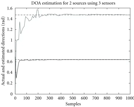
1000 900 800 700 600 500 400 300 200 100 0

Samples 0

0.2 0.4 0.6 0.8 1 1.2 1.4 1.6

A

ctual

and

estimat

ed

dir

ections

(r

ad)

DOA estimation for 2 sources using 3 sensors

Figure3: Actual and estimated DOA for a 2-source 3-sensor case

with 20 dB SNR.

where Wv =

e_m+1 · · · en is the matrix formed by the

eigenvectors corresponding to the minor components. This is called the MUSIC algorithm for DOA estimation.

When we apply SIPEX-G with gains [1, 2, 3, 4, 5, 6] and step size 0.01 to the MUSIC algorithm outlined above for a 2-source 3-sensor case with an signal-to-noise ratio (SNR) of approximately 20 dB, we obtain the result presented in Figure 3. The PCA problem for this case study is 2n=6 di-mensional, and there are three eigenvalues, each of multiplic-ity two. In this simulation, the two minima of the function in (14) are determined by simply evaluating it over theφvalues in the interval [0, π].

Notice that, in order to apply the SIPEX-G algorithm, which was originally designed to extract real-valued eigen-vectors from a real-valued symmetric covariance matrix, to the complex-valued DOA problem, we have introduced the modifications outlined in (12) and (13). As a direct conse-quence of the additional degrees of freedom introduced by the imaginary parts of the data, each n-dimensional PCA problem in the complex domain becomes a 2n-dimensional problem in real values.

5. APPLICATION OF SIPEX-G TO BLIND MULTIUSER DETECTION

(7)

al. [19, 20]. Therefore, we do not consider the asynchronous case explicitly here.

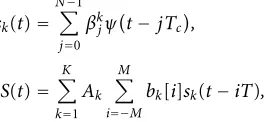
We consider a baseband digital direct sequence CDMA network ofKusers. In the synchronous scheme, the received signal can be expressed asr(t)=S(t) +σn(t), wheren(t) is zero-mean unit-variance white Gaussian noise andS(t) is the superposition of the data signals of theKusers active in the system. We have

sk(t)= N−1

j=0

βkjψ

t−jTc

,

S(t)=

K

k=1

Ak M

i=−M

bk[i]sk(t−iT),

(15)

whereψ(t) is the chip waveform with support [0, Tc],bk[i] is

the i.i.d. equiprobable bit sequence of userk,Akis the

chan-nel gain for userk’s signal,βkj,j=0, . . . , N−1 is the signature

sequence (also known as the spreading sequence) for userk, andTis the bit duration and, by definition, it isT=NTc. If

we collect the signature sequence of thekth user in a vector

sk and normalize its norm to unity, and if we collect all the

samples (at fractions of the chip durationTc) during a time

interval ofTseconds (called the bit duration) in a vectorr, we get the following vector equation:

r=

K

k=1

Akbksk+σn, (16)

wheresk=

β0k · · · βkN−1

T

/√Nandnis a zero-mean ran-dom process having an identity (IN) covariance matrix. We

assume that the signature waveform vectors of diﬀerent users are linearly independent. DefiningA=diag(A2

1, . . . , A2K) and

S=s1 · · · sK , the covariance matrix of the random

vec-torris found to be

Σr=E

r·rT =SAST+σ2_I

N. (17)

The covariance matrix can be decomposed into its signal and noise subspaces as

Σr=UΛUT=

Us Un Λs

0 0 Λn

UT

s

UT

n

, (18)

where the eigenvalues and their corresponding eigenvectors are in descending order (notice that the intrinsic assumption in this approach is that the noise power is smaller than the smallest signal power). The signal subspace isK-dimensional in theN-dimensional complete space (assuming we get one sample for every chip duration). Ideally, the signal-space eigenvectors of the covariance matrix are the spreading se-quences of all the users, as is evident from [17]. In the blind detection scheme, we assume that the receiver has knowl-edge of the signature waveform of only one user. For thekth user, it can be shown that the minimum mean square error (MMSE) receiver is given by [22]

ˆ

bk[i]=wT(k)r[i], (19)

wherer[i] is the received signal vector of dimensionNat the ith symbol duration [22] and

w(k)= UsΛs−1UTssk

sT_kUsΛ−s1UTssk .

(20)

The task is to estimate theK-dimensional signal subspace

Us. In the simulations, we use the SIPEX-G algorithm on the samplesr[i] of the received signal vector. For the spreading sequences, we utilize BPSK random signature sequences of lengthN=7. There are three active users in the system and each transmits a 60000-length BPSK symbol sequence (syn-chronously). The step size for SIPEX-G is held constant at 0.002. In order to show the convergence of the detectors to their optimal values, we use two measures: the angle between the estimated and optimal detector coeﬃcients (evaluated by taking the arccos of the direction cosine between these two vectors), and the signal-to-interference ratio (SIR) between the desired user’s signal and the combined multiple access interference (MAI) and channel noise defined in [16]. The SIR for thejth user is defined as

SIRj=

A2j

wT_jsj

2

N0wj

2

+Kk=1

k=jA

2

k

wT_jsk

2. (21)

First, we show the convergence of the receivers com-puted using the estimated eigendecomposition of the signal covariance matrix to their optimal values (evaluated using the MATLABeig function). Notice in Figure 4a that the re-ceivers of all users converge to their corresponding optimal values and in Figure 4b, the maximum theoretical SIR possi-ble for each user is achieved in less than 2000 samples. Only one update was performed for each sample; however, if time and computational bandwidth permits, multiple updates per sample could be performed to allow convergence to the solu-tion with an even smaller number of symbols.

Finally, we depict the bit error rate (BER) versus SNR plots for all three users in the above adaptive blind multiuser detection scenario, where SIPEX-G is used to determine the optimal blind MMSE receivers for the users. The BER curves shown in Figure 5 exhibit perfect match with the theoreti-cal expectations, which are superimposed on each plot. In Figure 5a, the numerically estimated BER is smaller than its theoretical expectation at large SNR values because of the limited number of symbols to estimate such small probabili-ties.

(8)

2 1.5

1 0.5

0

×104 Number of bits

0 50 100 150 200 250

An

gl

e

in

d

eg

re

es

Angle between the optimal and estimated receiver for three users

User 1 User 2 User 3

(a)

2 1.5

1 0.5

0 8.5

9 9.5

SIR for all users

User 1

2 1.5

1 0.5

0 0 5 10

User 2

2 1.5

1 0.5

0 −10

0 10

User 3

×104 Number of bits

Estimated

Theoretical maximum (b)

Figure4: SIPEX-G in blind multiuser detection. (a) The angle (in

degrees) between the estimated and true optimal receiver gain vec-tors. (b) The theoretical maximum and actual SIR performances obtained by the estimated optimal detectors for all users versus the number of symbols.

6. CONCLUSIONS

PCA is an important statistical methodology that finds appli-cations in the solutions of many important practical prob-lems of engineering including signal processing and com-munication. In this paper, we have presented a new, fast,

6 4 2 0 −2 −4 −6 −8 −10 −12

SNR in dB 10−5

10−4 10−3 10−2 10−1 100

P

robabilit

y

o

f

er

ror

BER for user 1

Theoretical Estimated

(a)

6 4 2 0 −2 −4 −6 −8 −10 −12

SNR in dB 10−2

10−1 100

P

robabilit

y

o

f

er

ror

BER for user 2

(b)

6 4 2 0 −2 −4 −6 −8 −10 −12

SNR in dB 10−2

10−1 100

P

robabilit

y

o

f

er

ror

BER for user 3

(c)

Figure5: The estimated 60000 symbols and theoretical (∗) BER

(9)

and robust PCA algorithm, where the topology is based on Givens rotations to guarantee orthonormality of the esti-mated PCA weight matrix at each iteration step. The cost function is parameterized in terms of the weight matrix and the input covariance matrix, which is estimated recursively from the input samples, to guarantee robustness and accu-racy of the final eigenvector estimates.

We have previously established the superior performance of SIPEX-G by comparing with benchmark PCA algorithms such as Sanger’s rule, APEX, and LMSER in a variety of prob-lems including both synthetic and real data. In this paper, we have demonstrated the superiority of SIPEX-G over LMSER in subspace tracking when the covariance matrix of the ran-dom process is nonstationary. In addition, we have demon-strated the application of SIPEX-G to complex-valued PCA through the use of a direction of arrival estimation example. The SIPEX-G algorithm was also tested on the blind mul-tiuser detection problem in DS-CDMA communication sys-tems using the synchronous signal model with a subspace ap-proach. The simulation results indicated that SIPEX-G was successful in determining the optimal blind MMSE receivers accurately using a very small number of samples. In practical applications, the data efficiency of an adaptive algorithm is extremely important. Therefore, SIPEX-G is a valuable alter-native to existing blind multiuser detection algorithms as it efficiently utilizes the samples to determine the optimal de-tector coefficients.

Further study might focus on investigating the perfor-mance of SIPEX-G on the asynchronous case although we believe that the results will demonstrate similar successful performance both in terms of SIR and BER. In addition, fixed-point versions of SIPEX-G could be derived, resulting in improved convergence speed.

APPENDIX

Proof of Theorem 1. In accordance with the conditions stated in the theorem, suppose thaty=Rx, whereRis an orthonor-mal matrix. LetΣxbe the covariance matrix of the random vector x. LetΣx = QxΛxQx be the eigendecomposition of this covariance matrix, whereQxis an orthonormal matrix consisting of the eigenvectors ordered in accordance with the ordering of the eigenvalues in the diagonal matrixΛx. Notice that we can express an arbitrary orthonormal matrixRas the productR= RQT

x, whereRis also an orthonormal matrix. Consider the following parameterization of the cost function Jin terms ofR:

JR=

n−1

s=1

γs

RΣxRT

ss= n−1

s=1

γs

RΛxRT

ss. (A.1)

In general, ifδR is free to take any (small) value to repre-sent perturbations to any allowed direction, we can write the following for the value of the cost function at the perturbed point:

JR+δR=

n−1

s=1

γs

R+δRΛx

R+δRT

ss. (A.2)

Expanding the product of parentheses and dropping the quadratic term on the perturbation in (A.2) and subtract-ing both sides of (A.1) from both sides of (A.2), we obtain the increment inJas

JR+δR−JR≈2

n−1

s=1

γs

RΛxδRT

ss. (A.3)

Notice that the constraint of orthonormality of RandR+δR

translates to the condition (R+δR)T₍_R₊_δ_R₎₌_I_{, which after}

dropping the quadratic term once again, becomes

RTδR+δRTR≈0. (A.4) In addition, the orthonormality constraint onRandR+δR

dictates that they have entries whose absolute values are smaller than or equal to 1. Thus, forRvalues, whereR=P

(Pis a permutation matrix which is allowed to take both±1 values at its nonzero entries), there is no problem consider-ing perturbations in (+) and (−) directions, that is,R+δR

andR−δR. Even if Rhas some, but not all, rows that are of the formeT

i =

0 · · · 1 · · · 0 , there still exists valid

±δRchoices, which allow us to perturbRin both directions without violating the orthonormality condition. In this sit-uation, however, the additional constraint|(R±δR)i j| ≤1

must be considered in the choice. Once we have determined a suitable±δRmatrix, we see that

JR+δR−JR≈2

n−1

s=1

γs

RΛxδRT

ss,

JR−δR−JR≈2

n−1

s=1

γs

RΛx

−δRT

ss

= −JR+δR−JR.

(A.5)

Therefore, at any point whereR=P, the cost functionJhas no stationary points.

Now, specifically consider the case

R=

Pn−1 0

0 ±1

, (A.6)

where Pn−1 is an (n−1)×(n−1) permutation matrix as

described above with possible negative entries. We can show that the cost functionJ has stationary points at these values of the rotation matrix. Consider

∆JJR+δR−JR=2

n−1

s=1

γs

RΛxδRT

ss

= · · · =2

n−1

s=1

n

j=1

γsλjrs jδrs j

(A.7)

withrs j andδrs jdenoting the entries ofRandδR,

respec-tively. Notice that, for the specific choice of (A.6), rs j are

mostly zeros. In fact, only the entries rs js = ±1, for s =

1, . . . , n−1. In addition, due to the constraint|(R±δR)i j| ≤

(10)

s=1, . . . , n−1. Therefore, in the last expression of (A.7), for all terms in the double summation, eitherrs j =0,j = jsor

δrs j =0, j = jsleading to∆J = 0, therefore, points of the

form in (A.6) are stationary points. Similarly, we can show that all points of the formR=Pare stationary points.

Alternatively, we could show that these points are sta-tionary points by evaluating the gradient by brute force and showing its equivalence to zero. Consider the following ex-plicit form of the cost functionJin terms ofrs j:

We represent the orthonormal matrix R in terms of the Givens rotations according to

R=

Recall that we have

Rpq₍_θ₎

where the terms with the angle parameter appear at the in-tersection of pth andqth rows and columns. From this con-figuration, we see the followingfact:R =P⇔θpq =kπ/2,

for allp, qwherekis some integer. LettingR =R(1)_Rkl_R(2)_, R ∂R/∂θkl = R(1)RklR(2), whereRkl ∂Rkl/∂θkl, the

matrix R(1) _{is the product of matrices preceding} _Rpq_{, and}

R(2)_{is the product of matrices following}_Rpq_{in the definition} given in (A.9). They are both independent ofθpq. Assume

thatθkl=(odd)π/2, then we have

permutation of both), the elementwise product ofPandP

yields a zero matrix. This result is clearly seen for all rows except for the kth andlth rows sincePhas all zero entries everywhere except for these two rows. Without loss of gener-ality, we assume thatP(1) ₌ _I

nis then×nidentity matrix.

We can do this becauseP(1)_{applies the same permutation in}

both PandP. At thekth row ofP, we have±P2

zero matrix. Consequently, the gradient of the cost function vanishes. Similarly, we can show forθkl=(even)π/2 that the

gradient vanishes atR=P. Therefore, for allR=P, whereP

is a permutation matrix (with±1 entries), the cost function Jhas a stationary point.

(11)

Proof of Theorem 2. Let R = RQT

x, where R is also an or-thonormal matrix andQxis the eigenvector matrix ordered in a descending manner. Then, like in (3), we can write the cost function as

ric expressionr(Θ) ofRin terms of the Givens angles vec-tor (assuming that we rearrange the entries ofRinto vector form). Then, we can write the first- and second-order deriva-tives ofJwith respect to a given angleθpqas

∂J

We easily see that for the (a, b)th and (c, d)th, entries ofR

(indices not equal), In addition, we have

∂R

We know that SIPEX-G would converge in a stable fashion to the global maximum if the step size satisfiesη≤2/|λmax|,

where λmax is the maximum eigenvalue (in terms of

abso-lute value) of the Hessian of the cost function with respect to the Givens angles evaluated at the global maximum. Since it is very diﬃcult to determine the eigenvalues of the Hes-sian matrix, we use the trace instead. Therefore, the (loose) upper bound for the step size to guarantee stability becomes η≤2/|trace(∂2_J/∂Θ2₎_|_{. The trace of the Hessian of the cost}

function with respect to the Givens angles is given by

trace

Evaluating this at the global maximum yields (at this point

R=Iand all Givens angles are 0)

Thus, the result in Theorem 2 is obtained. Notice that this result can be generalized to any local maxima or minima of the proposed cost function by selecting the eigenvalues cor-responding to that solution.

ACKNOWLEDGMENT

This work was partially supported by the National Science Foundation (NSF) grant ECS-9900394.

REFERENCES

[1] R. O. Duda and P. E. Hart, Pattern Classification and Scene Analysis, John Wiley & Sons, New York, NY, USA, 1973. [2] S. Y. Kung, K. I. Diamantaras, and J. S. Taur, “Adaptive

prin-cipal component extraction (APEX) and applications,” IEEE Trans. Signal Processing, vol. 42, no. 5, pp. 1202–1217, 1994. [3] J. Mao and A. K. Jain, “Artificial neural networks for feature

extraction and multivariate data projection,” IEEE Transac-tions on Neural Networks, vol. 6, no. 2, pp. 296–317, 1995. [4] Y. Cao and M. Moody, “Multichannel speech separation by

eigendecomposition and its application to co-talker interfer-ence removal,”IEEE Trans. Speech, and Audio Processing, vol. 5, no. 3, pp. 209–219, 1997.

[5] G. Golub and C. Van Loan, Matrix Computation, John Hop-kins University Press, Baltimore, Md, USA, 1993.

[6] E. Oja, Subspace Methods of Pattern Recognition, John Wiley & Sons, New York, NY, USA, 1983.

[7] T. D. Sanger, “Optimal unsupervised learning in a single-layer linear feedforward neural network,” Neural Networks, vol. 2, no. 6, pp. 459–473, 1989.

[8] J. Rubner and K. Schulten, “Development of feature detectors by self-organization,”Biological Cybernetics, vol. 62, pp. 193– 199, 1990.

[9] J. Rubner and P. Tavan, “A self-organizing network for principal-component analysis,” Europhysics Letters, vol. 10, no. 7, pp. 693–698, 1989.

[10] Y. N. Rao and J. C. Principe, “A fast, on-line algorithm for PCA and its convergence characteristics,” inProc. NNSP X, vol. 1, pp. 299–307, Sydney, Australia, 2000.

[11] L. Xu, “Least mean square error reconstruction principle for self-organizing neural-nets,” Neural Networks, vol. 6, no. 5, pp. 627–648, 1993.

[12] D. Erdogmus, Y. N. Rao, J. C. Principe, J. Zhao, and K. E. Hild II, “Simultaneous extraction of principal components using Givens rotations and output variances,” inProc. IEEE Int. Conf. Acoustics, Speech, Signal Processing, vol. 1, pp. 1069– 1072, Orlando, Fla, USA, May 2002.

[13] D. Erdogmus, Y. N. Rao, J. C. Principe, O. Fontenla-Romero, and L. Vielva, “An eﬃcient, robust, and fast converging prin-cipal components extraction algorithm: SIPEX-G,” inProc. EUSIPCO ’02, vol. 2, pp. 335–338, Toulouse, France, Septem-ber 2002.

(12)

[15] M. Honig and H. V. Poor, “Adaptive interference suppres-sion,” inWireless Communications: A Signal Processing Per-spective, H. V. Poor and G. W. Wornell, Eds., pp. 64–128, Prentice-Hall, Upper Saddle River, NJ, USA, 1998.

[16] M. Honig, U. Madhow, and S. Verd ´u, “Blind adaptive mul-tiuser detection,” IEEE Transactions on Information Theory, vol. 41, no. 4, pp. 944–960, 1995.

[17] M. K. Tsatsanis, “Inverse filtering criteria for CDMA systems,”

IEEE Trans. Signal Processing, vol. 45, no. 1, pp. 102–112, 1997. [18] X. Wang and H. V. Poor, “Blind equalization and multiuser detection in dispersive CDMA channels,” IEEE Trans. Com-munications, vol. 46, no. 1, pp. 91–103, 1998.

[19] X. Wang and A. Host-Madsen, “Group-blind multiuser de-tection for uplink CDMA,” IEEE Journal on Selected Areas in Communications, vol. 17, no. 11, pp. 1971–1984, 1999. [20] D. Reynolds and X. Wang, “Adaptive group-blind multiuser

detection based on a new subspace tracking algorithm,”IEEE Trans. Communications, vol. 49, no. 7, pp. 1135–1141, 2001. [21] S. E. Bensley and B. Aazhang, “Subspace-based channel

esti-mation for code-division multiple-access communication sys-tems,”IEEE Trans. Communications, vol. 44, no. 8, pp. 1009– 1020, 1996.

[22] X. Wang and H. V. Poor, “Blind multiuser detection: A sub-space approach,” IEEE Transactions on Information Theory, vol. 44, no. 2, pp. 677–691, 1998.

[23] A. N. Barbosa and S. L. Miller, “Adaptive detection of DS/CDMA signals in fading channels,” IEEE Trans. Commu-nications, vol. 46, no. 1, pp. 115–124, 1998.

[24] I. T. Jolliﬀe, Principal Component Analysis, Springer-Verlag, New York, NY, USA, 1986.

[25] R. J. Vaccaro and Y. Ding, “A new state-space approach for direction finding,” IEEE Trans. Signal Processing, vol. 42, no. 11, pp. 3234–3237, 1994.

[26] K. J. R. Liu, D. P. O’Leary, G. W. Stewart, and Y. J. J. Wu, “URV ESPRIT for tracking time-varying signals,”IEEE Trans. Signal Processing, vol. 42, no. 12, pp. 3441–3448, 1994.

[27] R. O. Schmidt, “Multiple emitter location and signal parame-ter estimation,” IEEE Transactions on Antennas and Propaga-tion, vol. 34, no. 3, pp. 276–280, 1986.

[28] R. Kumaresan and D. W. Tufts, “Estimating the angles of ar-rival of multiple source plane waves,”IEEE Trans. on Aerospace and Electronics Systems, vol. 19, no. 1, pp. 134–149, 1983. [29] A. Eriksson, P. Stoica, and T. Soderstrom, “On-line subspace

algorithms for tracking moving sources,” IEEE Trans. Signal Processing, vol. 42, no. 9, pp. 2319–2330, 1994.

Deniz Erdogmusreceived the B.S. degree in electrical and electronics engineering and mathematics in 1997 and the M.S. degree in electrical and electronics engineering, with emphasis on systems and control, in 1999, both from the Middle East Techni-cal University, Ankara, Turkey. He received the Ph.D. degree in electrical and computer engineering from the University of Florida, Gainesville, in 2002. He was a Research

En-gineer at the Defense Industries Research and Development Insti-tute (SAGE), Ankara, from 1997 to 1999. Since 1999, he has been with the Computational NeuroEngineering Laboratory, University of Florida, working under the supervision of Dr. J. C. Principe. His current research interests include information theory and its ap-plications to adaptive systems and adaptive systems for signal pro-cessing, communications, and control. Dr. Erdogmus is a member of the IEEE, Tau Beta Pi, and Eta Kappa Nu.

Yadunandana N. Raoreceived his B.S. de-gree in electronics and communication en-gineering in 1997, from the University of Mysore, India and his M.S. in electrical & computer engineering in 2000, from the University of Florida, Gainesville, Fla. From 2000 to 2001, he worked as a Design Engi-neer at GE Medical Systems, WI. Since 2001, he has been working towards his Ph.D. in the Computational NeuroEngineering

Lab-oratory (CNEL) at the University of Florida, under the supervision of Jose C. Principe. His current research interests include design of neural analog systems, principal-component analysis, and general-ized SVD with applications to adaptive systems for signal process-ing, and communications.

Kenneth E. Hild II received the B.S. de-gree in electrical engineering in 1992 and the M.S. degree in electrical engineering in 1996, both from the University of Okla-homa. The emphasis during his graduate work at Oklahoma University was on the areas of communications, signal processing, and controls. From 1993 to 1995, he served in several diﬀerent assistantships with the University of Oklahoma, one of which

in-volved conducting research for Seagate Technologies, Inc. From 1995 to 1999, he was employed full-time with Seagate where he served as an Advisory Development Engineer in the Advanced Concepts Group. Currently, he is in his final year of the Ph.D. pro-gram at the University of Florida where he is studying information theoretic learning and blind source separation. He is a member of the IEEE, Tau Beta Pi, and Eta Kappa Nu.

Jose C. Principeis a distinguished Profes-sor of electrical and computer engineering and biomedical engineering at the Univer-sity of Florida where he teaches advanced signal processing, machine learning, and ar-tificial neural networks (ANNs) modeling. He is BellSouth Professor and the Founder and Director of the University of Florida Computational NeuroEngineering Labora-tory (CNEL). His primary area of interest