On the Capacity of Certain Space-Time Coding Schemes
Constantinos B. Papadias
Global Wireless Systems Research Department, Bell Laboratories, Lucent Technologies, 791 Holmdel-Keyport Road, Holmdel, NJ 07733, USA
Email: [email protected]
Gerard J. Foschini
Wireless Communications Research Department, Bell Laboratories, Lucent Technologies, 791 Holmdel-Keyport Road, Holmdel, NJ 07733, USA
Email: [email protected]
Received 30 May 2001 and in revised form 22 February 2002
We take a capacity view of a number of different space-time coding (STC) schemes. While the Shannon capacity of multiple-input multiple-output (MIMO) channels has been known for a number of years now, the attainment of these capacities remains a challenging issue in many cases. The introduction of space-time coding schemes in the last 2–3 years has, however, begun paving the way towards the attainment of the promised capacities. In this work we attempt to describe what are the attainable information rates of certain STC schemes, by quantifying their inherent capacity penalties. The obtained results, which are validated for a number of typical cases, cast some interesting light on the merits and tradeoffs of different techniques. Further, they point to future work needed in bridging the gap between the theoretically expected capacities and the performance of practical systems.
Keywords and phrases:MIMO systems, space-time coding, Bell labs Layered Space Time (BLAST), space-time spreading (STS), channel capacity, space-time processing (STP), transmit diversity.
1. INTRODUCTION
The combined use of antenna arrays and sophisticated multiple-input multiple-output (MIMO) transceiver tech-niques has boosted the anticipated spectral efficiencies of wireless links in the last five years or so. The MIMO channel capacity expressions derived in [1] indicate that the spectral efficiencies of MIMO channels can grow approximately lin-early with the (minimum of the) number of antennas avail-able on each side of the link.
Similar to the case of single-input single-output (SISO) channels, the attainment of the theoretically promised ca-pacities in practice, has to rely on strong encoding/decoding techniques. In the SISO case, it took about fifty years to approach closely (with the advent of Turbo codes [2]) the channel capacities predicted by Shannon [3]. In the MIMO case, an initial (the so-called D-BLAST) architectural super-structure was proposed in [1] that is theoretically capable of achieving the channel capacity. The quest for practical capacity-approaching STC techniques is however ongoing. Interestingly, it seems that some existing STC techniques [4, 5], already allow to approach closely the channel capac-ities in a number of cases [6, 7]. These quite rapid advance-ments are of course not unrelated to the mature state of SISO encoding/decoding techniques. At the same time, there still
exist many cases of interest, where more research is needed in order to approach the capacities of MIMO systems in practice.
In this paper, we will attempt to quantify the perfor-mance of certain STC techniques, in terms of their “at-tainable” capacities. By “attainable capacities” we mean the capacities achieved by different techniques with the use of progressively stronger known (typically SISO) encod-ing/decoding techniques. In other words, we will quantify the irreducible capacity penaltiesinherent in certain STCs, due to the way they process signals at the transmitter, as well as at the receiver. Our general framework targets STC techniques which, when viewed end-to-end, can be broken down to a number of SISO problems. This will allow the evaluation of attainable capacities by quantifying the spectral efficiency of each component SISO channel. We then present a number of STC techniques that fit well within our framework and de-rive their capacities. The evaluation of these capacities helps not only compare some of the existing techniques, but also to identify cases where further research is needed.
num-s1(k)
sM(k)
x1(k)
xN(k)
RF RF
RF RF
. . . ...
. . .
. .
. ..
. . . . ˜
b(t) DEMUX bˆ(i)
ENCODE STM
STP DECODE
REMUX
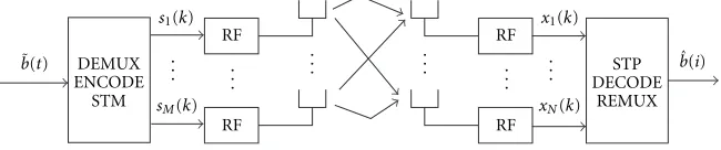
Figure1: A generic (M, N) multiple antenna system.
ber of recently developed STC techniques for multiple-input single-output (MISO) channels, and show what are their attainable capacities. In Section 5, we present similar results for MIMO systems. In Section 6, we show some numerical results for outage capacities of MIMO Rayleigh-faded chan-nels in a number of cases of interest. Finally, in Section 7 we present our conclusions, as well as some directions for future work.
2. BACKGROUND AND ASSUMPTIONS
Figure 1 shows a generic architecture of a wireless system withMtransmitter andNreceiver antennas. Such a system will be denoted in the remainder of the paper as (M, N). The continuous-time input stream ˜b(t) is assumed to be carrying the original primitive data stream{b˜(i)}that is to be com-municated to the receiver. The input stream is then processed by the shown DEMUX/ENCODE/STM unit, whose output is an ensemble ofMparallel data streams, each one of which is separately upconverted and transmitted over the MIMO channel.
The DEMUX/ENCODE/STM unit includes the follow-ing operations:
(1) demultiplexing; (2) encoding;
(3) spatial multiplexing.
These operations may be ordered differently and can be done in a more or less joint fashion. For example, the original bit stream may be encoded first as a whole, and then de-multiplexed onto theMantennas. Alternatively,{˜b(i)}may be first demultiplexed onto a number of sub-streams, each one of which is afterwards separately encoded independently. Either way, the encoded/demultiplexed sub-streams are then mapped through the so-called spatial multiplexer onto the
M antennas for transmission. This mapping may be a sim-ple 1-1 streaming of each encoded sub-stream on each an-tenna (such as in the original so-called V-BLAST transmis-sion mentioned in [8]), or a more complex spatial map-ping. At the receiver, after the signals are received with an antenna array, they are first converted to baseband. Then, they are processed in space and time (STP), decoded, and re-multiplexed in the STP/DECODE/REMUX unit (again the order of these operations may be arbitrary). These opera-tions attempt to recover as reliably as possible a replica of the original primitive bit stream{b˜(i)}. For the purposes of this paper, temporal interleaving is not explicitly accounted for, but it can be easily accomodated.
The way in which we will view MIMO systems through-out the paper is the following. The specific way in which the operations at the transmitter and the receiver mentioned above take place, imposes a number of constraints to the problem of achieving the MIMO capacity. We refer to the system that results after the imposition of these constraints as an architectural “STC structure.” Each STC super-structure then admits a whole class of specific STCs, by ap-plying different types of temporal error-correction codes. Our goal will be to identify what are the capacity penalties inherent to these STC super-structures, due to the imposi-tion of constraints on both the transmitter and the receiver. Said differently, we will attempt to quantify the Shannon ca-pacities that are attainable in each case.
Now we define the notation and assumptions that will be used throughout the rest of the paper. After error correc-tion coding, interleaving, and demultiplexing (irrespective of the order into which these operations occur), the original bit stream {˜b(i)}is converted to a number, say Q, of encoded sub-streams, denoted as{b1(k)}, . . . ,{bQ(k)}. Note that the number of encoded sub-streamsQwill most often equal the number of transmitter antennas M, however this may not always be the case. Finally, the Q sub-streams are mapped through a spatial multiplexing operation, as shown in Figure 1, to theMsub-streams that are transmitted from the
Mantennas. We denote the sub-stream transmitted from the
mth antenna by{sm(k)}. We assume that the physical chan-nel between themth transmitter and thenth receiver antenna is flat-faded in frequency, it can be hence represented, at baseband, through the complex scalarhnm. The baseband re-ceived signal at the receiver antenna array is then represented by the following familiar (narrow-band) mixing model:
x(k)=Hs(k) +n(k), (1) where the involved quantities are defined as follows:
• s(k):=[s1(k) · · · sM(k)]Tis theM×1 vector snapshot of transmitted sub-streams, each assumed of equal varianceσ2
s;
• His theN×Mchannel matrix;
• x(k) is theN×1 vector of received signal snapshots; • n(k) is theN×1 vector of additive noise samples,
as-sumed i.i.d. and mutually independent, each of vari-anceσ2
n.
(M, N) flat-faded channel is given (see [1]) by the now fa-miliar (so-called “log-det”) formula:
C=log2
det
IN + ρ
MHH
† [bps/Hz], (2)
where ρ = Mσ2
s/σn2. This formula assumes the transmitter is constrained to communicate using i.i.d. random processes of equal power from each of theM antennas. Later we will refine the context to fully accommodate an open loop chan-nel outage mode. As mentioned above, the capacity in (2) can be only achieved with the use of strong encoding (STC) techniques. In the remainder of the paper, we will attempt to quantify how much of this capacity is allowed to be attained within certain STC super-structures.
3. FEATURES OF STC ARCHITECTURAL SUPER-STRUCTURES
When viewing (1), the only visible imposed constraints are the equality between the powers of each sub-stream, the in-dependent equal-power noise, and the flat channel charac-teristic. The absence of additional constraints would allow, in theory, the attainable capacity of the (M, N) system to be given by (2). The imposition of further constraints though, reflecting operations at both the transmitter and the receiver, may reduce the capacity in (2). We call this (potentially) re-duced capacity theconstrained capacityof a given architec-tural super-structure.
At the receiver, the received encoded vector signalx(k) is processed in order to produce attempted replicas of the Q encoded sub-streams. These replicas, denoted as
{d1(k)}, . . . ,{dQ(k)}, are then driven to the (joint or
dis-joint) decoder/de-interleaver, which will attempt to recover the original uncoded sub-streams, and eventually, the origi-nal primitive bit stream. Leaving out the encoding/decoding stages, we can take an end-to-end view that relates the en-coded sub-streams at the transmitter {b1(k)}, . . . ,{bQ(k)} to their processed attempted (soft) replicas at the receiver
{d1(k)}, . . . ,{dQ(k)}. Quite often, these relate in a linear
fashion, that is, according to the following model:
d(k)=Fb(k) +v(k), (3) whereFis a square (Q×Q) matrix and all vectors in (3) are of dimension Q×1. We will refer to STC super-structures that admit the end-to-end representation in (3) as end-to-end linear. Further, depend-to-ending on the specific structure and attributes of the mixing matrixFand the noise impairment
v(k), we can define some extra attributes. Before describ-ing these attributes, we define, for convenience, a noise-pre-whitened version of model (3). Denoting byRv the covari-ance matrix ofv(k) (i.e.,Rv = E(v(k)v†(k))), assumed full rank, an equivalent representation of (3) is
d(k)=Fb(k) +v(k), (4) whered(k)=Φ−1
v d(k),F=Φ−v1F,v(k)=Φ−v1v(k), andRv=
E(v(k)v†(k))=ΦvΦ†v. Note that the new noise impairment
v(k) is “spatially” white, that is,E(v(k)v†(k)) =I. We are now ready to define a number of useful properties of end-to-end linear STC super-structures.
Decomposability
We call an end-to-end linear STC super-structure fully de-composable, when the matrixF in (4) is diagonal (possibly after a rearrangement of its entries). In this case, the orig-inal M ×N problem has reduced into Q spatially single-dimensional problems.
Partial decomposability
We call, similarly, an end-to-end linear STC super-structure partially decomposable, when the matrix F in (4) is block-diagonal (again after a possible rearrangement of entries). In other words, instead of a coupledQ×Qproblem, we are faced with a number of decoupled lower-dimension problems.
Balance
We call an end-to-end linear STC super-structurefully bal-anced, when each of the Qsub-streams in (4) experiences the same amount of interference from the otherQ−1 sub-streams as any other sub-stream.
Partial balance
We call an end-to-end linear STC super-structurepartially balanced, when, theQsub-streams can be arranged in groups of sub-streams of dimension lower thanQ, such that each group experiences the same amount of interference from the other groups as any other group of sub-streams.
The features defined above, as well as some other that will be discussed later, will help us classify different STC super-structures, regarding their ability to attain their respective capacities. More precisely, they affect the way in which er-ror correction coding can be embedded in them, so as to approach these capacities. We will now see how some of these properties and features are reflected into some particu-lar STC super-structures.
4. (M,1)SYSTEMS
In this section, we consider some representative STC super-structures that were developed for cases of multiple-input single-output (M,1) systems. Due to the fact that MISO antenna systems provide diversity-type gains, which are, at most, logarithmic inM, (as opposed to the linear capacity in-crease of true MIMO systems), they are usually called “trans-mit diversity systems.” The few techniques that will be shown are examples that fit well within the framework defined in Section 3, and as such, allow for an analytical evaluation of their theoretical constrained capacities. Before proceeding, we mention the open-loop capacity of flat-faded (M,1) sys-tem, which is given by
Cmax
M,1 =log2
1 + ρ
M M
m=1
hm2
which is obtained by substituting, in (2), N = 1 andH =
[h1 · · · hM].
4.1. (2,1)systems: the Alamouti scheme
An ingenious transmit diversity scheme for the (2,1) case was introduced a few years ago by Alamouti [4], and remains to date the most popular scheme for (2,1) systems. We denote bySthe 2×2 matrix whose (i, j) element is the encoded sig-nal going out of the jth antenna at odd (i=1) or even (i=2) time periods (the length of each time period equals the du-ration of one encoded symbol). In other words, one could think of the vertical dimension of Sas representing “time” and of its horizontal dimension as representing “space.” The Alamouti scheme transmits the following signal every two encoded symbol periods: spatial multiplexing is done according to a block scheme, the block length being equal toL =2 time periods. Having as-sumed, as noted earlier, the channel to be flat in frequency, the (2,1) channel is characterized throughH=[h1 h2]. The baseband signal arriving at the single receiver antenna at two consecutive time instants can be expressed as
r(k)=h1 the receiver and complex-conjugating the second output, we obtain match-filtering toH, we obtain
d(k)=H†d(k)
wherev(k) remains spatially white. Comparing to (3), it is clear that this (2,1) system is
1By suitably redefiningc
1andc2, the scheme can be modified for use with direct-sequence CDMA systems, where it is referred to as space-time spreading (STS) [9].
(1) fully decomposable to two (1,1) systems; (2) fully balanced.
The total constrained capacity of the system equals the sum of the capacities of the two SISO systems (recall that each SISO system operates at half the original information rate):
CA2,1=log2
Note that, by contrasting (11) to (5), we see that
C2,1A =C2,1max. (12)
This result is summarized in the following theorem.
Theorem 1. The(2,1)Alamouti transmit diversity scheme has a constrained capacity equal to the(2,1)open-loop channel ca-pacity.2
Moreover, since each component of v(k) is a stationary noise process, the capacity of each (1,1) system is attain-able through conventional (i.e., spatially single-dimensional) state-of-the-art encoding techniques. For example, each of the two sub-streams can be encoded independently with a Turbo code, which is suitable for the classical additive white Gaussian noise channel (with stationary noise).
4.2. A(4,1)scheme
The nice property of the full log-det capacity being attain-able in the (2,1) case does not unfortunately hold in general for (M,1) systems withM >2 (see, e.g., [10, 11]). However, some schemes have been developed recently for special cases. In the following, we describe a scheme that we recently de-rived for the (4,1) case (see [12]) and evaluate its capacity constrained on different receiver processing options.
The original information sequence ˜b(i) is first demul-tiplexed into four sub-streams bm(k) (m = 1, . . . ,4). The 4-dimensional transmitted signal is now organized in blocks ofL=4 (encoded) symbol periods, it is hence represented by a 4×4 matrixS, which is arranged as follows:
where we have dropped the time index k for convenience. The channel matrix is again assumed flat-faded, it can be hence represented byH = h1 h2 h2 h4. The received sig-nal will then be given by
r=S
wherer=[x(1) x(2) x(3) x(4)]Tcontains 4-symbol snap-shots at the received signal. By complex-conjugating the sec-ond and the fourth entry ofrin (14), we obtain
r=
where n is similarly obtained from n by complex-conjugating its second and fourth entry. The received signal is hence written as
r=Hb+n, (16) where nowHis defined as
H=
We now perform matched filtering with respect toH
rmf=H†r=
The parameterαexpresses some residual interference inher-ent in this (4,1) technique, and is in general nonzero. Note both the particular sparse structure of the matrix∆4, as well as the fact thatγis real andαis imaginary. These result in∆4 being in general full rank (det(∆4)=(γ2+α2)2). Comparing (18) to (3), we observe that this (4,1) scheme is:
(1) partially decomposable to two uncoupled (2,2) sys-tems;
(2) fully balanced.
Namely, by grouping the entries ofrmfin two pairs, we obtain
models above share the same 2×2 channel matrix∆2and have identically distributed, but statistically independent, 2×1 ad-ditive noise vectors. In order to facilitate the capacity eval-uation of this scheme, we present at this point the noise-prewhitened version of (20):
independent Gaussian variables of varianceσ2
n each. Again, an identical signal model to (22) holds for the pair{b4, b2}. Similar toγandαin (21),λandκin (23) are real and imagi-nary, respectively. Similarly, the nonzero value ofκrepresents mutual interference between the two sub-streams (ifα =0, thenλ=√γandκ=0).
Maximum allowable Shannon capacity
We first compute the Shannon capacity constrained only upon transmitter processing. By considering the two 2×2 models that describe the post-matched-filtering signals ac-cording to (22), we deduce that the maximum achievable capacity of a (4,1) system within the space-time spreading scheme (13) is given by
C4,1constr,max= 1
wherePT =4σb2is the total average transmitted power from the antenna array (σ2
where ρ = PT/σn2 (all bandwidth-related normalizations have been taken into account, so that (25) represents the total capacity of the system). If the interference caused by the quantity α vanished, the expression in (25) would reduce to
C4,1opt=log21 +ργ
4
(26)
which is the open-loop capacity of the (4,1) flat-faded system. However, for α = 0, Cconstr,max4,1 falls short of
Copt4,1.
4.2.1 Linear receiver processing
We observe from (20) that, in order to demodulate the transmitted sub-streams in a joint fashion, 2 input/2 output multiuser detection (MUD) is required. In this section, we present candidate receivers that perform linear MUD on each pair of matched filter outputs.
Zero-forcing processing
A straightforward way of mitigating the interference in the desired signal bdue toα in (18), is to use a decorrelating (zero forcing—ZF) receiver. Mathematically, the ZF receiver operates on the matched-filter outputs as follows:
rZF=∆−41rmf=b+∆−41nmf. (27)
Due to the decoupling expressed in (20), the ZF operation decouples too, as follows
Note that (28) is equivalent to (27). The ZF receiver detects the four sub-streams by further processing the zero-forcing outputs, that is, the entries of the vectorrZF given in (27). Each of the four zero-forcing outputs can be seen as the out-put of the following AWGN channel:
rZF,i=bi+nZF,i, i=1, . . . ,4, (29)
wherenZF,i is an i.i.d. Gaussian noise independent ofbi, of variance that can be found to equal γσ2
n/(γ2+α2). At this point, the system has been reduced to a fully decomposed, fully balanced system. Hence, its capacity is given by
CZF sub-streams have equal capacities, and that the total capacity of the system equals four times that of any given sub-stream.
MMSE processing
A better compromise between signal recovery and noise am-plification (and hence better performance) can be achieved with minimum mean squared error (MMSE) processing. This is achieved by the 4×4 settingWMS,4which minimizes the MMSE criterion:
min WMS,4
W†
MS,4rmf−b2. (31)
The minimization of (31) yields the Wiener solution
WMS,4† =∆†4
Hence, the post-MMSE-processed signal delivered to the detector is given by
rMS=Ơ4
Similar to the ZF case, the MMSE solution in (33) is, similar to (28), decomposable as follows:3
In this case too, an equation similar to (29) can be written, wherein each sub-stream is detected at the output of a (1,1) system and AWGN noise. The additive noise will contain now contributions from one other sub-stream, it has however the same variance for all four sub-streams. So again, the system has been fully decomposed to four (1,1) systems in a fully balanced way. It is then straightforward to compute the ca-pacity of the MMSE receiver, which is given by
CMMSE
4.2.2 Maximum likelihood MUD
We now focus on the prewhitened signal model (22), which we repeat here for convenience:
Gaussian with covariance matrixσ2
nI2, the maximum likeli-hood (ML) multiuser detector for (37) solves the following optimization problem:
3As expected, asρ→ ∞, the solutionW†
MS,2in (34) converges to the ZF solutionWZF,2† =∆−1
min
{b1,b3}∈Ꮽ×Ꮽ
r1
r3
−Λ
b1
b3
2
, (38)
where Ꮽ is the alphabet shared by all the encoded sub-streams.
Equation (38) is a typical maximum likelihood MUD problem (see [13]). Typically, in order to avoid an exhaus-tive multi-dimensional search, the encoding imparts a spe-cial structure (such as with convolutional codes). Then the use of dynamic programming techniques such as the Viterbi Algorithm (VA) provides an important saving in complexity. We are now ready to assess the capacity of the proposed (4,1) super-structure, constrained on ML reception. Con-sider a pair of transmitted sequences {b˜
1},{˜b3}, to be en-coded in a spatially balanced way (either independently or jointly). Then, because of the symmetrical structure of the channel matrixΛin (37), the communication system is per-fectly balanced (it is understood that the encoding of each sequence at the transmitter is done without knowledge of the channel instantiations). A spatially two-dimensional ver-sion of Shannon’s classical random coding procedure then applies. We start with a primitive (maxentropic) indepen-dent bit stream, and demultiplex it into its even and odd sub-streams,b1 andb3, respectively. The encoded sequence is assigned half of its bits (b1) from the first sub-stream (first dimension), and the other half (b3) from the second sub-stream (second dimension). Then, due to the perfect bal-ance between the two dimensions, the system’s capacity is achieved when each of the two sub-streams achieves its own (half of the full) capacity. This requires, however, joint opti-mal (minimum distance) detection of the two sub-streams, as per (38).
In conclusion, the Shannon capacity which is achieved through ML detection (in the limit of infinitely long random codes) is given by (25), which we repeat here for convenience
CML4,1 =
1 2log2det
I2+ρ 4∆2
. (39)
As will be shown later, this capacity is very close to the full (4,1) capacityCmax
4,1 . Notice that in the ML case, even though it is fully balanced, the system has been only partially decom-posed in two 2×2 systems.
4.3. Nonfull rate(4,1)codes
We now describe some easily derived constrained capacities of some other, less optimal, but quite simple, (M,1) schemes. (1) STS(3,1)—3/4 rate: in [9] it was shown that a (3,1) scheme can be designed, which achieves the full (3,1) capac-ity, but at the price of a 25% loss of rate. This scheme uses block multiplexing, in a fashion similar to the above schemes of Section 4. It multiplexesQ=3 sub-streams on 3 antennas, over L = 4 symbol periods. It results, however, in a fully-decomposable, fully-balanced, 3×3 system with stationary noise. Its constrained capacity is given by
C31−3/4= 3
4log2
1 +ρh1 2
+h22+h32
3
. (40)
(2) STS(4,1)—real: it was also mentioned in [9] and elsewhere, that a fully decomposable and fully balanced extension of the Alamouti (2,1) scheme for real inputs can be used for a (4,1) system. In the case of complex inputs, it is possible to use the same scheme if we sacrifice 50% of the rate, that is by signaling half of the time on each complex di-mension. The capacity of this scheme equals half of the (4,1) open-loop capacity:
C41−real=
1 2C
max
4,1 . (41)
4.4. (M,1)hopping
A very simple alternative that can be used for any integer
M is based on the idea of cycling a single encoded stream over the four transmit antennas. In this case, the data stream is first encoded as a single stream {b(k)}. The encoded se-quence{b(k)}is then demultiplexed intoMsub-sequences,
{b1(k)}, . . . ,{bM(k)}. The mth subsequence is transmitted
from themth antenna (m = 1, . . . , M). In other words, the
M antennas take turns in transmitting (at full power) the
M sub-streams of the single encoded data sequence. This scheme is fully balanced and fully decomposable, however its noise impairment is not stationary. Its capacity is easily found to be given by the average capacity of theMfull-power (1,1) sub-channels, that is,
ChopM,1= 1
M M
m=1
log21 +ρhm2
. (42)
It is important to emphasize that a peculiarity of this simple approach is that the encoded sequence is effectively transmitted through a channel whose SNR is periodic. Con-ventional encoding techniques do not perform in general satisfactorily with such periodic channels. Special codes that can cope with such channels are required in order to be able to approach the capacity in (42). These codes are a current research topic [14].
Discussion
Other approaches for the (M,1) case have appeared in the recent literature. An exhaustive listing of all of them would be however beyond the scope of this paper. We should note further that the benefit of open-loop (M,1) systems becomes increasingly limited asMgrows. Keeping the total transmit power from all the antennas constant, assuming thatE|hm|2= 1 and letting M to grow towards infinity, the (M,1) open-loop capacity in (5) tends to the following asymptote:
C∞,1=log2(1 +ρ). (43)
5. (M, N)SYSTEMS
In this section, we analyze some STC architectural super-structures for the case ofN >1 receiver antennas.
5.1. Combined transmit/receive diversity systems
Given a certain (M,1) system, one straightforward way to de-sign an (M, N) system is to simply:
• transmit as in the (M,1) system,
• receive on each antenna as in the (M,1) system,
• combine optimally theNreceiver antenna outputs.
The capacity quantification of these transmit/receive di-versity systems is straightforward. The M ×N (assumed flat) channel is represented through the N × M channel matrix
We first compute an upper bound for the capacity of such an (M, N) transmit/receive diversity system. With optimal ra-tio combining, and assuming that each (M,1) system takes no interference hit, the input/output relationship takes the form
corresponding to the capacity
Ctrd,maxM,N =log2
It is clear that, when the attainable capacity of the corre-sponding (M,1) schemes is away from the (M,1) log-det ca-pacity, the upper bound in (46) will not be attained either. Notice further that, the expression in (46) is strictly smaller than the (M, N) log-det capacity in (2) forN >1.
Examples
To give some examples, the capacity of a (2, N) system that uses the Alamouti (2,1) super-structure is
CA2,N=log2
that is, as expected, the upper bound in (46) is attained by the Alamouti scheme in the (2, N) case.
It is also straightforward to compute the maximum at-tainable capacity of a (4, N) system that uses the (4,1) scheme of Section 4.2, which is given by
CML4,N=
andΛnis defined, similar to (23) for thenth receiver antenna.
5.2. V-BLAST
A quite simple, from the transmitter’s point of view, STC super-structure was proposed in [8], and is widely referred-to as “V-BLAST.” In this architecture, {(bi)}is first demul-tiplexed intoMsub-streams, which are then encoded inde-pendently and mapped each on a different antenna:
sm(k)=bm(k). (50)
In other words, the original bit stream is converted into a vertical vector of encoded sub-streams (whence the term “vertical” BLAST) which are then streamed to the antennas through a 1-1 mapping. In [8], it was proposed to process the received signal with the use of a successive interference canceller. After determining the order into which theM sub-streams will be detected, the V-BLAST receiver operates ac-cording to the following generic 3-stage scheme, which is fol-lowed in a successive fashion for each sub-stream:
(1) project away from the remaining interfering sub-streams;
(2) detect (after de-coding, de-interleaving, and slicing) the sub-stream;
(3) cancel the effect of the detected stream from sub-sequent sub-streams.
Mathematically, these operations can be described as follows for thekmth sub-stream:
zkm(k)=W
streams will be detected, dec(·) represents the decoding plus detection operation, and enc(·) represents the encoding operation. Finally,Wkmrepresents theN×1 vector that
op-erates on xm(k) in order to project away from sub-streams
{km+1, . . . , kM}. The operations in (51) are performed
suc-cessively for m = 1, . . . , M, after the ordering {k1, . . . , kM} has been determined.
We now discern between the following two cases for this linear operation, since they affect significantly the con-strained capacity of the system.
Zero-forcing projection
are the sub-streams with indices{km+1, . . . , kM}. This nulling is represented mathematically as
WZF,k† mH= 0 · · · 0 1 0 · · · 0=δkm, (52)
where the unique nonzero element of the 1×Mvectorδkmis
in itskmth position. As a result, the end-to-end model for the kmth output is
dkm(k)=bkm(k) +W
†
ZF,kmn(k), m=1, . . . , M, (53)
wheren(k)= n1(k) · · · nN(k)Tis the receiver noise. Defin-ing
d(k)= dk1(k) · · · dkM(k)
T ,
b(k)= bk1(k) · · · bkM(k)
T ,
(54)
equation (53) can be written in matrix form as
d(k)=b(k) +W†ZFn(k), (55) whereWZF= WZF,k1 · · · WZF,kM
. From (55), it is obvious that the ZF version of the V-BLAST super-structure is a fully decomposable, howevernot fully balancedsystem, due to the generally different square norms of the different columns of
WZF.
Regarding the capacity of the end-to-end system, it is im-portant to emphasize that we have assumed that each sub-stream is independently encoded, and that the transmitter has no way of knowing which is the highest rate for each an-tenna. As a result, it can only transmit from all antennas the same rate. Hence, the capacity will equalMtimes the small-est of theMdecomposed channel capacities:
CMNVB-ZF=M×m∈{min1,...,M}
log21 +ρZF,km
, (56)
whereρkmis the output SNR of thekmth sub-stream:
ρZF,km=
ρ
MWZF,kM
2. (57)
It should finally be noted that the capacity in (56) can be optimized by choosing an optimal ordering for the set
{k1, . . . , kM}(see [8]).
MMSE projection
In this case, at themth stage, an optimal compromise be-tween linear interference mitigation of the undetected sub-streams and noise amplification is sought. This is achieved through the following MMSE criterion:
min Wkm
Edkm−W
† kmHkm
2
, (58)
whereHkm is derived fromHby deleting its columns
corre-sponding to indices{k1, . . . , km−1}. This gives forWkm:
WMMSE,k† m=
HkmH † km+
M
ρIN
−1
hkm, (59)
wherehkmis thekmth column ofH. This end-to-end system has now been fully decomposed intoM(1,1) systems, how-ever, it is not generally balanced. Its capacity is hence com-puted again through the minimum of theM1×1 capacities (assuming Gaussian signaling for each sub-stream), and is given by a formula similar to (56):
CVB-MMSE
MN =M×m∈{min1,...,M}
log21 +ρMMSE,km
, (60)
where now
ρMMSE,km =
W†
MMSE,kmHkm
2 MWMMSE,km
2
/ρ+l=k
mWMMSE,l 2. (61)
Again, the capacity in (60) can be maximized through opti-mal ordering.
5.3. Other(M, N)schemes
Similar to the (M,1) case, several other schemes have been proposed in the literature for the general (M, N) case. For example, it was suggested in [15] to use a block space-time multiplexing whose mixing coefficients are derived numer-ically according to a maximum average capacity criterion. Another approach in [16] uses Turbo codes in the follow-ing way: the original sub-stream is first demultiplexed into
M sub-streams, which are separately encoded each with a block code. Then, theMencoded outputs are space-time in-terleaved in a random fashion, mapped onto constellation symbols, and sent out of theMantennas. At the receiver, the
M sub-streams are separated through an iterative interfer-ence canceller, which uses MMSE for the linear (soft) part, and subtracts decisions made after (joint) de-interleaving and (separate) decoding of each interfering sub-stream in the cancellation part.
These approaches have demonstrated encouraging per-formance in terms of bit/frame error rate at the receiver. However, their inherent capacity penalties are still unknown, due mainly to their apparent luck of structure and other properties such as the ones discussed above. The quantifi-cation of the capacity penalties of these and other emerging STC super-structures remains an interesting open question.
6. NUMERICAL RESULTS
0 2 4 6 8 10 12 14 16 18 20 0
1 2 3 4 5 6 7 8 9
2×2 open-loop 2×2 Alamouti
∞ ×1 TD 8×1 TD 4×1 TD 2×1 Alamouti 1×1
Capacit
y
[bps/Hz]
10% outage capacities
SNR [dB]
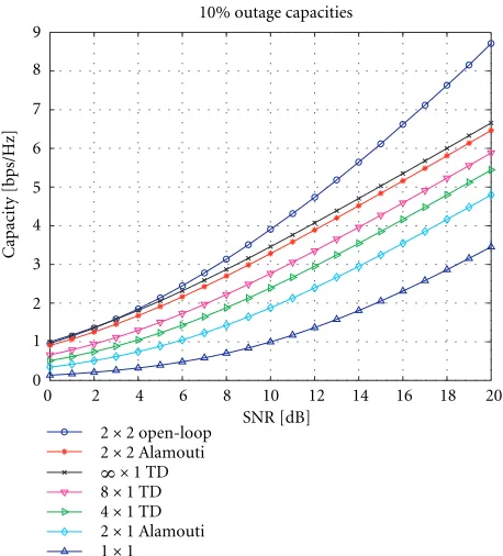
Figure 2: Outage capacities and bounds of (M,1) and (M,2) schemes.
In Figure 2, we show the 10% outage capacities for sev-eral (M,1) cases, as well as for the (2,2) case. In the (2,1) case, the plotted capacity corresponds to both the Alamouti scheme and to the maximum open-loop capacity, as indi-cated by (12). For the other (M,1) cases, we plot the capac-ity upper bounds corresponding to (5), and we use (43) for the asymptotic (∞,1) case. We also use (46) withN =2 for the capacity of a (2,2) combined Alamouti/receive diversity scheme, and the log-det expression (2) for the (2,2) maxi-mum open-loop capacity. We observe that, atρ=10 dB, the (2,1) system almost doubles the capacity of the (1,1) system! However, as noted earlier, increasing the number of transmit antennas in the (M,1) case offers diminishing returns. It is
also worth noting that the (2,2) combined transmit/receiver diversity scheme is capable of attaining a quite significant fraction (particularly at low SNR’s) of the maximum (2,2) open-loop capacity. Finally, it is also interesting to note that a (2,2) system achieves about the same capacity as a (∞,1) system, which conveys again the message of the high value of adding extra antennas at the receiver.
In Figure 3, we show the capacities of the (4,1) scheme of Section 4.2 when used in conjunction with the different pro-posed receiver architectures (ZF, MMSE, and ML). It is no-ticeable that the ML structure approaches closely the chan-nel’s (4,1) open-loop capacity. Moreover, we observe that at low SNR’s, the linear MMSE solution is also very close to the open-loop capacity. Table 1 shows some of these results at chosen SNR points.
Figure 4 shows a comparison of some of the (M,1) sys-tems mentioned in Section 4, including non-full rate variants of the Alamouti (STS) scheme. We observe that the non-full rate schemes fall well behind the (2,1) scheme in terms of
−10 −5 0 5 10 15 20
0 1 2 3 4 5 6
4×1 open-loop capacity 4×1 proposed ML 4×1 proposed MMSE 4×1 proposed ZF
bps/Hz
10% outage capacities
ρ[dB]
Figure3: Outage capacities of the (4,1) scheme of Section 4.2 com-pared to the (4,1) open-loop capacity.
Table1: Indicative outage capacities of the proposed (4,1) scheme versus the (4,1) open-loop capacity.
ρ[dB] ZF MMSE ML OPT
−10 0.038 0.056 0.057 0.057
0 0.344 0.469 0.480 0.491
10 1.886 1.990 2.212 2.339
20 4.805 4.825 5.155 5.379
outage capacity. Moreover, the (2,1) scheme is increasingly close to the (4,1) open-loop capacity at low SNR’s. Similarly, in Figure 5, we show comparative plots of the capacity of the (4,1) hopping scheme mentiond in Section 4.2, (see (42)).
In Figure 6, we show the capacities of some combined transmit/receive diversity schemes for different (4, N) cases. The circles represent the combined (4, N) systems corre-sponding to the (4,1) scheme of Section 4.2, in conjunction with optimal receiver diversity. When read from the bot-tom up, these four curves correspond toN = 1,2,3,4, re-spectively. Similarly, the crosses represent the corresponding open loop (4, N) capacities. Notice that the proposed (4,1) scheme is very close to the open-loop capacity, however the gap gets increasingly larger asN grows from 1 to 4. In the (4,2) case however, the scheme still performs very well at low SNR’s.
−10 −5 0 5 10 15 20 0
1 2 3 4 5 6
4×1 open-loop capacity 4×1 proposed ML 4×1 proposed MMSE 2×1 STS
3×1 STS 3/4 4×1 STS real
10% outage capacities
bps/Hz
ρ[dB]
Figure4: 10% outage capacities compared to other open-loop al-ternatives.
−10 −5 0 5 10 15 20
0 1 2 3 4 5 6
4×1 open-loop capacity 4×1 proposed ML 4×1 hopping
bps/Hz
10% outage capacities
ρ[dB]
Figure5: Outage capacity of a hopping scheme.
architecture attains only about 50% of the (4,4) open-loop capacity, whereas the ZF architecture is outperformed by the (1,4) system across the board.
7. CONCLUSIONS
We have presented a framework for analyzing space-time coding architectures in terms of Shannon capacity. We de-fined a number of attributes of such schemes that allow
−10 −5 0 5 10 15 20
0 2 4 6 8 10 12 14 16 18 20
4×1 open-loop 4×1 proposed max 4×2 open-loop 4×2 proposed max 4×3 open-loop 4×3 proposed max 4×4 open-loop 4×4 proposed max
bps/Hz
10% outage capacities
ρ[dB]
Figure 6: Outage capacities of the (4,1) scheme described in Section 4.2, when used with up to four receiver antennas.
0 2 4 6 8 10 12 14 16
0 0.1 0.2 0.3 0.4 0.5 0.6 0.7 0.8 0.9 1
(1,4) open-loop (4,4) V-BLAST-ZF (4,4) V-BLAST-MMSE (4,4) open-loop
Pr
(c
ap
ac
it
y
>
abcissa)
M=4,N=4,ρ=10 dB
Capacity [bps/Hz]
Figure7: Outage capacity distribution of a V-BLAST MMSE archi-tecture at 10 dB SNR.
0 1 2 3 4 5 6 0
0.1 0.2 0.3 0.4 0.5 0.6 0.7 0.8 0.9 1
(1,4) open-loop (4,4) V-BLAST-ZF (4,4) V-BLAST-MMSE (4,4) open-loop
Pr
(c
ap
ac
it
y
>
abcissa)
M=4,N=4,ρ=0 dB
Capacity [bps/Hz]
Figure8: Outage capacity distribution of a V-BLAST MMSE archi-tecture at 0 dB SNR.
capacity. We believe that these results provide some useful intuition regarding the performance trade-offs of different techniques. Future work will be targeted in analyzing other promising STC schemes, as well as in determining new ar-chitectures of higher capacity potential.
REFERENCES
[1] G. J. Foschini, “Layered space-time architecture for wireless communication in a fading environment when using multi-element antennas,” Bell Labs Technical Journal, vol. 1, no. 2, pp. 41–59, 1996.
[2] C. Berrou, A. Glavieux, and P. Thitimajshima, “Near Shannon-limit error correction coding and decoding: Turbo codes,” inProc. 1993 International Conference on Communi-cations, pp. 1064–1070, Geneva, Switzerland, May 1993. [3] C. Shannon, “A mathematical theory of communication,”Bell
System Technical Journal, vol. 27, pp. 379–423, 623–656, 1948. [4] S. Alamouti, “A simple transmitter diversity scheme for wire-less communications,”IEEE Journal on Selected Areas in Com-munications, vol. 16, no. 8, pp. 1451–1458, 1998.
[5] V. Tarokh, N. Seshadri, and A. R. Calderbank, “Space-time codes for high data rate wireless communication: perfor-mance criterion and code construction,” IEEE Transactions on Information Theory, vol. 44, no. 2, pp. 744–765, 1998. [6] C. Papadias, “On the spectral efficiency of space-time
spread-ing schemes for multiple antenna CDMA systems,” in33rd Asilomar Conference on Signals, Systems, and Computers, pp. 639–643, Pacific Grove, Calif, USA, October 1999.
[7] S. Sandhu and A. Paulraj, “Space-time block codes: a capacity perspective,”IEEE Communications Letters, vol. 4, no. 12, pp. 384–386, 2000.
[8] G. J. Foschini, G. D. Golden, R. A. Valenzuela, and P. W. Wol-niansky, “Simplified processing for wireless communication at high spectral efficiency,” IEEE Journal on Selected Areas in Communications, vol. 17, no. 11, pp. 1841–1852, 1999. [9] B. Hochwald, L. Marzetta, and C. Papadias, “A transmitter
di-versity scheme for wideband CDMA systems based on space-time spreading,”IEEE Journal on Selected Areas in Communi-cations, vol. 19, no. 1, pp. 48–60, 2001.
[10] A. V. Geramita and J. Seberry, Orthogonal Designs: Quadratic Forms and Hadamard Matrices, Marcel Dekker, New York, USA, 1979.
[11] G. Ganesan and P. Stoica, “Space-time diversity using or-thogonal and amicable oror-thogonal designs,” inProc. IEEE Int. Conf. Acoustics, Speech, Signal Processing, Istanbul, Turkey, June 2000.
[12] C. Papadias and G. J. Foschini, “A space-time coding approach for systems employing four transmit antennas,” in Interna-tional Conference on Acoustics, Speech, and Signal Processing, Salt Lake City, Utah, USA, May 2001.
[13] S. Verd ´u, Multi-User Detection, Cambridge University Press, Cambridge, UK, 1999.
[14] R. D. Wesel, X. Liu, and W. Shi, “Trellis codes for periodic era-sures,” IEEE Trans. Communications, vol. 48, no. 6, pp. 938– 974, 2000.
[15] B. Hassibi and B. Hochwald, “High-rate linear space-time codes,” inProc. IEEE Int. Conf. Acoustics, Speech, Signal Pro-cessing, Salt Lake City, Utah, USA, May 2001.
[16] M. Sellathurai and S. Haykin, “Joint beamformer estimation and co-antenna interference cancelation for turbo-BLAST,” in
Proc. IEEE Int. Conf. Acoustics, Speech, Signal Processing, Salt Lake City, Utah, USA, May 2001.
Constantinos B. Papadias was born in Athens, Greece, in 1969. He received the diploma of electrical engineering from the National Technical University of Athens (NTUA) in 1991 and the Ph.D. degree in signal processing (highest honors) from the Ecole Nationale Sup´erieure des T´el´e-communications (ENST), Paris, France, in 1995. From 1992 to 1995, he was a Teaching and Research Assistant at the Mobile
Com-munications Department, Eur´ecom, France. In 1995, he joined the Information Systems Laboratory, Stanford University, Stanford, Calif, USA, as a PostDoctoral Researcher, working in the Smart An-tennas Research Group. In November 1997, he joined the Wireless Research Laboratory of Bell Labs, Lucent Technologies, Holmdel, NJ, USA, as a Member of Technical Staff. He now heads the Global Wireless Strategy Research group in the same lab. His current re-search interests lie in the areas of multiple antenna systems (e.g., MIMO transceiver design, and space-time coding), interference mitigation techniques, reconfigurable wireless networks, as well as financial evaluation of wireless technologies. He has authored sev-eral papers and patents on these topics. Dr. Papadias is a member of the Technical Chamber of Greece.
Gerard J. FoschiniBSEE-NJIT, MEE-NYU, Ph.D. Mathematics-Stevens. Mr. Gerard J. Foschini has been at Bell Laboratories for nearly 40 years. He holds the position of Distinguished Member of Staff. He has con-ducted data communications research on many kinds of systems, most recently wire-less communications and optical communi-cations systems. Gerard has done extensive research on point to point systems as well as