Effect of SC on frequency content of geomagnetic data using DWT application:
SC automatic detection
Essam Ghamry1,2, Ali G. Hafez1,3, Kiyohumi Yumoto4, and Hideki Yayama3,5
1National Research Institute of Astronomy and Geophysics, (NRIAG), Helwan, 11722, Egypt 2Space Weather Monitoring Center (SWMC), Helwan University, Ain Helwan 11795, Egypt
3LTLab Inc., Kyushu University, Hakozaki 6-10-1, Japan
4Space Environment Research Center, Kyushu University, Hakozaki 6-10-1, Japan 5Department of Physics, Faculty of Sciences, Kyushu University, Hakozaki 6-10-1, Japan
(Received July 14, 2011; Revised April 26, 2013; Accepted April 30, 2013; Online published October 9, 2013)
In this paper, a study is made to determine the effect of sudden commencement (SC) on the power spectrum of geomagnetic data using multiresolution analysis (MRA) of the discrete wavelet transform (DWT). The results of this study provides a guide to develop a new technique to automatically detect the SC because it could be an indicator of the onset of a geomagnetic storm. This new technique divides the original time series into different frequency sub-bands using the MRA of the DWT. Then it detects the change in a certain sub-band which shows a large change due to the SC. The geomagnetic records used in this study were 3-s resolution data collected from the Circum-Pan Pacific Magnetometer Network (CPMN). Using such high-resolution data enables us to minimize the detection error and the processing time to make a decision. The proposed algorithm is tested on one sample every three seconds of data sets collected from the CPMN. The maximum standard deviation of the algorithm detection times is observed to be fifty four seconds of the corresponding arrival times as determined by the National Geophysical Data Center (NGDC).
Key words:Automatic detection, geomagnetic storms, DWT, sudden commencement, CPMN.
1.
Introduction
It is known that a geomagnetic storm is one of the most prominent phenomena in the geospace environment. Moos (1910) identified a well-defined pattern in the so called “X disturbance” in the horizontal component (H-component) at Colaba, India. He found an occasional sudden rise of the horizontal component followed by a rapid decrease lasting a few hours and a slow recovery lasting 2–3 days. These disturbances are defined as “magnetic storms” and the var-ious phases of the storm have been named by Chapman (1918) and Araki (1994) as: (i) sudden storm commence-ment (SC); (ii) initial phase; (iii) main phase; and (iv) the recovery phase.
The Dst index is commonly used in studies of magnetic storms as an indicator of the intensity of the ring current or magnetic storms. It is known that the SC is not a necessary condition for a storm to occur, and hence the initial phase is not an essential feature. But the essential feature of a storm is the significant development of a ring current.
The term Sudden Impulse (SI) is used for a sudden in-crease in the H-component without an ensuing magnetic storm. SIs were first regarded as magnetic disturbances with a different nature from SCs. However, SIs have been proved to be caused by the same physical mechanisms as SCs and should be classified as being complementary to SCs
accord-Copyright cThe Society of Geomagnetism and Earth, Planetary and Space Sci-ences (SGEPSS); The Seismological Society of Japan; The Volcanological Society of Japan; The Geodetic Society of Japan; The Japanese Society for Planetary Sci-ences; TERRAPUB.
doi:10.5047/eps.2013.04.006
ing to Curtoet al.(2007).
The automatic detection of sudden commencements which are followed by magnetic storms is of great impor-tance, as these events often affect radio and television inter-ference and blackouts, which are hazards to orbiting astro-nauts and spacecrafts and power grids.
Joselyn (1985) has pointed out the need for an automatic detection of SC in real time to alert forecasters of poten-tial geomagnetic storm conditions. Mendeset al. (2005) detected variations of the H-component of the geomagnetic field related to geomagnetic storms by means of wavelets. Shinoharaet al. (2005) developed an automatic real-time detection and warning system of geomagnetic sudden com-mencements using real-time data from ground-based geo-magnetic observations.
They developed a method based on statistical analysis to detect the SCs using the amplitude and increasing rate of the geomagnetic field. The forecasting of magnetic storms by using a moving gradient of the SYM-H index (the sym-metric portion of the horizontal component of the mag-netic field) as a detecting algorithm has been pointed out by Khabarovaet al.(2006).
The automatic detection of the onset time of natural events is common in the literature. Hafez et al. (2009, 2010) used a spectrogram and a DWT, respectively, to de-tect earthquake onset arrival times. Takanoet al. (1999) used lifting wavelet filters to build an SC detection algo-rithm for one-minute data resolution recorded at the KAG station. Hafez and Ghamry (2011) used time-frequency clusters to automatically detect SC times applied on
1008 E. GHAMRYet al.: EFFECT OF SC ON FREQUENCY CONTENT OF GEOMAGNETIC DATA USING DWT
Table 1. List of magnetic observatories used in our study.
Station Name Code Geographic Geomagnetic
Lat. N Long. E Lat. N Long. E
Onagawa ONW 38.43 141.47 31.15 212.63
Kuju KUJ 33.10 131.20 26.03 202.90
Kagoshima KAG 31.48 130.72 24.37 202.36
minute data resolution and compared their algorithm with that of Takanoet al.(1999). In this paper, we introduce a new algorithm to automatically detect SC times for three-second resolution data. The algorithm proposed by Hafez and Ghamry (2011) cannot be used for the three-second resolution data as the frequency content is totally different from the frequency content of the one-minute data.
Motivated by these facts, an algorithm for the automatic detection of geomagnetic sudden commencements is intro-duced using the details of multiresolution analysis (MRA) of a discrete wavelet transform (DWT). In the proposed algorithm, discrete wavelet coefficients of segments con-taining SCs are calculated at different scales. Using these coefficients, detailed features at each scale are determined. Among these details, we choose the second-stage detail in detecting SC because in this detail the arrival is very clear which enables us to detect the SC time correctly.
2.
Multiresolution Analysis (MRA)
One of the important features extracted from DWT is the multiresolution analysis (MRA). MRA charac-terizes the spectrum of the signal at each DWT scale into low-frequency features, approximations (A), and high-frequency contents which are the details (D). Many algo-rithms are dedicated to determine approximations, Aj, and
details, Dj, of the MRA of DWT. A pyramid algorithm is
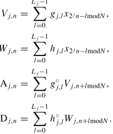
one of these algorithms described by Percival and Walden (2000). In this algorithm scaling,Vj,n, and wavelet,Wj,n,
coefficients at each stage (j) of DWT stages are calculated using the following equations:
are scaling and wavelet filters respectively, where j is the stage number andLis the filter width. The scaling filtergl
is a quadrature mirror filter that corresponds to the wavelet filterhl by the equation gl = (−1)l+1hL−1−l; the inverse
relationship ishl =(−1)lgL−1−l.{gl◦}is{gl}periodized to
lengthN,{hl◦}is{hl}periodized to lengthNand ‘amodb’
stands for ‘amodulob’.
x(n)is the input time series,n=0,1, ...,N2 −1.
Fig. 1. Map of the sites used to collect data to test the proposed algorithm.
The original time series can be reconstructed using the following equation:
xn=D1,n+D2,n+...+Dj,n+Aj,n
3.
Data Set
In this study, 93 sudden commencements followed by ge-omagnetic storms are checked. These events occurred be-tween May 1992 and September 2005 based on the National Geophysical Data Center (NGDC) of the National Oceanic and Atmospheric Administration (NOAA). Checked events are 3-second resolution of H-component (northward com-ponent) data at a low latitude from the Circum-pan Pacific Magnetometer Network (CPMN). The CPMN was con-structed by Kyushu University in collaboration with about 30 international organizations along the 210◦ magnetic meridian and magnetic equator during the international So-lar Terrestrial Energy Program (STEP) period (1990–1997). The principle investigator (PI) of the CPMN project is Pro-fessor K. Yumoto. Figure 1 and Table 1 show the location of the stations used for this paper.
4.
Effect of SC on Geomagnetic Data Spectrum
SC, as a change in the geomagnetic record, results in an increase in the power of all spectrum bands at the time of its occurrence. The amount of the power increase in each fre-quency sub-band depends on the rate of variation of the SC. The traditional parameter which describes the sharpness of an SC is the maximum time variation of the SC (Shinohara
high-Fig. 2. Maximum time variation is calculated over the total period of the SC increase.
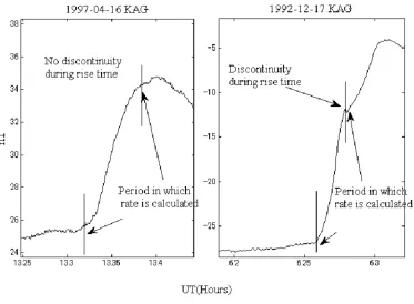
Fig. 3. Enlarged window of the H-component around the SC and the period in which the rate of variation is calculated. In the left subfigure, we can notice that there is no discontinuity in the trace. In the right subfigure, a discontinuity in the trace can be recognized. The rate is calculated in the period between the vertical lines drawn in each subfigure.
and low-frequency regions the consequence of which is that the calculation of this parameter over the entire period does not precisely represent the rate of SC increase. The high-frequency region is the region where there is a fast rate of change of the geomagnetic field. While the low-frequency range is the region where there is a slow rate. The division of these two regions was accomplished manually, where by
1010 E. GHAMRYet al.: EFFECT OF SC ON FREQUENCY CONTENT OF GEOMAGNETIC DATA USING DWT
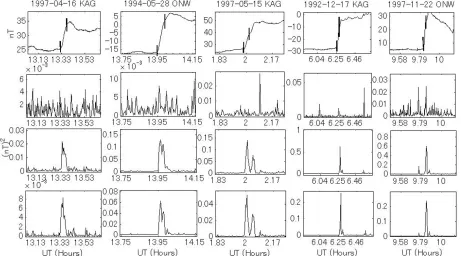
Fig. 4. Five SCs with rather small rates of variation. The first row is the H-component of the five SCs in the time domain. The second to fourth row each contains the corresponding averaged squared first to third detail of each SC, respectively.
is a change from the high-frequency, to the low-frequency, region. This high-frequency region occurs within two min-utes of the SC arrival. This way of calculating the SC rate of variation defines the sharpness of the SC precisely.
In Fig. 3, there are two SCs recorded at the KAG station: the first one was recorded on April 16, 1997, while the second SC was on December 17, 1992. In the first SC we can recognize that the trace has no discontinuity starting from the arrival time of this SC to the end of its rise time. The rate of variation of this SC can be calculated using the period between the two vertical lines which are drawn in the first SC. For the second SC, a discontinuity can be recognized in the trace during the rise time. Therefore, the rate of variation for the second SC is calculated over the trace between the two vertical lines which are drawn on the second SC. The rates of variation for the first and second SCs are 0.17 and 0.62 nT/sample, respectively, where the sampling rate is one sample per three seconds.
In order to investigate the effect of the SC on the power increase at different scales (frequencies), MRA details of DWT (first to third) of geomagnetic signals are calculated using the Daubechies wavelet filter of order 4 (abbreviated as db4). Each detail is squared, then the average of each five samples is calculated to reduce ripples in the record. As a result of this averaging process, the length of the aver-aged detail will be equal to the length of the original record divided by five. Figure 4 contains five columns and each column has four windows. The H-components of five dif-ferent SCs in the time domain are located at the top of each column in the first row. The other three windows in each column, second, third and fourth row, are the correspond-ing averaged squared three details of the SC, first to third, respectively. A full explanation for each SC is given in the following.
The first window of the first column is an SC recorded at the KAG station on April 16, 1997. The arrival time of this SC in the time domain is at 13.33 UT. In the second window of the first column, we note no change in the power of the first detail around 13.33 UT. On the other hand, in the third and fourth windows of the first column, the power of the second and third details around 13.33 UT show a clear increase. The rate of variation of this SC is 0.17 nT/sample. The SC at the top of the second column was recorded at the ONW station on May 28, 1994. The arrival timing of this SC is around 13.95 UT. Similarly to the first SC, although there is no change in the power of the first detail around 13.95 UT, a significant increase in power is observed in the second and third details around 13.95 UT. The rate of variation of this SC is 0.4 nT/sample.
In the same fashion, the third SC in the third column, which was recorded at the KAG station on May 15, 1997, the arrival time is around 01.99 UT. Although there is no change in the power of the first detail, around 01.99 UT, there is a clear increase in the power of the second and third details. The rate of variation of this SC is 0.4 nT/sample.
The SC in the fourth column was recorded at the KAG station on December 17, 1992. The arrival time is at 06.25 UT, a slight increase in power of the first detail around 06.25 UT can be recognized where as a large increase in the power of the second and third details around 06.25 UT is detected. The rate of variation of this SC is 0.62 nT/sample.
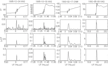
Fig. 5. Four SCs with a rather higher rate of variation values than the SCs of Fig. 4. The first row is the H-component of the geomagnetic field of the four SCs in the time domain. The second to fourth row each contains the corresponding averaged squared first to third detail of each SC, respectively.
can conclude that the SCs with a low rate of variation do not result in a change in the power of the first detail, which is found in the frequency band 41.67–83 mHz. A clear change in the power of the second and third details can be detected due to the same low-rate SCs. The frequency bands of the second and third details are 20.8–41.67 mHz and 10.38– 20.8 mHz, respectively. With the increase of the rate of variation of SCs, a slight increase in power of the first detail can be recognized as shown in the first detail of the fourth and fifth SCs of Fig. 4.
In Fig. 5 SCs with a high rate of variation are shown. The rate of variation values of the SCs in Fig. 5, starting from left to right, are 1, 1.07, 1.32 and 3.85 nT/sample, respectively. We can recognize that the level of increase of the power of the first detail during the SC is in direct proportional to the rate of variation of this SC. So that we can say that, with a higher SC rate of variation, the increase in power of the first detail will be more recognized.
5.
SC Automatic Detector
There are advantages of building an SC automatic detec-tion algorithm using high-resoludetec-tion data instead of the one-minute data adopted by Shinoharaet al.(2005), Hafez and Ghamry (2011) and others. The first advantage is a reduc-tion of the automatic detecreduc-tion error. Assuming that both algorithms made an error of two samples in detection, in the former study, using a one-minute sampling data, this re-sulted in a 120-s error, whereas in the present study, with a 3-s sampling data, it involved a 6-s error. The second advan-tage is a reduction of the automatic detection delay. In the algorithm proposed by Shinoharaet al.(2005) the decision is given based on three parameters, which are the ampli-tude, the time required for the increase and maximum time
variation, which means that the delay is more than the time required for an increase which ranges from 2–10 minutes. Hafez and Ghamry (2011) used a four-samples window to search for an SC, which means a four-minute delay after receiving the data from the stations. In our proposed algo-rithm, the window is five samples which means 15 seconds delay after receiving the data. Therefore, it is favorable to use high-resolution data to perform fast and accurate SC detection.
The rule of MRA of DWT is to create the frequency sub-bands. Where the details represent the high-frequency components, and the approximations are the low-frequency components, of each stage. Therefore, details may be con-sidered as the original signal filtered within a specific band-width, which can be calculated from the equation 2Fj+1 ≤
|F| ≤ 2Fj, where F is 166*10−3 Hz as the sampling rate
1012 E. GHAMRYet al.: EFFECT OF SC ON FREQUENCY CONTENT OF GEOMAGNETIC DATA USING DWT
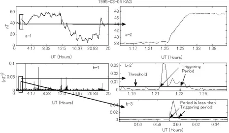
Fig. 6. Methodology of how the algorithm alarms for a trigger. The alarm for one record is set when the amplitudes of the averaged squared second detail exceed the triggering threshold over a period longer than the triggering period. The detailed explanation for each panel is described in the text.
calculated to reduce any ripple which may cause false detec-tions. A trigger is declared when the amplitude of this aver-aged squared detail exceeds a certain threshold over a cer-tain triggering period. The values of the triggering thresh-old and period are chosen after checking many SCs. One of these SCs is shown in Fig. 6.
In Fig. 6, a-1 and a-2 show the H-component of the ge-omagnetic field for an entire day and the enlarged segment of this field around SC, respectively. b-1 is the averaged squared second detail of the entire day. In (b-2), the seg-ment around the SC in the second detail is enlarged. In this subfigure, we can notice that the condition of alarming for a trigger is satisfied when the amplitudes of the second detail exceed the triggering threshold over a period larger than the triggering period.
In (b-3), a spike during which the amplitude exceeds the threshold can be seen. This spike doesn’t alarm for a trig-ger as the duration of such a spike is less than the trigtrig-ger- trigger-ing period. There is a possibility of the occurrence of the alarming condition when there is no SC; in such a situation, this trigger is called a false trigger. This possibility, of false triggers, is low in normal days but it is observed to increase after the occurrence of an SC. In order to confirm that this trigger is an SC and not a false trigger, the other stations are checked if they alarm for a trigger within a certain pe-riod around the time of this alarm. If a trigger is found at these stations, this trigger is declared to be an SC, otherwise this trigger is declared as a false trigger. This certain period is considered as an accepted margin, and can be set by the user. In this paper, we propose three minutes for this spe-cific period. Examples explaining this point in detail will be described in the Section 6, and are shown in Table 2.
6.
Results
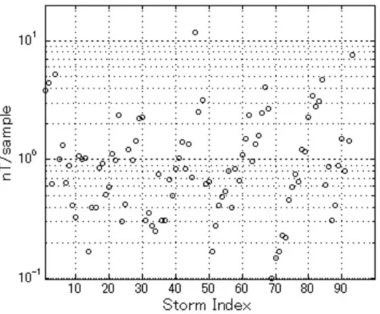
The data set collected from the CPMN is chosen to sat-isfy different values of the SC rate of variation which is explained in Section 4. The smaller this rate of variation is, the harder it is to automatically detect the SC arrival time correctly. Figure 7 shows a plot of the rate of variation val-ues of all SCs which have been used to test the proposed algorithm. In this figure, we can see that the values of the rate of variation range from 0.1 to 11.8 nT/sample.
The proposed SC detection algorithm was tested for 93 magnetic storms, recorded by the stations listed in Table 1. The SC times calculated by the present algorithm are com-pared with the times listed in the web-site of the National Geophysical Data Center (NGDC) of the National Oceanic and Atmospheric Administration (NOAA). It was found that unsuccessful detections were only eight SCs, which is a small number.
Figure 8 illustrates the error probability distribution func-tion when using a db4 wavelet filter, where the error is de-fined as the time difference between the algorithm arrival times and the SC times which are determined by the NGDC. The average and standard deviation of error are found to be 1 and 18 samples, respectively, where the sampling rate is one sample per three seconds.
Fig. 7. The rate of variation values of the 93 SCs which are used in this study.
Fig. 8. The probability distribution function (PDF) of the error in detection times generated by the algorithm compared with NGDC times. Negative values means the detection time made by the algorithm leads the NGDC detection.
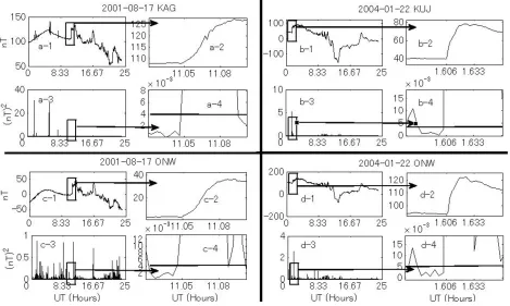
SC, a-2 is an enlarged view of the SC, a-3 is the squared av-eraged second detail of the entire day, and a-4 is an enlarged window around SC of the averaged squared second detail. The other three SCs (b, c and d) are arranged in the same manner. In each of the four subfigures a, b, c and d-4, we can recognize that the amplitudes of the averaged squared second detail exceed the threshold over a period, which is larger than the triggering period which results in triggering for an SC at the arrival time of the SC.
Table 2 contains some examples of the SCs used to test the proposed algorithm. In Table 2, we can find that there are two or three stations which record the same SC. It is clear that the Algorithm Detection Times of the stations
1014 E. GHAMRYet al.: EFFECT OF SC ON FREQUENCY CONTENT OF GEOMAGNETIC DATA USING DWT
Fig. 9. Four examples from the used data set. The subfigures can be explained as follows: a-1 and a-2 are the H-component of the geomagnetic field of the entire day and the enlarged segment of this field around SC, respectively. a-3 and a-4 are the averaged squared second detail of the entire day and the enlarged segment of this detail around SC, respectively. The same sequence is valid for b, c and d.
Table 2. Arbitrarily chosen SCs from the checked data set. These examples show the capability of the algorithm to determine the SC timing correctly and its immunity against alarming false triggers. Times are expressed in UT of the respective days and in units of sample (1 sample=3 s).
Serial Date and station Arrival times of SCs Algorithm detection times Error Rate of variation
by the NGDC (samples) (samples) of SC
1 2001-08-17 KAG 13260 13255, 15930, 19705, 24380, 25025 −5 0.5
2 2001-08-17 ONW 13260 13250, 13335, 13680, 14155, 14390 −10 0.84
3 2004-01-22 KUJ 1928 1925, 2000, 2150, 2525, 2640 −3 4.06
4 2004-01-22 ONW 1929 1925, 2005, 2150, 2390, 2510 −4 2.68
5 2004-08-29 KUJ 12110 12145, 18210 35 0.23
6 2004-08-29 ONW 12110 12145 35 0.22
7 2004-12-05 KAG 9327 1765, 7080, 9325, 9670, 10510 −2 0.65
8 2004-12-05 KUJ 9328 9325, 9395, 9635, 9700, 10300 −3 1.22
9 2004-12-05 ONW 9335 9365, 10585, 10630, 11815, 19155 30 1.16
10 2005-01-21 KAG 20630 4770, 13010, 13725, 20395, 20605 −25 2.29
11 2005-01-21 KUJ 20630 20600, 20715, 20845, 21050, 21340 −30 3.46
12 2005-01-21 ONW 20630 5250, 20610, 20755, 21055, 21290 −20 2.8
7.
Conclusions
The effect of sudden commencement on geomagnetic data spectrum is investigated in this paper using the DWT. This effect provided the guide to build a new algorithm for determining geomagnetic storm sudden commencement onset times. It is proved that the change in the spectrum during the SC is directly proportional to the value of the SC rate of variation. Investigations elaborate that the second detail of the MRA of the DWT is the best detail to be used to monitor the SC timing. Case studies have shown that the algorithm is very sensitive to both low- and high-rate variation SCs. Applying the algorithm on a data set from the Circum-pan Pacific Magnetometer Network (CPMN), it is found that the time of SC arrivals computed by our
proposed algorithm is very close to those observed by the NGDC.
Acknowledgments. The results presented in this paper rely on data collected from the Circum-pan Pacific Magnetometer Net-work (CPMN). The authors would like to thank the staff members of CPMN.
Appendix A.
This appendix contains the pseudo code of the proposed algorithm as follows:
Read the H-component record
Set the detection threshold amplitude Set the triggering period
While the segment number is less than total number of segments
Calculate the DWT squared second detail of the current segment
If the average value of the squared second detail is larger than the detection threshold over a pe-riod greater than the triggering pepe-riod
Calculate the timing of the segment Display that there is an SC in this record else
Display that there is no SC in this record End if
Add one to segment
End while
Read reference value of SC which is published by NGDC
Define the error which is the difference between the cal-culated SC timing and the reference timing published by NGDC
References
Araki, T., A physical model of the geomagnetic sudden commencement,
Geophysical Monograph,81, 183–200, 1994.
Chapman, S., On the times of sudden commencements of magnetic storms,
Proc. Phys. Soc.,30, 205–214, 1918.
Curto, J. J., T. Araki, and L. F. Alberca, Evolution of the concept of Sudden Storm Commencements and their operative identification,Earth Planets Space,59, i–xii, 2007.
Hafez, A. G. and E. Ghamry, Automatic detection of geomagnetic sudden commencements via time frequency clusters,Adv. Space Res.,48, 1537– 1544, 2011.
Hafez, A. G., T. A. Khan, and T. Kohda, Earthquake onset detection using spectro-ratio on multithreshold time-frequency sub-band,Digital Signal Process., 19(1), January 2009, 118–126, 2009.
Hafez, A. G., T. A. Khan, and T. Kohda, Clear P-wave arrival of weak events and automatic onset determination using wavelet filter banks,
Digital Signal Process,20(3), May 2010, 715–723, 2010.
Joselyn, J. A., The automatic detection of geomagnetic-storm sudden com-mencements,Adv. Space Res.,5(4), 193–197, 1985.
Khabarova, O., V. Pilipenko, M. J. Engebretson, and E. Rudenchik, Solar wind and interplanetary magnetic field features before magnetic storm onset,Proc. Of International Conference of Substorms,8, 1–6, 2006. Mendes, O. J., M. O. Domingues, A. M. da Costa, and A. L. Clua de
Gonzalez, Wavelet analysis applied to magnetograms: Singularity de-tections related to geomagnetic storms,J. Atmos. Sol.-Terr. Phys.,67, 1827–1836, 2005.
Moos, N. A. F., Magnetic observations made at the government observa-tory Bombay 1846–1905 and their discussion. Part II,The Phenomenon and Its Description, 1910.
Percival, D. B. and A. T. Walden,Wavelet Methods for Time Series Analy-sis, Cambridge: Cambridge University Press, 2000.
Shinohara, M., T. Kikuchi, and K. Nozaki, Automatic realtime detection of sudden commencement of geomagnetic storms,J. NICT,52(3/4), 197– 205, 2005.
Solar-Geophysical Data, http://sgd.ngdc.noaa.gov/, National Geophysical Data Center (NGDC), NOAA.
Takano, S., T. Minamoto, H. Arimura, K. Niijima, T. Iyemori, and T. Araki, Automatic detection of geomagnetic sudden commencement using lift-ing wavelet filters,Lecture Notes in Computer Science, Springer Berlin / Heidelberg Volume 1721, 1999.