Patrick David Bangert
A lgorith m ic P rob lem s
in th e B raid G roups
Subm itted for th e degree of Ph.D . Supervisor: P ro f M itchell A. Berger
D epartm ent of M athem atics University College London
Gower Street London W C IE 6B T
U nited Kingdom
ProQ uest Number: U6 4 3 8 4 1
All rights reserved
INFORMATION TO ALL U SE R S
The quality of this reproduction is d ep en d en t upon the quality of the copy subm itted.
In the unlikely even t that the author did not sen d a com plete manuscript and there are m issing p a g e s, th e se will be noted. Also, if material had to be rem oved,
a note will indicate the deletion.
uest.
ProQ uest U 6 4 3841
Published by ProQ uest LLC(2016). Copyright of the Dissertation is held by the Author.
All rights reserved.
This work is protected against unauthorized copying under Title 17, United S ta tes C ode. Microform Edition © ProQ uest LLC.
ProQ uest LLC
789 East E isenhow er Parkway P.O. Box 1346
A b stract
This is dedicated to all those who, in the face of adversity, throw themselves headlong into the battlefields and fight until they achieve victory or die trying.
”It is tim e I focused on my problem. W ho does not have a problem ? — Everybody has one, and indeed several. Each problem has its rank; the m ain problem moves to the center of one’s life, displacing the other problems. It incessantly haunts us like a shadow, casting gloom on our minds. It is present even when we awaken a t night; it pounces on us like an animal. ... W hen I stir my m orning coflFee and watch the swirling of th e streaks, I am observing the law th a t moves the universe — in the whirling of the spiral nebulae, in th e eddying of th e galaxies. ... B ut w hat does it m atter? W hether the universe whirls or crumbles — the problem remains behind it. ... The problem is indivisible; m an is alone. Ultimately, one cannot rely on society. A lthough society usually wreaks harm , indeed often havoc, it can also help, although no t more th a n a good physician — up to the inevitable limit where his skill fails. ... My tim e is limited; b u t anyone can spend a m onth retreating into the forest or the desert. There, he can describe — or better: circumscribe his problem; it is th en defined, though not solved.”
E rn st Jfinger in Aladdin’s Problem.
C ontents
A b s tr a c t 2
N o ta t io n 10
A c k n o w led g em e n ts 11
P re fa ce 12
1 In tr o d u c tio n to B raid and K n o t T h e o r y 15
1.1 K not T h e o r y ... 15
1.1.1 The K not Classification P r o b l e m ... 17
1.1 .2 Topological I n v a r i a n t s ... 18
1.1.3 The Complement of the K n o t ... 19
1.1.4 Peripheral G roup S y s t e m ... 20
1 .2 K not N o ta tio n s ... 2 1 1.3 B raid T h e o r y ... 22
1.3.1 The B raid G roup B n... 23
1.3.2 M arkov’s T h e o r e m ... 27
1.3.3 Stabilization is N o n -triv ia l... 28
1.3.4 Strategies for the Markov P r o b l e m ... 29
2 T h e W ord , C o n ju g acy an d M ark ov P r o b le m s 30 2.1 Properties of the Center of B n ... 30
2.1 .1 Algebraic P r o p e r ti e s ... 30
2.1.2 Word P ro b le m s ... 33
2.1.3 The Peripheral G roup S y s te m ... 34
2.2 A Review of Term Rewriting Systems ... 38
2.2.1 Word P ro b le m s ... 38
2.2.2 T erm in a tio n ... 39
2.2.3 C o n f lu e n c e ... 40
C O N T E N T S
2.3 W ord and Conjugacy \n B n ... 41
2.3.1 T he W ord Problem in S n ... 42
2.3.2 The General Conjugacy P r o b l e m ... 46
2.3.3 T he Conjugacy Problem in E n ... 52
3 T h e M in im u m W ord P r o b le m 57 3.1 In tro d u c tio n ... 57
3.2 N P -C o m p le te n ess... 58
3.2.1 A Review of N P -C o m p le te n e s s ... 58
3.2.2 P racticality of the Theory of N P -C o m p le te n e ss ... 60
3.2.3 Sorting Does Not M inimally P a r t i t i o n ... 61
3.3 Non-Minimal B raids is N P -C o m p le te ... 62
3.3.1 S tatem ent of the P r o b l e m ... 62
3.3.2 T he Weft B r a i d s ... 63
3.3.3 M inimal Weft B r a id s ... 65
3.4 Minimal L ength W o rd s... 6 6 3.4.1 M inimal B raids W ithout Increasing L e n g t h ... 6 6 3.4.2 The D iagram of a B r a i d ... 67
3.4.3 C o u n te re x a m p le s... 69
3.5 The Size of D ia g ra m s... 71
4 M in im a l W ord s v ia E la stic R elcixation 73 4.1 In tro d u c tio n ... 73
4.2 O btaining and Em bedding R andom B raids ... 75
4.2.1 R andom ly G enerating Algebraic B r a i d s ... 75
4.2.2 Em bedding Algebraic B r a i d s ... 76
4.2.3 E x tractin g Geometric B r a i d s ... 77
4.3 A Crossing N um ber Minimizing F o r c e ... 78
4.3.1 Expressions for crossing num ber ... 78
4.3.2 D erivation of the crossing num ber f o r c e ... 79
4.3.3 Sim ulation C o n sid e ra tio n s... 80
4.4 Energy re la x a tio n ... 80
4.4.1 T he C onstrained Elastic F o r c e ... 81
4.4.2 T he C urvature Elastic E n e rg y ... 82
4.5 Algebraic M inimization ... 83
4.6 Some num erical r e s u lts ... 85
4.6.1 Efficacy A n a ly s is ... 85 4.6.2 Efficiency A n a ly s is ... 8 6
4.6.3 E nergy Analysis ... 8 8
C O N T E N T S
4.7 C o n c lu sio n s... 90
5 K n o ta tio n and B ra id in g a K n o t 92 5.1 T a n g l e s ... 92
5.1.1 Definition and P a r t i t i o n ... 92
5.1.2 Classification of T a n g le s ... 94
5.2 K not N otation ... 95
5.2.1 The Universal P o ly h e d ro n ... 95
5.2.2 Basic properties ... 99
5.3 Braiding a K not ... 102
5.3.1 An Exam ple ... 103
5.3.2 P lattin g a K n o t ... 104
5.3.3 Laying the A x is ... 105
5.3.4 G etting the B raid ... 108
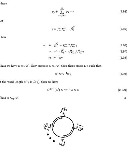
5.4 Translation from Conway’s K n o t a t i o n ... 110
6 T h e S olar H e a tin g P r o b le m 112 6.1 In tro d u c tio n ... 112
6.2 The Tem perate P h o to sp h e re ... 116
6.3 Generating Arches from F o o tp o in ts ... 117
6.4 The S im u la tio n ... 117
6.5 M utual and Self H e lic ity ... 118
6 . 6 The Moving Footpoints ... 120
List o f F igu res
1.1 The unknot, Hopf link and W hitehead link ... 16
1 . 2 The Reidem eister m o v e s ... 17
1.3 The 3 -sim p lex ... 19
1.4 Longitude and m e r i d i a n ... 2 0 1.5 Two forms of double p o i n t s ... 2 1 1.6 Canonical closure of a b r a i d ... 23
1.7 P lait closure of a b r a i d ... 23
1 . 8 The generators of the braid g r o u p s ... 24
1.9 The Markov m o v e s ... 27
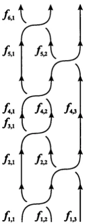
2.1 The braid A3 la b e le d ... 35
2.2 The braid A3 la b e le d ... 37
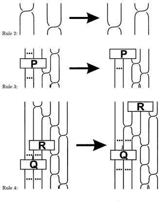
2.3 The rules for th e word p r o b l e m ... 43
2.4 Cyclic words i l l u s t r a t e d ... 47
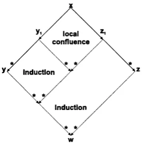
2.5 P roof of N ew m an’s L e m m a ... 49
2.6 P roof of cyclic critical pair lem m a ... 56
4.1 Reduction r a t i o s ... 87
4.2 Exam ple reductions of all m e t h o d s ... 89
4.3 Energy com parison of reduction m ethods ... 90
5.1 3-ball ... 93
5.2 Elem entary t a n g l e s ... 93
5.3 Tangle a d d i t i o n ... 94
5.4 The universal p o l y h e d r o n ... 96
5.5 The trefoil knot l a b e l e d ... 97
5.6 The trefoil knot in P ( 2 , 2 ) ... 98
5.7 K not a d d itio n ... 1 0 0 5.8 An axis for th e trefoil knot ... 103
5.9 The trefoil knot around its a x i s ... 104
L IST O F F IG U R E S ___________________________________________________________________ 8
5.11 The conversion of a knot into a p l a i t ... 106
5.12 The braiding a x i s ... 107
6 .1 The solar c o r o n a ... 113
6 . 2 Flux tubes in the c o r o n a ... 114
6.3 Loop p ro m in e n c e ... 114
6.4 Schematic flux tu b e m o d e l... 116
6.5 The com puter m o d e l ... 118
6 . 6 The helicity angles d e fln e d ... 119
List o f Tables
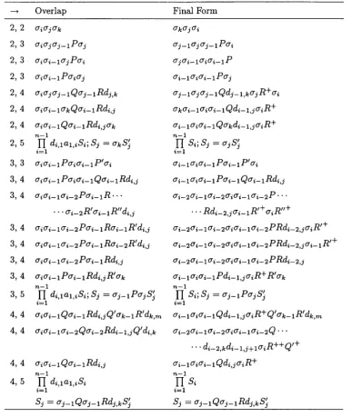
2.1 Overlaps between rules in the word problem s o l u tio n ... 45 2.2 Cyclic overlaps between rules in W n... 52
3.1 The Size of Diagrams of Fundam ental W o r d s ... 71
4.1 Reduction ratios a = Cmin/C{Qi) as a function of th e num ber of strings n ... 8 6
N o ta tio n
The m ost im portant symbols used throughout the thesis are explained in the table below.
Symbol Meaning
[A,B] A B - B A = 0
ai generator of braid group, single braid crossing
Bn braid group of n strings
% equivalence in a group
conjugate in a group
Markov equivalence in braid group
L{A) num ber of A rtin generators in braid A; the length of braid A
A (canonical) closure of b raid A
fundam ental group of com plem ent of knot K p{K ) peripheral group system of complem ent of knot K (^i,j = • - aj for i < j ascending braid word
di,j = aiUi^i • ■ - aj for j < i descending braid word An = <%i,n-iai,M- 2 • • • fli.i fundam ental braid, see
A cknow ledgem ents
B ody and soul m ust be kept together while doing m athem atics. My gratitude goes to the G raduate School of University College London which has kindly provided this param ount service through awarding me a research scholarship. I am indebted to Mitchell A. Berger, my supervisor, for taking me on, supporting me through my learning and researching, and reading the drafts of papers and thesis while m aking m any helpful comments and suggestions th a t lead to new and exiting things.
T hanks go to M argaret Yoder for providing insights into her thesis and into rew riting systems, to Claude M arche and Benjam in M onate for all their help, explanations and patience and for the provision of th eir excellent term rew riting software CiME w ith which m any ideas were tested during the development of the rewriting systems, to Mike S. P aterson for explanations of his work w ith Alexander A. Razborov and John M. T albot for excellent explanations of complexity theory. M any other m athem aticians helped me during the developm ent of this work and the associated software program BraidLink.
P reface
This thesis considers several problems in the theory of braids. B raid theory is a branch of knot theory which is contained w ithin topology. During the discussion of the research, we make use of braid, knot, group and tangle theories as well as techniques from term rew riting systems and NP- completeness which come from com puter science, and topology. O ther th a n a basic knowledge of topology and group theory, no further knowledge of any other branch of m athem atics or com puter science is necessary in order to read this thesis as we review all these fields to the extent necessary for our purposes.
We begin in chapter 1 by reviewing braid and knot theory. In section 2.1, we use group theory
and algebra to deduce certain properties of the braid groups. We proceed in section 2.2 to review term rew riting system s and use them in section 2.3 to solve th e word and conjugacy problem s in the braid groups.
We state the m inim um word problem for braids in chapter 3. In section 3.2, we review the theory of NP-completeness and use it to show th a t th e m inim um word problem is NP-com plete in section 3.3. We find, in section 3.4, an algorithm to solve th e problem which runs in exponential time.
The m inim um word problem may be approached by sim ulating braids as elastic strings. This approach works well in practice. In section 4.2, we discuss how to generate a random braid, embed it in space and retrieve a braid word from a set of strings. In sections 4.3 and 4.4, we present three forces th a t we will use in the simulation. Section 4.5 presents an efficient algebraic heuristic algorithm to solve th e problem. The properties of th e forces and d a ta to compare them in b oth efficacy and efficiency is in section 4.6. The sim ulation contained in chapter 4 was published in a slightly different form in [1 0].
We review tangle theory in section 5.1. Section 5.2 presents a new notation for knots and gives a few basic properties of it. We solve the problem of turning a knot into a braid or plat in section 5.3 and give translation algorithm s between our new notatio n and existing com puter notations in section 5.4.
13
reasons of space we provide the proof of a result only when it or th e result is new and refer th e reader to the literatu re if th e proof exists therein.
In the investigations described in the above chapters, com puter assistance was frequently nec essary and for this purpose a program called B raidLink was w ritten in C+-f- for M icrosoft W in dows. Many of th e algorithm s in this thesis are im plemented in B raidLink b u t the functionality of BraidLink goes far beyond them . The program m ay be obtained from the author, for further inform ation and th e m anual see h t tp :// w w w .k n o t - th e o r y .o r g .
For each entry in th e bibliography, we provide a list of page num bers on which th a t p articular work was cited. A fter th e bibliography, we provide an index to the technical term s used in the thesis. Page num bers in bold indicate th a t th e term is defined on th a t page whereas a norm al page num ber simply m eans th a t the term is used in an im portant way on th a t page.
C hapter 1
In trod u ction to B raid and K not
T h eory
1.1
K not T heory
Everyone has encountered knots. We use knots to tie our shoelaces, fasten our washing lines and secure ourselves from falling during climbing. K not theory studies th e topology of knots such as these with th e only additional requirem ent th a t after they are tied, the ends m ust be glued together never again to be undone. The inherent freedom of topology means th a t we are allowed to do anything to th e knot - stretch, bend, tw ist and d isto rt it in any way - except cut or glue the string a t any point. The m odern view of thinking of a knot as a tied piece of string w ith connected ends is much simpler th an the original conception:
” By a knot of n crossings, I understand a reticulation of any num ber of meshes of two or more edges, whose sum m its, all tessaraces (a/tT?), are each a single crossing, as when you cross your forefingers straight or slightly curved, so as not to link them , and such meshes th a t every thread is either seen, when th e projection of the knot w ith its n crossings and no more is draw n in double lines, or conceived by the reader of its course when draw n in single line, to pass alternately under and over the th rea d s to which it comes a t successive crossings.” [93]
In tr o d u c tio n to B ra id and K n o t T h e o r y 16
to produce a theory of everything. The 1887 experim ent of Michelson and M orley showed th a t th e luminiferous ether does not exist and thus th e vortex atom theory was abandoned. However knot theory continued as a m athem atical discipline. T ait was prim arily concerned w ith creating a table of topologically distinct knots in order of increasing complexity. The m easure of complexity used was the minimum number of crossings over all two dimensional projections of the knot. Tait succeeded in creating a rem arkably accurate table of prim e knots up to and including ten crossings.
Figure 1.1: The unknot, Hopf link and the W hitehead link. These knots are oriented as indicated by th e arrows. K nots do not have to be oriented b u t every knot is orientable and different orientations m ay not be deformable into each other w ithout cutting or gluing, i.e. they m ay be topologically distinct.
Figure 1 .1 gives three examples of knots. T he leftm ost knot is called th e unknot and was
originally not regarded as a knot a t all. T he unknot is a very special case and arguably the most im portant single knot. The other two are the Hopf and W hitehead links respectively which have two closed loops of string each. The term link is usually reserved for a knot w ith more th a n one component. The arrows on the diagram s supply an orientation to th e knot. The orientation is im portant because there exist knots for which altering th e orientation can change the topology. M any tim es however, no orientation is specified.
T he m odern definition of a knot K is an em bedding of n copies of into 5^, the three-sphere (thus we use the term knot as inclusive of links). W henever a new m athem atical object is defined, th e question arises how equality is to be defined. In knot theory this is far from obvious and there were several contending views very early on. T ait [142] viewed knots based on string and allowed axial tw isting of the rope while K irkm an [93] viewed knots based on ribbons and did not allow axial tw ists. This lead to different tables of distinct knot types and created some confusion.
T he definition of equivalence is based on th e topological concept of am bient isotopy and is essentially the same definition th a t T ait used. Two embeddings fci, /c2 : X —> Y are ambient
isotopic, denoted by %, if there is a level preserving isotopy H such th a t
H : Y X I X I , H { y , t ) = {ht{y),t) (1.1) where ^ 2 = ^ i^ i, ho = id y and / = [0,1]. H is called th e ambient isotopy. This m eans th a t if
1.1 K n o t T h e o ry 17
both th e same knot. If we m ust go through some discontinuities, i.e. if we m ust cut or glue, then the two are not the same knot. From this definition, it is clear th a t the unknot and th e Hopf link in figure 1.1 are not the same knot. The reason is th a t th e H opf link has two com ponents which could be reached from the un k n o t’s single com ponent only by cutting and gluing. This process of cutting and gluing is commonly referred to as surgery.
Having defined w hat it means for a knot to be equal to another, we ask for a m ethod to discover if the equality holds between any two given knots. This is the classification problem for knot theory and no satisfactory answer has yet been given.
1.1.1
T h e K n ot C lassification P rob lem
Figure 1.2: The Reidemeister moves.
The overriding problem in constructing a knot table is th e difficulty of determ ining w hether two knot diagrams are topologically distinct or not. It is possible to construct all possible knot diagram s up to a given number of crossings using an (essentially) algebraic m ethod [143] bu t distinguishing these is the real problem. This enum eration m ethod has been refined [58] and used to tab u late knots based on topological invariants (see below) up to and including 17 crossings [69] (for an excellent review on the history of tab u latio n and how it is done using a com puter see [147]). Therefore a practical m ethod for com paring two given knot diagram s would make it possible to construct a complete knot table up to a certain num ber of crossings, i.e. such a m ethod would classify knots. After Tait, Reidemeister [130] showed th a t two knot diagram s are equivalent if and only if they can be transform ed into each other via a set of four moves which are called Reidemeister moves, see figure 1.2. W hile this tu rn s th e problem into a com binatorial one, it is often necessary to further complicate a diagram in order to fully simplify it later. M aking this transform ation is not readily am enable to algorithm ic m anipulation. T hus R eidem eister’s moves do not present a practical m ethod to distinguish knots. They make it easy however, to prove the invariance of other properties of knots. If one can show th a t a p articular function / (K ) calculated firom a knot K is invariant under all the Reidem eister moves, then / (K ) is a topological invariant
In tr o d u c tio n to B ra id an d K n o t T h e o r y 18
of knots. This m eans th a t if K i % Kg, th en / ( K i ) = / (Kg). M any such functions have been found b u t it can be shown th a t for m ost known functions it does not follow th a t if / ( K i) = / (Kg), th en K i ~ Kg. In th a t sense, m ost topological invariants are incomplete. An invariant is called complete when K% % Kg if and only if / ( K i ) = / (Kg). It is the holy grail of knot theory to find a (readily com putable) complete invariant. It is not known w hether such an invariant actually exists. As we will discuss below, th e complement {R^ w ith the knot removed) of the knot is a complete invariant b u t distinguishing these, while possible, is such a tim e consuming affair, th a t this m ethod of classifying knots is not practical [77].
We can define a knot sum K i# K g between two knots K \ and Kg by cutting both knots a t one arb itra ry point and splicing th e ends together in such a way th a t th e orientations, if any, are compatible. It can be shown th a t this sum is independent of the choice of th e points and thus dependent only upon which com ponents of K \ and Kg are cut [39]. It can also be shown th a t there is no inverse to this sum, th a t is, in general, there is no knot K ~ ^ for any knot K such th a t K # K " ^ % U where U is the unknot of as m any com ponents as K has [39]. Therefore, the knot isotopy problem does not reduce to recognizing the unknot, which is a fundam ental complication of th e problem. A knot is called prime if it can no t be represented as the sum of two non-trivial knots, it is called composite otherwise.
1.1.2
T opological Invariants
The topological invariants of knots fall into a num ber of categories. A trivial invariant is the num ber of com ponents b u t since there are a large num ber of obviously distinct knots for each value, this is not a very strong invariant even though it is easily com putable. Am ongst th e simplest to state are th e invariants which are defined as the m inim um of quantities over all possible diagram s of a knot. Since there are an infinite num ber of diagram s for each knot, these invariants are difficult to determ ine and for m any of them , there exists no general m ethod. Exam ples of this are the minim um crossing num ber, bridge num ber and braid index [116]. A nother im portant category is formed by the polynomial invariants. A num ber of polynomials have been defined which are topological invariants of a knot. The polynom ial is generally calculated via a topological form of recursion relation, called a ’’skein relation,” which we will not go into [91]. T he Jones polynomial and its generalization, th e Homfly polynomial, are very im portant in several applications of knot theory as well as knot theory itself. They are very powerful invariants b u t there are still an infinite num ber of knots w ith identical polynomials. The fundam ental point to note is th a t, while polynomial invariants are among th e m ost powerful knot invariants, the am ount of com puting tim e required to determ ine them increases exponentially w ith the num ber of crossings in th e diagram of the knot. For a review on knot polynomials, see [99].
1.1 K n o t T h e o r y 19
question is negatively resolved, th en the Jones polynomial would provide the best known unknot detection m echanism (from a com putational point of view) [21]. There are two algorithm s which can distinguish th e unknot: One due to Haken [74] [75] which was th e precursor to his classification of 3-manifolds and one due to B irm an and Hirsch [2 1] which makes use of closed braids. While the
former is clearly exponential in execution tim e, the later has not been analyzed for complexity bu t appears to be exponential. It has not been analyzed w hat the com plexity of th e knot classification problem in general is b u t it would seem to be easier to distinguish a knot from th e unknot th a n to distinguish two a rb itra ry knots.
1.1.3
T h e C om p lem en t o f th e K n ot
We define a knot K as an em bedding of n copies of into 5^, the three-sphere. Consider the knot K and surround it w ith a tu b u lar neighborhood V { K ) , th en the manifold C { K ) = — V { K ) will be called th e complement of K . It can be shown th a t for any knots K \ and K2, K \ % K2 if and only if there exists orientation preserving homeomorphism H : C { K i) —> C {K2) [39]. Thus the knot com plem ent is a complete invariant of th e knot.
P,
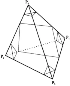
Figure 1.3: The stan d ard 3-simplex or tetrahedron.
C { K ) is clearly a 3-manifold and it can thus be distinguished (or otherwise) from other 3- manifolds, in particular other knot complements C {K '), by H aken's classification of 3-manifolds. We briefly present th e idea of th e m ethod b u t refer the reader to [77] for a pedagogical treatm ent. F irst, a triangulation m ust be found on R^. A triangulation for a 3-manifold essentially consists of filling th e manifold w ith non-overlapping te tra h e d ra in such a way th a t any point in the manifold is in a tetrah ed ro n , see figure 1.3. Any surface in the manifold will now intersect some tetrahedra. These intersections will be triangles (2-simplices) or squares, see figure 1.3. Since the tetra h ed ra do not overlap b u t fill all of th e manifold, the num ber of intersections of a surface w ith adjacent sides of te tra h e d ra m ust be equal. This requirem ent gives a set of equations describing th e surface in the manifold. Since the triangulation is not unique, neither is the set of equations. Com paring two knot complements has been a topological problem b u t this construction tu rn ed it into a com binatorial
I n tr o d u c tio n t o B ra id an d K n o t T h e o r y 20
one. If we can compare th e set of equations from two surfaces (thickened knot neighborhoods of K and K ') , then we can distinguish th e knots. This can be done [77] b u t the time taken is exponential in the num ber of crossings of the knot, so exponential th a t the algorithm can not be used to practically distinguish knots even of small crossing number.
1.1.4
Peripheral G roup S y stem
T he complement of a knot is uniquely specified (up to isomorphism) by its peripheral group system which consists of the fundam ental group and a few subgroups thereof (this is W aldhausen’s theorem [153], see [78] for a m ore accessible proof). This is the only com plete invariant which it is practical to actually calculate b u t since group isomorphism is algorithm ically untestable (the Adian-Rabin theorem [2] [3] [129]), this does not provide a practical m ethod to distinguish knots either. It is however known th a t th e word problem for any fundam ental group of any knot is solvable [154]. If th e knot is alternating, th e conjugacy problem is also solvable [5].
Figure 1.4: The thick curve displays the trefoil knot w ith an orientation. The th in curve which is parallel to the trefoil knot is the longitude; th e orientation of the longitude is th e same as the knot. T he th in curve encircling both trefoil and longitude a t the top left hand corner is the meridian. N ote th a t the five conditions given in the te x t are fulfilled by these curves.
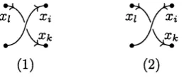
We define the linking number of two curves a and 6, denoted by lk{a, b) as the weighted sum
of th e characteristics e of each crossing. T he characteristic e is - 1 or 1 depending on w hether the crossing m atches respectively w ith the first or second of the two possible scenarios for a crossing shown in figure 1.5. We define a meridian m i and a longitude U of a knot component K i by requiring the following properties: {!) rui and li are oriented, polygonal, simple and closed curves in d V (Ki), the boundary of the thickened neighborhood of K i which we denote by V (Ki), (2) rUi and U intersect in exactly one point, (3) rUi is null homologous (m^ ~ 0) in V {KÎ) and U ~ K i in V (K i), (4) /i ~ 0 in C (K i) and (5) l k ( m i , K i ) —1 and l k ( l i , K i ) = 0 in S^. The above five
properties define nrii and U uniquely up to isotopy on the boundary of V ( K ) [39] (see figure 1.4 for an illustration). The meridian-longitude system pair A i ( K ) for a j-com ponent knot K is the pair of sets ({m i, m2, - - - ,m j} , {/i,Z2, • • • ,lj} ).
1.2 K n o t N o ta tio n s 21
m ay be considered to be elements of 7t(K ) by choosing a p ath pi in C { K ) from the base point b to
th e (unique by definition) point rrii fl k for each i. Then the subgroup (rriiji) of tv{K), generated by rrii and h is independent of th e choice of pi up to conjugation. T he peripheral group system of a ^-com ponent knot K is p{K ) = {'k{K)\M .{K)). By an isom orphism (j) between two peripheral group systems p {K) p {K'), we m ean tf {K) % tf {K') such th a t (f) {rrii) = and (f> {k) = I'i for all i. It can be shown th a t for any two knots K \ and K2, p { K \ ) % p (K2) if and only if K \ % K2 [92]. If we restrict attention to prim e knots of a single com ponent, we have t t { K i ) % tt (K2) if
and only if K i ^ K2 [92]. Thus the problem of knot isotopy can be transform ed into the problem of peripheral group system isomorphism. Since it is not possible to determ ine, in general, if two groups are isomorphic, this does not solve the knot classification problem.
( 1) (2)
Figure 1.5: The two possible forms of double points in the diagram of an oriented knot.
There exists a simple m ethod due to W irtinger, to find a presentation of tt{K ) from a diagram of K . Suppose there are n arcs in th e diagram . We label th e arc by Xi. The set for 1 < i < n generates tt{K). Every crossing in th e diagram of K is of one of th e two kinds displayed in figure 1.5. For each crossing determ ine its type and add the relation xiXiX'j^^ x~^ w e or xixJ^x'j^^Xi w e to the group respectively. The resulting group is 7f(K ) defined by its Wirtinger presentation. It
is a practical observation th a t this presentation can often be simplified considerably in th a t some generators are removable [65]. In particular, r { K ) for the torus knot Tp,g, which is a knot th a t winds around a torus p times th e short way around (meridionally) and q tim es th e long way around (longitudinally), is given by r { K ) = ({n, 6} : a^ = b^) [92].
Even though r { K ) can not be readily used as a practical invariant, it is however a convienient sta rtin g point to define m any other invariants, for example the A lexander polynom ial [148] which was th e first of the polynomial invariants and (like the Jones polynom ial) revolutionized knot theory.
1.2
K not N otation s
K n o t theory has gained trem endous m om entum from proofs th a t certain m athem atical objects are isotopy invariants of knots such as the peripheral group system discussed above. Such proofs and general statem ents about knots form a large p a rt of knot theory b u t in applications of knot theory, actual com putation of these objects is often necessary. Therefore, it is im portant to have a practical m ethod of com putation for such invariants. Some invariants, such as the unknotting
I n tr o d u c tio n to B ra id an d K n o t T h e o r y 22
num ber, can not yet be calculated in an algorithm ic m anner for every knot. O ther invariants can only be calculated by algorithm s whose complexity increases exponentially, thus rendering them useless for all b u t small knots. There exist only a few invariants which m ay be calculated easily.
Because it is so laborious to com pute m any interesting properties of a particular knot, the use of com puters is essential. However if a com puter is to be used, th e search for an efficient algorithm becomes im portant. T he pivot of all algorithm s is th e form of th e input. For m any physics calculations, for example, th e choice of coordinate system often allows far greater simplification of the calculations th a n a change in com putational procedure. Therefore, while the algorithm is im p o rtan t, a good notation for knots is param ount. C urrently there are several different systems of ’’kn o tatio n ” (the term was coined by John Conway in a popular lecture w ith this title) which are widely used, we shall illustrate two of them : Conway’s [50] and Dowker and T histlethw aite’s [58],
Conway’s knotation relies on setting up tem plates for knots which he calls basic polyhedra. One inserts stan d ard knot pieces called tangles into the vertices of th e tem plate (tangles are introduced in chapter 5). T his knotation is quite intuitive since th e geom etrical aspects of the knot projection can be im m ediately visualized it is however non-trivial to construct the notation given a knot projection and the notation is limited to knots w ith few crossings w ithout making necessary extensions.
T he Dow ker-Thistlethw aite code for a knot is an im provem ent of T a it’s notation. One chooses a point on th e knot a t random and follows it in the direction of its orientation. The crossings are nam ed ”A ” , ”B ” , ” C” and so on in the order th a t they are m et and one writes down which ones one m eets in order. It can be shown th a t only every second letter is needed as the others can be recovered and so the notation for a knot projection of n crossings contains n letters. Im plem ented algorithm s to calculate m ost invariants from this code exist. The m ain application of this code is in th e com puter-assisted tab u latio n of knots [147]. In chapter 5, we introduce a new notation which will allow us to transform a knot into a closed braid (see next section).
1.3
B raid T heory
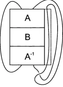
In 1923, A lexander proved th a t any knot projection can be modified via Reidemeister moves into a form w ith respect to a special point P in the plane which has the property th a t for a point A which traverses the knot in th e direction of its orientation, a plane perpendicular to th a t of the projection intersecting b o th P and A rotates around P in a constant direction (clockwise or anti clockwise b u t never both) [4]. W hen A rtin invented braids [7], it was noticed th a t if one specified a point outside th e braid to be P and connected the to p and bottom ends of th e b raid ’s strings w ith each other in such a way th a t th e connecting lines circum navigated P (this process is called closing a braid, illustrated in figure 1.6) and oriented th e b raid ’s strings in a uniform (upwards or
1 .3 B ra id T h eo ry 23
Figure 1.6: The (canonical) closure of a braid. In th e braid group language, the braid is A3
0-1(72(71 and the knot is the Hopf link.
Figure 1.7: The plait closure of a braid. Note th a t there is potential conflict between orientations of the braid strings in the plait closure; it becomes impossible to plait a braid in which all strings are oriented in the same way.
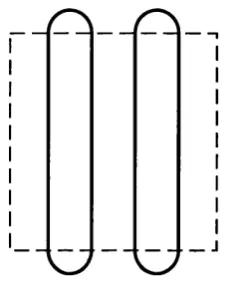
(oriented) knot can be represented by a closed (oriented) braid. In his paper, A rtin had found a group structure for braids which defined open braid isotopy - th a t is topological equivalence of two braids under the restriction th a t th e endpoints rem ain fixed. The m ethod of closing a braid which is illustrated in figure 1 .6 is called the canonical closure to distinguish it from the plait closure. In
th e plait closure, we join neighboring ends together as illustrated in figure 1.7. It is necessary for the braid to have an even num ber of strings for the plait closure.
1.3.1
T he Braid G roup
T he braid group Bn for a braid of n strings is generated by single crossings. Suppose th a t all strings are vertical ap art from strings i and i + 1 which cross over each other. If i overcrosses z + 1 , we denote this by ct* and the inverse is denoted by ct~^ (see figure 1.8 for an illustration). The set {(7 1,(7 2, • • • , (7n-i} generates th e group Bn and together w ith their inverses {(7j“^ , • • • ,
I n tr o d u c tio n to B ra id a n d K n o t T h e o ry 24
Bn satisfies the defining relations (7iCT^
(Ji(Tj Giai^iOi
e
(jjai for \i — j\ > 1 O’i+lO'iO’i+i
(1.2)
(1.3) (1.4)
where e denotes th e identity element. Topologically e is the braid of n strings w ithout any crossings; i.e. n vertical strings. T he generators cr^ are called A rtin generators. T he proof th a t the topological equivalence relation of braids is identical to th e group theoretical equivalence relation defined by the equations above under th e m ap th a t a crossing in the topological braid is interpreted as a generator in th e group is given in [8] or more accessibly in [39]. We shall use ~ to denote equivalence under
a given set of identities and = to denote exact (letter by letter) equivalence.
1-7
CT.-1
i+ 2 n-1 n
i-1 i+ 1 i+ 2
Figure 1.8: T he generator and its inverse ^ for th e braid group Bn-n -I n
We will call a word positive if it contains only generators and no inverses; the inverse of a positive word is called negative. We shall call two positive braids A and B positively equal if there exists a sequence of braids Wi ioT 0 < i < q w ith Wq = A, Wg = B , W j and different by a single application of th e b raid group’s defining relations and Wi all positive. Garside has shown th a t if two positive braids are equal, they are positively equal [64].
T he length of braid A in term s of A rtin generators will be denoted by L{A). A general braid A E B n may be w ritten in th e form
Jl( A )
iL{A) (1.5)
where 1 < < n and jk = ± 1 for any k : 1 < k < L{A). We define th e exponent sum, denoted exp (A) of A by
L ( A )
exp(A) = ^ jk fc=i
(1.6)
I t can be shown th a t exp (A) is a conjugacy class invariant (and hence equivalence class invariant) of A [2 0]. If A is as in equation (1.5), then we define the reverse operator R by
1.3 B ra id T h e o r y 25
and call R {A ), th e reverse of A.
We define three special braid words: The fundamental braid A „, th e ascending braid a i j and th e descending braid d i j by
^i,j ~ ■ ■ ' ^ j ‘I — j (1 8 )
di^j — • • ■<7j j i (1 9 )
A n = a i a 2 • • ■ CTn-lCria2 • ' - (Jn -2 ’ ’ ’ (1.10)
~ Ûl,n—l^l^n—2 ■ ■ ■ ®1,2<^1,1 (1 11)
An is im p o rtan t in b raid theory because A^ generates the center of the braid group B n [43]. Garside [64] has shown th a t th e fundam ental braid satisfies
An<7i ~ (Tn—i ^ n ~ (1 1 2)
A (An) % An (1.13)
where we have defined Oi = (Tn-i- We now prove a crucial proposition. P r o p o s i ti o n 1.3 .1 For any ct~^, we have <j~^ % A ” ^ A n - id n - i,i+ id i_ i,i. P r o o f . Since A „ = a i ,n - i a i ,n- 2 • • • 0 1,2^1,1 and iî( A n ) ~ A n, we have A „^ ? T hus d n -1,1 ~ 1^2,1 • • • d n -2,1- From the definition of d i j , we have
^ ~ a i - i a i - 2 " - ( ^ i d n ^ i iCrn-iO'n-2---cri+i (1.14)
~ di—l,ld^_-^ldn-l,i+l (1.15)
~ d i _ l , l A “ ^ d l , 1^2,1 • • • d n - 2 , l d n - l , i + l (1.16)
~ A “ ^ a n - z + l , n - l d l , l d2, l • • • d n - 2 , l d n - l , i + l (1.17)
^ A n rin—i + l , n —1 A n —i d n —l , i + l (1.18)
~ A n A n —i d j —i ^ i d n — (1.19)
~ A n A n —i d n — (1.20)
for any i, which proves th e proposition. □
Given two words ct,P E Bn, the decision problem of w hether o % is called the word problem. T he word problem in th e b raid groups was first solved by A rtin [8] and therefore provided a solution to th e problem of braid isotopy. For two words a, (3 E B n, if th ere exists a word j E Bn such th a t a % 7/3 7“ ^ then a and /? are called conjugate, which is denoted by «c- If 7 ~ e, then a P implies a ^ P and th u s th e conjugacy problem, the existence decision of such a 7, contains the word problem as a special case. T he conjugacy problem for B n was first solved by Garside [64]. T he best known algorithm for the word problem was form ulated by B irm an, Ko and Lee [2 2] w ith com plexity O (nL^), where L denotes word length, and for th e conjugacy problem by T hurston [59] and B irm an, Ko and Lee [2 2] w ith exponential complexity.
In tr o d u c tio n to B ra id an d K n o t T h e o r y 26
C onstruct the set D{A) of all words obtainable from A by rearranging of generators, this is called the Cayley diagram of A. This set is constructed recursively from A. The first set is Do(v4) = {A} and each set D i{A) is obtained from D i - \ { A ) by adding all words which can be obtained from the members of D i - i { A ) by a single application of th e relations 1.3 and 1.4 and are not already members of the sets D j{A ) for 0 < j < i. It is a theorem of Garside [64] th a t this construction process term inates in a set Dk{A) for finite k and th a t thence th e set D {A) which is th e union of all the Di{A) for 0 < i < fc is finite and readily constructible. Since we do no t allow cancelations or introductions of generators by use of th e relation 1.2, it is an obvious p roperty of
D {A ) th a t all members are of equal length L{A).
For any two braids A, B G B n we say th a t A is prime to B if and only if D {A) does not contain a word in the form A % A \ B A2- Let the num ber of inverse generators in a braid A be s(v4), then proposition 1.3.1 together w ith equation (1.1 2) implies th a t any braid A € Bn may be w ritten in th e form Amax — An^^^^^A' where A is positive; the reason for nam ing it Amax will become apparent later on. We obtain this form by replacing each inverse generator in A by the form given in proposition 1.3.1 and then using equation (1.12) to bring all th e fundam ental braids to th e front.
In his celebrated solution to the word and conjugacy problem s in B ^ Garside [64] presents an algorithm to put A ' into the form A ' = A ^ A " where A!' is prim e to and another algorithm to p u t A!' into a form minimal in lexicographical order on th e set of generators for the ordering Ui < Uj if and only if i < j , which we call A. Garside shows th a t the resulting form Ag = for the braid A is unique. We call q — s{A) the Garside exponent and A the Garside remainder of th e braid A. G arside’s original algorithm s have exponential complexities in n and L{A), however Jacquem ard constructed an algorithm with complexity 0 (n^L (A )^) [83].
In stating the complexities of all algorithm s here, we im plicitly assume th a t n and L {A) are independent. Clearly, we m ay choose a braid A G B n of any length at all and thus it would appear th a t we are justified in this assumption. In th e class of non-splittable braids (A braid A G Bn+m is said to be splittable if and only if it m ay be w ritten in the form A % aOn{P) where a G Bn, P € Bm and the operator 0 „ is defined by 0 „(oTi) = [2 0]) this is not true as we m ust
have L{A) > n — 1. As in th e case of worst-case complexity m easurem ents, we are interested in th e asym ptotic behavior as n and L{A) —^ oo, we m ay continue to assum e th a t n and L (A ) are independent. Should this in some circum stances tu rn out to be false, th e above argum ent shows th a t th en n is of the order of L{A).
If a knot K is represented by a closed n-braid /?, th en the m irror image K * of K is represented by the closed braid and th e reverse (obtained by reversing th e orientations) of K is represented by R{P) or by R { P y [117].
We will henceforth represent a com m utation relation A B = B A by w riting [A, B ]. P u t a = û i,n - i and /? = <Ti, then it can be shown th a t another presentation of the braid group is [51]
1.3 B raid T h e o r y 27
where a " is the generator of th e center Z (B „) [43]. In this formulation we trivially find the following helpful simplifications
a ^ (1.2 2)
r ' (1.23)
= « - ’',9 (0 /))’'- ^ a (1.24)
(1.25)
1.3.2
M arkov’s T h eorem
Given a knot, we m ay produce an equivalent knot by taking any segment and tw isting it about an axis in the projection plane by tt while keeping the rest of the knot stationary. This procedure corresponds to the zeroth Reidem eister move (see figure 1.2) and adds one crossing to the diagram . Any crossing of this ty p e is called nugatory. If we represent a knot by a closed braid by virtue of A lexander’s theorem , we m ay also add such nugatory crossings via a com binatorial move, called the Markov or stabilization move (see figure 1.9). Stabilizing a braid a e Bn corresponds to the operation a —> cx.(j^^ or its inverse. Clearly stabilization increases or decreases the num ber of strings in the braid and so represents a move in the family of braid groups as opposed to the conjugacy and equivalence moves which are contained in a single braid group.
Figure 1.9: B oth conjugacy and stabihzation are displayed here. We begin w ith braid B . Con jugation surrounds B w ith A and A~^ on opposite sides which clearly cancel due to th e closure. Stabilization introduces a simple loop at the bottom right of th e braid, adds a new string to the braid and thus increases th e braid group index by one.
Markov stated in 1935 [105] th a t two closed braids are topologically equivalent if and only if they differ by stabihzation and conjugacy moves (recall th a t conjugacy contains equivalence). This statem ent became known as M arkov’s theorem and was first proven in [20]. In its original form, M arkov’s theorem assumes th a t the closed braid is em bedded in or this can however, be generalized to an arb itra ry 3-manifold [97]. M arkov’s theorem transform s the link isotopy problem
In tr o d u c tio n t o B r a id a n d K n o t T h e o ry 28
to a com binatorial question about braids. If two braids a E Bn and j3 G Bm (with n and m possibly different) are related by stabilization and conjugacy, they are called M arkov equivalent which is denoted by « m - T h e decision problem of w hether a « m P is called the Markov problem or the algebraic link problem. It is possible to find a single move of which both stabilization and conjugacy are special cases and to formulate, in this way, M arkov equivalence in term s of this so called L-move [98]. W hile this L-move is intuitive, it is not obvious w hether the problem has been simplified by this reform ulation.
1.3.3
S ta b iliza tio n is N on -trivial
The first question which arises is w hether there exist non-conjugate Markov equivalent braid words in the same braid group, th a t is w hether a solution to the conjugacy problem will solve th e M arkov problem. T his is negatively resolved by showing th a t the two 4-braids a = ctj and = aY^a^o-i w ith m , n , p different, odd and a t least three in absolute value are not conjugate b u t M arkov equivalent [118]. It m ight be thought th a t it should be possible to reduce th e num ber of strings in a closed b raid equivalent of the unknot to one. This is tru e as all equivalent closed braids can be reached from each other via M arkov’s theorem b u t the transition involves, in general, increasing th e num ber of strings before they m ay be reduced to a single string. In other words, a greedy reduction of strings does not reach the m inimum string num ber, also known as th e braid index (not even for th e unknot representatives) [114].
It is a practical observation th a t finding a series of moves to dem onstrate the Markov equivalence of two closed braids is very difficult. The difficulty of finding such a sequence has lead B irm an to believe th a t it m ay be simpler to solve M arkov equivalence for two braids representing prim e knots. W hile this m ay be tru e, it is not, in general, easy to decide w hether a braid represents a prime knot. Schubert [132] proved th a t the factorization sequence of a composite knot is unique and has found an algorithm [133] which finds it. This algorithm , consequently, is able to decide w hether a knot is prime. However, the execution of th e algorithm rests on Hemion’s algorithm since it m ust identify th e prim e factors of the knot, thus no longer necessitating a solution of the Markov problem since it already solves the fink isotopy problem (albeit im practically so). This also shows th a t this m ethod of deciding prim ality is not practical. B irm an conjectures th a t a braid represents a prim e knot if and only if it is not conjugate to a split braid.
1.3 B ra id T h e o r y 29
1.3.4 S trategies for th e M arkov P rob lem
Since the word and conjugacy problems are contained in the Markov problem, solutions for these are desirable and have been given numerous times as m entioned before. The stabilization move represents the final hurdle before link isotopy is algorithm ically decidable and thus it would be interesting to know when a braid a G Bn+i is conjugate to a braid where 7 contains only the
generators cr^ for 1 < i < n — 1, for then one could reduce A to 7 using the Markov move. While
this has been done [107], th e algorithm depends on G arside’s conjugacy algorithm [64] which has exponential complexity. Moreover, if two braids were reduced in this way to th e minimum string num ber, they are not, in general, conjugate in this final braid group if they are M arkov equivalent and thus this decision procedure does not solve th e M arkov problem either.
We have defined th e exponent sum exp{a) of a braid a as the sum of the exponents of the A rtin generators of a . It is obvious th a t the exponent sum is a conjugacy class invariant b u t not a Markov class invariant because of stabilization. T hus it is possible for two braids to be Markov equivalent and have different exponent sums. In getting from one braid to the other, the exponent sum m ust be made equal somewhere in the chain of moves; this can clearly only be accomplished using stabilization. Stabilization can increase or decrease the exponent sum depending w hether we add (Tn or or remove either of these. It also changes the num ber of strings. We m ay think th a t startin g from a positive braid, we should be able to reach any M arkov equivalent positive braid by going through a pure positive sequence of braids; th a t is, we m ay think th a t positive Markov equal braids are positively Markov equal. We note th a t this would only be possible if the difference in exponent sum between the two braids was precisely their difference in num ber of strings. We conjecture th a t positive M arkov equal braids are no t positively Markov equal.
Much work was done by B irm an and Menasco on various properties of links which could be determ ined from their closed braid representatives (this work was published in the six-paper series [23], [24], [25], [26], [27] and [28]). They prove th a t there exists a complete num erical invariant for knots bu t find this invariant only for knots which are closed 3-braids. The invariant for closed 3-braids is described extensively and can be used to determ ine the braid index and w hether the knot is spht, composite, amphicheiral or invertible. T hey also define a new type of move on braids, the exchange move, and prove a Markov-like theorem for it. See [29] for a sum m ary of this work.
C hapter 2
T h e W ord, C onjugacy and M arkov
P rob lem s
2.1
P ro p erties o f th e C enter o f
Bn
By the definition of th e fundam ental word An, we have th a t
An = 0,1,71—lO'lyn—2 ' ’ ' 2^1, 1 (2.1) It can be shown [64] th a t R (An) ~ An. It is clear th a t A n+i = ui,nA n and so we have an recursive formula for obtaining th e fundam ental word of a higher b raid group in term s of th e fundam ental word of a lower braid group. Chow first showed th a t A ^ generates the center of Bn- T he center plays an im portant role in w hat is to follow and we shall have to develop some properties of it; while m ost are simple to derive, they have nevertheless not been published to th e au th o r’s knowledge.
2.1.1
A lgeb raic P r o p e rties
Since we have a simple recursion relation for An, we first prove a similar relation for A ^.
P r o p o s i ti o n 2.1 . 1 I f Cn = R {a i,n ) oi^n, then
A L i « CnA^ « A^Cn (2.2)
P r o o f . Recall th a t UjAn % AnO n-i- Consider
^ n + l^ l,n “ ^ n +1^1^^2 ' ' ■ (2.3)
~ (Jn^n—1 ■ ■ ■ ^ l ^ n+ 1 (2.4)
2.1 P r o p e r tie s o f th e C e n te r o f
Bn
31then
Arx-j-10 1 ,n Ajt,
B 0,1,n ^ n
(2 .6)
(2.7) (2.8)
(2.9)
We also have
A L i A ( A L i ) f i( C n A j )
R (^R (û l,n ) û l,n A „ )
R { A l ) R { a i , „ ) R { R ( a , , „ ) )
(dl,n) Ol,n
(2.10)
(2 .11)
(2 .12)
(2.13) (2.14) (2.15)
which proves th e proposition. D
C o r o lla ry 2 .1 .2 Using proposition 2. Î. 1 inductively, it follows that fo r any integer k
\2 k /-k \ 2k ^ \2k/-k
^ n+ 1 ~ ~ (2.16)
We m ay also show th a t the Cn commute w ith each other and their inverses in proposition 2.1.3.
P r o p o s itio n 2 .1 .3 7/Cn = -R (ai,n) ai,n, then ~ fo r all i , j
T h e W ord , C o n ju g a cy an d M arkov P r o b le m s 32
P r o o f . We have
Cn+lCn ~ R 0 ,l,n + lR {o,l,n) 0,l,n
~ R (^^l,n+l) CTi • • • (7fi—\(yn(Tix^\(7fi(Tyi—\ • • • ~ R (® l,n + l) ■ ■ ■ (^n—l^ n + l^ n ^ n + l^ n —1 ' ' '
~ R <^n+l^l ■ ' ■ ^ n— 1 ' ' ' ^l<^n+l®l,n ~ R ^Ti-\-i^i,nR i,^i,n') ^ n + i^ i,n b y in d u ction .
~ R ( a i,n + l) CTn+1 • • • CT3(Ti(T2CriO’3 • • • <7n+l0<l,n
~ R (û l,n + l) CTn+1 • • • 0’3a2(7lCr20'3 • • • 0'n + iai,n
~ (C’l , n + l ) (û'l,n4-l) ^1 ®l,n+l<^l,n
_ 1
~ C n+l • • • CTian+1 • ■ ■ CTlCTi a i,n + lû l,n
_ 1
~ ^n+l^n*^n+l^n—1 ' ' ' ^l,n+l®l,n — 1
% o-TiA ( a i,n + i) R {a i,n ) (^ i^ a i,n + ia i,n b y induction:
^ -R (^ l,n ) (^^l,n+l) ®l,n+l<^l,n
~ A ( û l,n ) R ( o i , n + l ) CTl • • • <7n+l(Tl • • • CT„
~ -R (û l,n ) R ( a i,n + l) CTlCr2Cri(T3 ■ - ' an+lCr2 • • ■ CTn
~ R (û l,n ) R (ttl,n + l) (T2CriCr2C’’3 ' ' ' (^n+l<^2 ' ' ' (^n
% R (a i,n ) R ( a i,n + i) (T2O i,n + i0-f ^ai,„ b y induction:
~ R (ûl^n) R (® l,n + l) <^l,n+l®l,n+l
~ R (a i,n ) CTn+1 • • • CT3(J2C’’iC'i ^(^1(72(73 - - - an +lC ll,n +l
~ R (^ l,n ) (7^+1 • • • (73<7l<72(7l(73 • • • C n + lÛ l.n + l
% R (a i,n ) <7i<7„+i • • • £71(73 • • • (7 n + ia i,n + i b y induction:
~ R (£7l,n) ^IjTiR (^ l,n + l) ^ l,n + l
~ CnCn+1
(2.17) (2.18) (2.19) (2 .2 0 )
(2 .21)
(2 .2 2 )
(2.23) (2.24) (2.25) (2.26) (2.27) (2.28) (2.29) (2.30) (2.31) (2.32) (2.33) (2.34) (2.35) (2.36) (2.37) (2.38) (2.39)
Prom th e definition of Cn, we have
Cn+kCn ~ (^n+k^n+k—1 ' ' ' <7'n+2Cn+l<7n+2<7’n+3 ' ' ' ^n+kCn
~ (^n+k^n+k—1 ' ' ' ^n+2Cn+lCn^n+2^Ti+3 ' ' ' (^n+k ~ ^n+k^n+k—1 ' ' ' ^n+2CnCn+l<7n+2<7n+3 ' ' ' (^n+k ~ Cn^7n,-|-fc(7j^_j./;_l • • • (77i-[-2Cn+l^n+2^n+3 ' ' ' (^n+k
~ CnCn+k
2.1 P r o p e r tie s o f th e C en ter o f
Bn
33since th e highest generator contained in Cn is cr„ and % ajCTi for \i — j\ > 1. T hus we have CiCj ~ CjCi for 8'ii h j - From this it follows th a t Ci ~ CjCiCT^ and CT^Ci ~ CiC7^- Hence all the Ci com m ute w ith themselves and their inverses and th e proposition is proven.
□
P r o p o s itio n 2 .1 .4 I f we define Co = e, then Ci = Furthermore, we have OiCj ~ Cj(^i fo r i < j or i > j + 1.
P r o o f. By definition, Ci = R {o i,i)a i^i and thus Ci — o'iCi-iO'i for all i > 2. If we define Co = e, th en Cl = = criCoCi and the first claim is proved.
Clearly, cr^Cj ~ CjO'i when i > j + 1 since CTiCTj ^ ajCi for \i — j\ > 1. For th e case i = j — 1, we
have
^ iO + i ~ <rjajj^i(TjCj-i(TjCrjj^i
~ aj+io-jCj-icrj+io-jCTj+i ~ crj+i(7jCj-lcrj<Tj+icrj
~ 0 + 1 (Tj
(2.46) (2.47) (2.48) (2.49) (2.50)
And for i < J — 1,
(TiCj (7iC7jCrj_i • • • (7i+2Ci+l0‘i+20'i+3 ' " CTj
CTjUj-i • • • ai+20'iCi+l(ri+20'i+3 " ’ (Tj
U j U j - i ■ • ■ <7^4-2C i+ lO ’i<7i+2C T i+3 - Uj
U jG j-i ■ • • (7i+2Ci+lO'i+2(7i+3 ' ' ' CTjGi CjCTi
This proves th e proposition.
(2.51) (2.52) (2.53) (2.54) (2.55)
□
2.1.2
W ord Problem s
As shown above, any braid can be transform ed into th e form A ~ ^ P where P is a positive braid and k a positive integer. It is trivial to extend this to the form A “ ^^P ', where P ' = A ^ P . Since A^ generates th e center of Bn, it m ay be simpler to solve the word, conjugacy and possibly Markov problem s for braids in this form. The following proposition lends more weight to this intuitive judgm ent.
P r o p o s i ti o n 2 .1 .5 For any group G and any a , P E G we have a P i f ond only i f j a 7/?
where7 G G(G) where G{G) is the center o f G.
T h e W ord , C o n ju g a c y a n d M arkov P r o b le m s 34
P r o o f. If a %c /?, then we m ay put a % for some word 77 € G by the definition of conjugacy.
Due to th e definition of the inverse, we have a a ~ ^ ~ e, where e G G is the identity. By replacing the inverse a~ ^ w ith ~ we have ar]P~^r]~^ % e. C oncatenate 7 E G(G ) to th e front
of both a and P, i.e. o —> 7 0 and P 7/?, we obtain
7 0 7 7/?-^7“ ^77“ ^ % 7 7“ ^077/?“ ’■77“ ^ (2.56)
% 0 7 7 / ) - ( 2 . 5 7 )
% e (2.58)
and thus 7 0 % 777/^77-^ by virtue of the fact th a t any member of center of a group com mutes w ith
any m em ber of th e group. Thus we have proven th a t if a P, then 7 0 %c
'yP-To prove th e converse, assume th a t 7 0 %c j P and pu t a ' = 7 0 and /?' = 7/). Therefore, a ' P' and we m ay again pu t o ' = r]P'r]~^ and therefore restate the identity o 'o '~ ^ % e as a'r}P'~^rj~^ % e. Thus,
a'r]P'~^r)~^ % 7 0 7 7/ ) - ^ 7- ( 2 . 5 9 )
% 0 7 7 /) - \- ^ (2.60)
% e (2.61)
from th e above. We have proven th a t if 7 0 7/), then o ~c P- Combining both statem ents, we
have proven th e proposition. □
If we are given two words o = and P = then by proposition 2.1.5 the word or conjugacy problem between o and P may be decided by deciding it between the positive braid words P and ^ P ' for k' < k. It is n atu ra l to ask w hether this property extends to Markov equivalence. We ask: Is it tru e th a t for any a , / ) € Bn, we have a P if and only if A ^ a « m
Note th a t th is is enough. R epeated application of the statem ent would show th a t A ^^a «m
A^*/) if and only if a P for any fc, possibly negative. Note th a t it is not true, for any braids CK,/),7 € B n , th a t a « m P if and only if 7 a 'yP for 7 € G (B n )- To see this, recall th a t is a subequivalence of and a /) is only tru e if and only if 7 a %c l P for any 7 G G {Bn).
2.1.3
T h e P eriph eral G roup S y stem
In this section we will investigate the peripheral group system of the closure of the fundam ental braids. This is interesting in its own right and will illustrate the only known complete invariant of knots. T he closure of A3 is th e Hopf Link and th e closures of the other fundam ental braids look