Effects of horizontal resolution and air–sea flux parameterization on the intensity and structure of simulated Typhoon Haiyan (2013)

https://doi.org/10.5194/nhess-19-1509-2019 © Author(s) 2019. This work is distributed under the Creative Commons Attribution 4.0 License.

Effects of horizontal resolution and air–sea flux parameterization on

the intensity and structure of simulated Typhoon Haiyan (2013)

Mien-Tze Kueh1, Wen-Mei Chen1, Yang-Fan Sheng1, Simon C. Lin2, Tso-Ren Wu3, Eric Yen4, Yu-Lin Tsai3, and Chuan-Yao Lin1

1_{Research Center for Environmental Changes, Academia Sinica, Taipei, Taiwan}

2_{Academia Sinica Grid Computing Centre, Institute of Physics, Academia Sinica, Taipei, Taiwan} 3_{Institute of Hydrological and Oceanic Sciences, National Central University, Taoyuan City, Taiwan} 4_{Academia Sinica Grid Computing Centre, Academia Sinica, Taipei, Taiwan}

Correspondence:Chuan-Yao Lin ([email protected]) Received: 7 November 2018 – Discussion started: 2 January 2019 Revised: 1 July 2019 – Accepted: 1 July 2019 – Published: 26 July 2019

Abstract. This study investigates the effects of horizontal resolution and surface flux formulas on typhoon intensity and structure simulations through the case study of the Su-per Typhoon Haiyan (2013). Three sets of surface flux for-mulas in the Weather Research and Forecasting Model were tested using grid spacings of 1, 3, and 6 km. Increased resolu-tion and more reasonable surface flux formulas can both im-prove typhoon intensity simulation, but their effects on storm structures differ. A combination of a decrease in momen-tum transfer coefficient and an increase in enthalpy transfer coefficients has greater potential to yield a stronger storm. This positive effect of more reasonable surface flux formulas can be efficiently enhanced when the grid spacing is appro-priately reduced to yield an intense and contracted eyewall structure. As the resolution increases, the eyewall becomes more upright and contracts inward. The size of updraft cores in the eyewall shrinks, and the region of downdraft increases; both updraft and downdraft become more intense. As a result, the enhanced convective cores within the eyewall are driven by more intense updrafts within a rather small fraction of the spatial area. This contraction of the eyewall is associated with an upper-level warming process, which may be partly attributed to air detrained from the intense convective cores. This resolution dependence of spatial scale of updrafts is re-lated to the model effective resolution as determined by grid spacing.

1 Introduction

Gopalakrishnan et al. (2011) noted that, at higher resolu-tions, larger moisture fluxes (resulting from strong conver-gence in the boundary layer) can lead to stronger storms. Kanada et al. (2012) indicated that large heat and water vapor transfers essential for producing intense TCs are attributable to the large vertical eddy diffusivities in lower boundary lay-ers. Nolan et al. (2009) studied the sensitivity of TC inner-core structures to planetary boundary layer (PBL) parame-terizations. They found that improvement of the representa-tion of surface fluxes in associarepresenta-tion with these PBL schemes could improve their respective simulations of the TC bound-ary layer structure; however, discrepancies between the PBL schemes remained. By conducting 2 km resolution experi-ments, Coronel et al. (2016) found that both surface drag and vertical mixing in the boundary layer were capable of sub-stantially changing low-level wind structures. The authors further revealed that the mechanisms underlying the two ef-fects differed. Braun and Tao (2000) studied the sensitivity of TC intensity to PBL schemes and surface flux representations using a set of 4 km resolution experiments. They concluded that representation of surface heat fluxes was the most deter-minative factor in TC intensity simulation. Bao et al. (2012) indicated that different PBL schemes lead to differences in the structure of simulated TC, whereas the near-surface drag coefficient controls the relationship between the maximum wind speed and minimum central pressure.

The air–sea surface flux exchanges of moist enthalpy (through surface latent heat and sensible heat fluxes) act as the primary energy source, whereas the surface momen-tum flux (the surface drag) is the sink of TC development. The potential intensity for a steady-state (or mature) tropi-cal cyclone has long been hypothesized to be proportional to the ratio of surface bulk transfer coefficients for enthalpy and momentum, CK/CD (Emanuel, 1986, 1995). The

im-portance of surface flux formulas to TC intensity and struc-ture simulations has also been recognized by numerous stud-ies (e.g., Braun and Tao 2000; Davis et al., 2008; Hill and Lackmann, 2009; Bao et al., 2012; Nolan et al., 2009; Chen et al., 2010; Green and Zhang, 2013). In recent years, ob-servational estimates of surface fluxes revealed that the mo-mentum transfer coefficient exhibits a steady increase to a wind speed of approximately 30 m s−1 but then levels off for higher wind speeds (e.g., Powell et al., 2003; Jarosz et al., 2007; French et al., 2007). For extremely high wind speeds (e.g., exceeding 50 m s−1), observational estimates for the momentum transfer coefficient are rather scattered (Bell et al., 2012; Richter et al., 2016). Both near-surface wind speed and surface sea state are the contributing factors in the formulation of the bulk transfer coefficient for surface fluxes (e.g., Geernaert et al., 1987; Smith, 1988; Fairall et al., 2003; Zweers et al., 2010). Some studies have introduced wind wave information into the momentum flux parameter-ization (e.g., Fairall et al., 2003; Zweers et al., 2010; Zhao et al., 2017). Zweers et al. (2010) show that their sea-spray-dependent surface drag coefficient is in good agreement with

observational estimates reported by Powell et al. (2003) and leads to an improvement in TC intensity forecasts. However, there remains considerable uncertainty in the estimates of these parameters. For example, Green and Zhang (2013) per-formed the intensity simulation for Hurricane Katrina (2005) by using wind-dependent flux exchange coefficients, and all their experiments overestimated the storm intensity. They attributed this to the lack of an ocean cooling effect in their atmosphere-only model simulations. Zhao et al. (2017) considered three physical processes, namely breaking-wave-induced sea spray, non-breaking-wave-breaking-wave-induced vertical mix-ing, and rainfall-induced sea surface coolmix-ing, using a fully coupled atmosphere–ocean–wave model to improve the trop-ical cyclone intensity simulation. Compared with the obser-vations, their simulations produced a comparable intensity for Super Typhoon Haiyan (2013) but severely overestimated the intensity of another weaker typhoon. It appears that there is still a lack of a surface flux parameterization appropri-ate for the full spectrum of TC intensity. There is also a need for further study of the interrelationship between sur-face fluxes and other model configurations, including cloud microphysics as well as grid spacing. For example, the effect of grid spacing on surface flux parameterization regarding TC structure and intensity simulation has not yet been ex-plored.

2 Flux parameterization and experimental designs In this study, the Weather Research and Forecasting Model (WRF)–Advanced Research WRF (ARW) modeling system (version 3.8.1; hereafter, WRF-ARW) was used (Skamarock et al., 2008). In all simulations, all physics options other than the surface flux options (described below) were identical, in-cluding the WRF single-moment three-class microphysics scheme (Hong et al., 2004), updated Kain–Fritsch scheme (Kain and Fritsch, 1990; Kain, 2004) with a moisture-advection-based trigger function (Ma and Tan, 2009), Rapid Radiative Transfer Model for Global Circulation Models (RRTMG) shortwave and longwave schemes (Iacono et al., 2008), Yonsei University boundary layer scheme (Hong et al., 2006 for YSU) used with the revised fifth-generation Pennsylvania State University–National Center for Atmo-spheric Research Mesoscale Model (MM5) similarity surface layer scheme (Jiménez et al., 2012), and the unified Noah land surface model (Tewari et al., 2004) over land. In WRF, the bulk transfer coefficients as well as all surface fluxes (mo-mentum, sensible heat, and latent heat) are parameterized in a surface layer scheme. A brief description of the surface flux parameterization in WRF is provided in Appendix A for ref-erence.

2.1 Flux parameterization in WRF-ARW

The behaviors of bulk transfer coefficients are strongly de-pendent on the momentum and scalar (heat and moisture) roughness lengths (see Eqs. A7, A8, and A9). Over the ocean, roughness length depends on the varying surface sea state, which is considerably ascribed by wind waves (e.g., Geernaert et al., 1987; Smith, 1988; Fairall et al., 2003). Un-der high-wind conditions, wave breaking and wind tearing the breaking wave chest generate sea foam and sea spray, thereby leading to significant regime change in the surface sea state, which in turn affects the specification of the rough-ness length (e.g., Powell et al., 2003; Donelan et al., 2004; Zweers et al., 2010). For the surface layer physics over the ocean, WRF-ARW provides alternative formulations of aero-dynamic roughness lengths of the surface momentum and scalar fields for tropical storm application, which can be set through the namelist variable isftcflx. There are three isftcflx options available in WRF-ARW. Here, we study the resolu-tion dependence of all three. Each flux opresolu-tion is referred to by its corresponding number (0, 1, and 2) in the WRF namelist file.

Subsequently, we describe the three sets of formulas of roughness lengths for momentum, sensible heat, and latent heat that have been implemented in the revised MM5 scheme in WRF-ARW. For clarity, we calculated the bulk transfer co-efficients and the momentum scaling parameter (friction ve-locity) with respect to the three sets of implemented rough-ness length formulas in the case of neutral stability and a reference height of 10 m, using a set of pseudo-wind speeds.

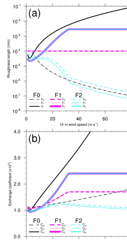
Figure 1.Plots of(a)roughness lengths and(b)bulk transfer co-efficients versus wind speed at 10 m height for neutral conditions. Flux schemes F0, F1, and F2 are colored black and gray, red and pink, and green. The thick solid curves arez0andCD, thin solid curves arezhandCH, and dashed curves arezqandCQ. It is noted that some curves are identical. For F1 and F2,z0(and thusCD) is the same; for F1 and F2 the respective heat and moisture roughness and coefficients are the same:zh=zqandCH=CQ.

Under neutral condition, the stability parameters(z+z0)/L and(z+zh)/Lare zero (see Eqs. A7, A8, and A9); therefore,

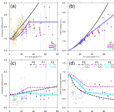
Figure 2.Plots of(a)momentum transfer coefficients,(b)friction velocity,(c)scalar transfer coefficients, and(d)transfer coefficient ratios versus wind speed at 10 m height from available observational estimates as found in the literature. The scalar transfer coefficients shown here can beCH,CQ, orCKupon the availability in the literature that we referred to in this study. The purple dots represent the values from Bell et al. (2012), blue circles represent values from French et al. (2007), dark green circles represent values from Geernaert et al. (1987), green curve represents values from Jarosz et al. (2007), red curve represents values from Large and Pond (1981), red dots represent values from Powell et al. (2003), blue dots represent values from Richter et al. (2016), and the orange dots represent values from Vickers et al. (2013). The curves are given by fitted equations; the circles represent the available data points; the dots represent average values in a range of wind speed bins with the bars showing the corresponding data spread as denoted by either the standard deviations or the 95 % confidence intervals, where the wind speed bin and the representation of data spread vary in the literature. Table B1 provides brief information of these observational estimates. The respective bulk parameters derived from WRF, represented as shown in Fig. 1, are superimposed for a comparison.

2.1.1 Momentum and moisture roughness length for flux option F0

For the default flux option (F0), the momentum roughness length is given as Charnock’s (1955) expression plus a vis-cous term, following Smith (1988):

z0=α u2_∗

g +

0.11v u∗

, (1)

3.0 m s−1(Fig. 1; black thick solid curve). A constant value ofα=0.0185 is used for F0.

The moisture roughness length is adapted from COARE 3.0 (Fairall et al., 2003) and expressed as a function of the roughness Reynolds number, with an additional lower limit of 2.0×10−9used in this option:

zq=max h

2.0×10−9,

min1.0×10−4,5.5×10−5R−_∗0.6i, (2) whereR∗=z0u∗/vis the roughness Reynolds number andv

the kinematic viscosity of dry air and a function of air tem-perature for theR∗calculation. The temperature roughness

lengthzhis set to equal tozq. The upper limit of 1.0×10−4

keeps the scalar roughness length invariant at extreme wind speeds (below approximately 4.0 m s−1), whereas the lower limit of 2.0×10−9is implemented to prevent the model from blowing up. Below this high wind speed, the heat and mois-ture transfer coefficients increase monotonically with wind speed (Fig. 1; gray thin solid and black dashed curves). For this option, the formulas of roughness lengths are different from that used by Green and Zhang (2013), where the vis-cous term forz0was given as a constant value of 1.59×10−5, zh is set equal toz0, andzq is set to a somewhat different

functional form ofz0andu∗.

2.1.2 Momentum and moisture roughness length for flux option F1

For the flux option 1 (F1), the momentum roughness length is expressed as a blend of two roughness length formulas (Green and Zhang, 2013):

z0=max1.27×10−7,

minzwz2+(1−zw) z1,2.85×10−3 i

, (3a)

zw=min

1, h u_∗

1.06 i0.3

, (3b)

z1=0.011 u2∗

g +1.59×10

−5_{, (3c)}

z2=

10 exp9.5u−∗1/3

+

0.11v max(u∗,0.01)

, (3d)

where the first roughness length formula (z1) is again the Charnock (1955) expression plus a constant value of the vis-cous term, with α=0.011, as suggested by Smith (1988). The second formula (z2) is the exponential expression from Davis et al. (2008) plus a viscous term; here a constant kinematic viscosityv=1.5×10−5m2s−1is used. The two roughness length formulas are combined using a weight function (zw), with a lower and upper limit onz0of 1.27× 10−7m and 2.85×10−3m, respectively. The lower and up-per limits on z0are adapted from Davis et al. (2008), with

a slightly different value of the lower limit. The upper limit used here acts to prevent a monotonic increase in the mo-mentum roughness length as well as the momo-mentum transfer coefficient, under high-wind conditions. The resulting curves present an increase with wind speed below 33.0 m s−1 but exhibit a leveling-off behavior starting at the wind speed of 33.0 m s−1(Fig. 1; red thick solid curves). The wind speed of 33 m s−1 is extremely close to the lower limit of maxi-mum wind speed for a typhoon. The use of thisz0formula re-sults in apparently smaller momentum roughness length and transfer coefficient at all wind speeds than that in F0. This leveling-off inCDwith wind speed suggests a decline in the

efficiency of the exchange of momentum across the air–sea interface (see Eq. A1). Considering that the drag effect acts as a momentum sink in the surface layer, it is expected that an atmospheric simulation using thez0 formula of F1 shall retain a larger portion of the total amount of near-surface mo-mentum at all wind speeds than that using the F0 formula, and such a difference in the transfer efficiency becomes in-creasingly significant with higher wind speeds because of the leveling-off behavior seen in F1.

F1 setszh=zq=10−4m for all wind speeds. Large and

Pond (1982) suggested constant values forzh andzq under

different conditions of stability, ranging from 10−9m (sta-ble) to 10−4m (unstable). The constant value of 10−4m used here corresponds roughly to the unstable condition in Large and Pond (1982). While using an invariant scalar roughness length, the heat and moisture transfer coefficients can still vary with wind speed (Fig. 1; pink thin solid and red dashed curves) because of the drag-dependent effect (see Eqs. A7, A8, and A9). Consequently, the heat and moisture transfer coefficients are also beginning to level off at the wind speed of 33.0 m s−1_.

2.1.3 Momentum and moisture roughness length for flux option F2

For the flux option 2 (F2), the momentum roughness length is the same as that for F1. The temperature and moisture rough-ness lengths are expressed based on the formula proposed by Brutsaert (1975a):

zh=z0exp h

−κ7.3R∗1/4Pr1/2−5 i

, (4)

zq=z0exp h

−κ7.3R∗1/4Sc1/2−5 i

, (5)

where R∗ is the roughness Reynolds number, κ is the von

Karman constant, Pr and Sc are the Prandtl and Schmidt

numbers, and 7.3 and 5 are experimental constants (Brut-saert, 1975b). As in F0, a temperature-dependentv is also used for R∗calculation. The values ofκ, Pr, and Sc are set

Reynolds number and Prandtl and Schmidt numbers. The re-sultingzh andzq are practically an exponential decay ofz0 with wind speed (Fig. 1; green thin solid and green dashed curves). The scalar roughness lengths in F0 and F2 both de-crease with wind speed, and their decreasing rates as well as magnitudes are similar at higher wind speeds. However, their resulting scalar transfer coefficients are apparently different. Unlike the monotonic increasing behavior found in F0, for F2 the heat and moisture transfer coefficients show an up-ward trend with wind speeds below 33.0 m s−1and then start decreasing at this wind speed. Such a discrepancy between F2 and F0 results from the drag-dependent effect in the scalar transfer coefficients (see Eqs. A7, A8, and A9).

2.2 Comparison between modeled and observational bulk transfer coefficients

Figure 2 presents the bulk transfer coefficients and friction velocity obtained from existing observational estimates as found in the literature. A brief description of these observa-tional estimates is provided in Appendix B. Overall, the be-havior ofCDin F1 and F2 as a function of wind speed is more

consistent with recent observations than that in F0 (Fig. 2a). Under the low- to moderate-wind conditions, all the flux op-tions generally predict similar behaviors to those observed in the observational estimates, and their values are within the observed data range. For the higher wind conditions, F1 and F2 predict a leveling-off inCDvalues with wind speed such

that it is significantly different from F0 starting at 33 m s−1. Considering the large discrepancy as well as the large spread of data found in the observational estimates beyond the wind speeds of approximately 55 m s−1_{, the leveling-off behavior} of CD values in F1 (and thus F2) is more reasonable than

the monotonic increasingCDvalues in F0 (Fig. 2a). This is

also supported by the comparison of the variations in friction velocity (Fig. 2b).

In Fig. 2 c, we plotted all observational estimates of scalar transfer coefficients (CH,CQ, andCK) available in the

liter-ature that we referred to for this study (Table B1). Visually, we see an upward trend between the data samples from Geer-naert et al. (1987) and French et al. (2007) but no significant trend between French et al. (2007) and the remaining two with higher-wind conditions (Bell et al., 2012; Richter et al., 2016). However, Geernaert et al. (1987) reported that their data were mostly collected under stable conditions. Studies have revealed a stability dependence ofCH, in which values

ofCHunder stable conditions are lower than those under

un-stable conditions (Large and Pond, 1982; Smith, 1988). Ac-cordingly, the applicability of the increases in CH andCQ

with wind speed remains elusive. Compared with F0, both F1 and F2 give a relatively reasonable pattern of CH and CQ, with F2 fitting the observational estimates better than

F1 does.

In the context of the leveling-off behavior ofCD at high

wind speeds as well as the absence of a monotonic increase

inCHandCQwith wind speed, both F1 and F2 provide more

reasonable formulas for parameterizing the surface fluxes than F0. Furthermore, F1 predicts largerCH andCQat all

wind speeds than F2 does, implying that F1 could gain larger enthalpy fluxes. Because the formula ofz0(and thusCD) is

identical in F1 and F2 while their respective formulas forzh

andzq are different, and because the behaviors of transfer

coefficients in F0 are quite distinct from those in F1 and F2, we use theCK/CD ratio to compare between the three flux

options. By assuming thatCH∼CQ∼CK here, we plot the

ratiosCH/CD andCQ/CD in Fig. 2d. All the flux options

present a decrease in the ratio with wind speed, except that for F1 an upward trend and leveling-off pattern are found under extremely low wind and high wind conditions, respec-tively. TheCK/CD derived from the available observational

estimates was also superimposed for reference. We noted that for moderate to high wind speeds, the values ofCK/CD are

all below the lower limit, namely 0.75, for mature hurricanes as suggested by Emanuel (1995). Even for F1, the ratio levels off at a value of 0.7. Relatively small value ofCK/CD,

com-pared with the lower limit of 0.75, is indeed not uncommon and has been reported by numerous studies based on observa-tional measurements (e.g., Drennan et al., 2007; Zhang et al., 2008; Bell et al. 2012) and numerical simulations (e.g., Hill and Lackmann, 2009; Green and Zhang, 2013). Nonetheless, we still can qualitatively relate the tropical cyclone inten-sity to the ratio ofCK/CD. Accordingly, F1 is expected to

have the highest potential to achieve the most intense storm among the three options because it has the highest values of CK/CD almost at all wind speeds. F0 has the lowest values

ofCK/CDowing to its largest values ofCD, thereby having

the lowest potential to produce a comparable storm intensity to F1.

2.3 Experimental designs

de-velopment of mesoscale processes near the surface. The Na-tional Centers for Environmental Prediction Global Forecast System (GFS; Environmental Modeling Center 2003, 2016) operational global analysis dataset was used to provide the initial and boundary conditions. The GFS global analysis has a horizontal resolution of 0.5◦, and it is also used as data for the grid nudging. The model sea surface temperatures (SSTs) were taken from the RTG-SST dataset (Gemmill et al., 2007), with daily time resolution; there was no ocean feedback in this study. The SSTs varied during the nudging stage up un-til 00:00 UTC on 5 November 2013 and thereafter remained fixed throughout the sensitivity simulation such that the dif-ferences in underlying SSTs between the flux options became negligible. Consequently, sensitivity of typhoon intensity and structure to the flux options (thus the surface flux formulas) can be determined to a large extent. All the sensitivity exper-iments started at 00:00 UTC on 5 November 2013 and ended at 06:00 UTC on 8 November 2013 (Fig. 3; red dots). All results are from within the 78 h that the experiments ran for.

Typhoon Haiyan formed in the western North Pacific on 3 November 2013 and underwent a rapid intensification a few days later. Haiyan reached peak intensity of 895 hPa before it made a cataclysmic landfall near Guiuan, Eastern Samar, Philippines, on 8 November 2013 at about 04:40 PHT (UTC+8). The storm then crossed the Philippines, migrated west-northwestward, and made its final landfall in Vietnam. Our simulation period for the sensitivity experiments covers the stages of Haiyan’s peak intensity and landfall. We focus on the mature stage of Haiyan before its landfall near Guiuan, Eastern Samar.

3 Temporal evolutions of track and intensity

All simulations show a similar west-northwestward move-ment toward land and appropriately follow the observed best track, but with slower translation speeds (Fig. 4a). The ty-phoon landfall at Samar island is delayed between 3 and 5 h in these sensitivity simulations. Because of the delayed landfall, we compare the evolution of the typhoon related to its longitudinal position (Fig. 4b). In general, the simu-lations continue to intensify and reach their peak right after 18:00 UTC on 7 November 2013 and before landfall. We re-fer to the time span from 18:00 UTC on 7 November 2013 to 00:00 UTC on 8 November 2013 as the mature stage of the simulated typhoon. In this study, the cumulus parameteriza-tion was used for all resoluparameteriza-tions. This is because we intend to keep consistency among all cases. Results from an additional simulation of the 1kmF0 with the cumulus parameterization turned off revealed that the simulated Haiyan intensity and structure are overall similar. The minimum central pressure and storm track of the 1kmF0 without cumulus parameter-ization follow almost the same evolution as that of 1kmF0 (Fig. S3). In our case, the use of a cumulus parameterization in high-resolution (1 km) simulation does not exert

consider-able influence on the typhoon intensity, track, and structure. Some studies have also revealed that the activation of cu-mulus parameterization for simulation with grid spacings of 2–3 km produced an overall similar simulated storm to the simulation with explicit convection (e.g., Yu et al. 2011; Li et al. 2018; On et al. 2018).

For each resolution group, F1 is the most intense in terms of minimum central pressure, whereas the intensity of F2 is somewhat between that of F0 and of F1. The intensity is sen-sitive to model resolution. Overall, the intensity increases as the resolution is changed from 6 to 3 km, but it significantly increases as grid spacing is reduced to 1 km. The experi-ment 3kmF1 yields an intensity level comparable with that of 1kmF0, demonstrating the benefit of using a more reasonable flux option in improving intensity simulation. Accordingly, the combination of the decrease in the momentum transfer coefficient (generally tends to reduce the energy loss) and increase in enthalpy transfer coefficients (thus more energy gain) has greater potential to yield a stronger storm. Finally, a higher resolution is more conducive to the intensification due to the change in flux formulas.

Figure 3.The model domain (red box) and calculation domains for the contoured frequency by altitude diagrams (blue box) and for energy spectra (cyan box). The red, tan, and green and dots represent the locations of Haiyan obtained from the best-track dataset. The red dots indicate the period of sensitivity experiments, the tan dots indicate the nudging period, and the green dots are the locations outside our simulation period.

Table 1.Summary of the resolutions and surface flux options tested. The nudging period for all experiments is between 00:00 UTC on 4 November 2013 and 00:00 UTC on 5 November 2013, with an identical nudging setting for each resolution group using the default flux option (F0). Thereby the corresponding sensitivity experiments start with an identical initial TC (tropical cyclone) structure and location. The MCP and MSW indicate, respectively, the minimum central pressure at the TC center and maximum surface wind speed near the TC center.

Experiment Resolution Flux Notes

name (km) option

6kmF0 6 0 Nudging stage: model resolution and flux option configured as 6kmF0

6kmF1 6 1 Initial TC: MCP=988.0 hPa and MSW=33.7 m s−1; 145.79◦E, 6.36◦N

6kmF2 6 2 Horizontal grid points: 538×367; time step: 20 s

3kmF0 3 0 Nudging stage: model resolution and flux option configured as 3kmF0

3kmF1 3 1 Initial TC: MCP=987.6 hPa and MSW=36.3 m s−1; 145.95◦E, 6.35◦N

3kmF2 3 2 Horizontal grid points: 1075×733; time step: 10 s

1kmF0 1 0 Nudging stage: model resolution and flux option configured as 1kmF0

1kmF1 1 1 Initial TC: MCP=986.5 hPa and MSW=36.9 m s−1; 145.88◦E, 6.46◦N

1kmF2 1 2 Horizontal grid points: 3223×2197; time step: 3 s

conditions, and geographical location, would be incorporated into these reference curves (Knaff and Zehr, 2007). The op-erational WPR may somewhat be considered the best fit to the actual mass–wind relation of TCs. The winds and pres-sures of Haiyan from the JTWC best-track data have been plotted in Fig. 4c, and the distribution agrees well with the JTWC operational WPR; we thereby omitted them from the plot. All our simulated wind pressure distributions present similar slopes to the two reference curves of 1 min averaged winds, indicating that these simulations are valid for further investigation of the typhoon structures.

Bao et al. (2012) reported that the simulated WPR is con-trolled by the formulation of the drag coefficient. From a

set of simulations for North Atlantic TCs between 2008 and 2011, Green and Zhang (2013) found that differentCD

ences in the wind pressure distribution between these sensi-tivity simulations are demonstrated by their magnitudes. For each resolution group, F1 is the most intense in terms of both minimum central pressures and maximum winds, whereas the intensity of F2 is somewhat between that of F0 and F1. A comparison of resolution groups used in F0 reveals a sig-nificant increase in intensity at higher resolutions during the mature stage (where the storm has a higher strength), with 1kmF0 receiving larger increments. The set of experiments using F1 presents a similar pattern, with the larger increments in 1kmF1 being much more marked.

In brief, increased resolution and more reasonable flux pa-rameterization (e.g., F1 in this case) can both improve ty-phoon intensity simulation to a certain extent. However, a sufficiently high resolution is more likely to the benefit from improved flux formulas. The implication is 2-fold. First, the use of reasonable flux formulas to improve intensity simula-tion is perhaps more efficient than using an extremely high resolution when computational resources are limited. Sec-ond, higher model resolution is conducive to improving sur-face flux representation in strong typhoon intensity simula-tions. The mechanisms underlying these two issues are no-table. We address the issue of higher model resolution and its effect on surface flux representation in the following sec-tions.

4 Storm structure at the mature stage

The sensitivity of simulated typhoon intensity to various res-olutions and flux options is also associated with changes in the simulated typhoon structure. To isolate differences be-tween simulations of different grid spacing, the hourly out-puts on the WRF native grid were transformed to the cylin-drical (polar-height) coordinate system centered at the simu-lated typhoon at each time point. To avoid spatial sampling issues in the comparison of mass and wind fields, all model outputs were transformed to an identical resolution setting. We used a 3 km horizontal resolution and an uneven vertical resolution with smaller spacing in the boundary layer for the cylindrical transformation. Specifically, the cylindrical coor-dinate used in this study has an azimuthal resolution of 2◦, a radial resolution of 3 km, and an uneven vertical resolu-tion within the radius and height of 900 and 18 km, respec-tively. All the data to be analyzed are interpolated from the model native coordinate to the cylindrical coordinate using bilinear interpolation. The zonal and meridional components of horizontal wind fields are transformed to tangential and radial wind components using their standard formulas. The (height-invariant) typhoon center is defined as minimum cen-tral pressure using the surface pressure field. We also exam-ined the geometric center for the local minimum pressure and found that the distances between the center at grid point and the geometric center are less that the half of the grid spac-ing, for the simulation period after 24 h (valid at 00:00 UTC

on 6 November 2013). The magnitudes of the vertical tilt of the center (in terms of the WRF output perturbation pressure field) are also small: about the size of one grid box. In this study, radial variations of model fields were all derived from these transformed subsets.

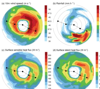
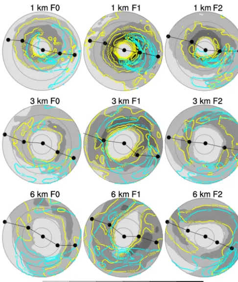
Figure 5 shows the horizontal distributions of wind speed at 10 m height, total rainfall, and surface enthalpy fluxes for F0 with 3 km resolution after the cylindrical transformation. The wind speed distribution shows a ring of higher wind speed (exceeding approximately 42 m s−1), with wider re-gions of high wind speed over the right side (northern semi-circle) of the track, with a partial ring of the maximum wind speed (∼50 m s−1), open to the west, at the range of radii 40–50 km. A region of intense rainfall is located on the left-rear side of the track. Regions of a larger amount of sur-face fluxes are located near the local maximum wind speeds; however, they are not necessarily co-located. This is because the near-surface enthalpy vertical gradient, other than wind speed, also influences flux calculation. The discrepancies in the horizontal distributions of surface fields between differ-ent resolution groups are more significant than those between flux options (Fig. 6). The 1 km resolution group yields a sig-nificant eyewall (in terms of these surface fields) contraction compared with the other two groups. The 3 km resolution group exhibits a relatively larger eye region, less contracted radius of the maximum wind speed, and total rainfall and surface fluxes. The 6 km resolution group does not present a well-defined eyewall structure in terms of these surface fields. Therefore, the increase in resolution from 6 to 3 km yields a better representation of the concentric pattern of the near-surface fields related to the typhoon center. In general, the use of different flux options results in the enhancement of these surface fields and, thus, the intensity in terms of the minimum central pressure and maximum wind speed, in the order F1>F2>F0.

cen-Figure 5.Horizontal distributions for(a)wind speed (m s−1) at 10 m height,(b) total rainfall (mm h−1),(c)surface sensible heat flux (W m−2), and(d)surface latent heat flux (W m−2) at forecast hour 71 h (valid at 22:00 UTC on 7 November) for the experiment F0 with 3 km resolution. All fields are taken from the transformed subset on cylindrical grids; see text for detail. At 71 h, the simulated typhoon centered at the nearest location to the best-track location at 18:00 UTC on 7 November 2013. Range rings are shown at radii of 20, 40, 60, 80, and 100 km. Black dot at the plane center denotes the simulated typhoon center at 71 h, whereas the two dots to the upper left and lower right of this central dot are the corresponding locations of the typhoon center in the next and previous 2 h. Solid lines connecting these dots denote the simulated typhoon track within the 5 h.

ter of Haiyan, almost the same as the direction of the vertical tilt. We also found similar vertical wind shear of approxi-mately 5 m s−1_{at a northeasterly direction, as well as a small} vertical tilt (about 1 grid box) of the storm center, during the 12 h period starting at 12:00 UTC on 7 November 2013 (data not shown). Accordingly, our simulations are in reasonable agreement with observations of Haiyan studied by Shimada et al. (2018).

The next step is to examine the azimuthal averages of the radius distribution for surface fields as well as the vertical structure of the simulated typhoon. For the radius distribu-tions shown in Figs. 7, 8, 10, and 11, the track lines over a 3 h window (the two segments centered at that particular hour, as shown in Fig. 5) were used to identify the semicir-cles on both sides. Because a small deflection of the track tendency is generally found in the 3 h window, the areas of the right (northern) and left (southern) semicircles are not necessarily the same.

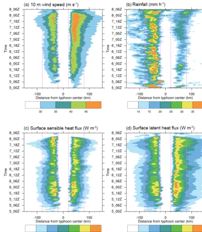
Figure 7 provides Hovmöller diagrams of the 10 m winds, total rainfall rate, and surface enthalpy (latent and sensible

Figure 6. Horizontal distributions for wind speed at 10 m height (shaded; m s−1), surface latent heat flux (yellow contours; W m−2), and total rainfall (cyan contours; mm h−1) at 71 h for all experi-ments. In all the experiments, the center location of the simulated typhoon at 71 h is at the nearest or the second nearest location to the best-track location at 18:00 UTC on 7 November 2013. The dis-tributions for experiment F0 of 3 km resolution are the same as in Fig. 5 but slightly zoom in on a circle of radius 80 km; range rings are shown at radii of 20, 40, 60, and 80 km. Other symbols are shown as in Fig. 5.

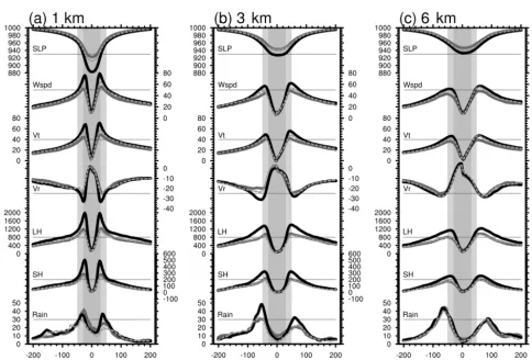
We begin with the composite of 3 km resolution (Fig. 8b). During the mature stage, the radial patterns of mean sea level pressure (SLP) and 10 m winds reveal the typical structure of a tropical cyclone. The difference between the radii of maxi-mum 10 m winds (RMWs) of 3kmF0 and 3kmF1 is insignif-icant. The tangential wind components dominate the 10 m wind fields. In both experiments, the radii of the maximum radial wind component are slightly larger than those of their respective tangential winds. In the context of azimuthal aver-ages, the radial distributions of surface enthalpy fluxes are fundamentally constrained by the 10 m wind speed inten-sity. The aforementioned asymmetric pattern is again evident in the rainfall distribution and even in the wind fields. The 3kmF1 experiment yields a deeper storm central pressure and stronger wind speeds and enthalpy fluxes than the 3kmF0 ex-periment does. The 3kmF2 exex-periment produces similar pat-terns to the 3kmF0 experiment. The majority of these incre-ments occur around the eyewall (in terms of the maximum

winds). Increasing the grid spacing to 6 km yields a com-posite radial structure highly similar to the 3 km group, thus indicating the relationship among these near-surface fields (Fig. 8c). The major difference between the groups (6 and 3 km) is the size of the inner core with respect to the eyewall radius (measured in RMWs) and the sharpness of peaks in the near-surface fields. This is consistent with the aforemen-tioned horizontal distributions of these surface fields shown in Fig. 6. As grid spacing decreases, RMWs decrease and the peak sharpness in winds and enthalpy fluxes increase. A much more marked decrease in RMWs and increase in peak sharpness are found in the 1 km resolution group than in the other groups (Fig. 8a). The SLPs, wind fields, and enthalpy fluxes in the 1 km group have narrow but sharp peaks, along with larger peak values compared with the other resolution groups. The asymmetric pattern of the wind fields is less ev-ident but still can be seen. The 1kmF1 experiment yields a much stronger storm than the 1kmF0 experiment. The asym-metry of the rainfall pattern, however, decreases by using F1. At this point, whether the reduction of grid spacing or the use of more realistic flux formulas leads to a more symmet-ric (and thus more intense) tropical cyclone remains unclear. In brief, both the increased resolution and more reason-able flux formulas enhance storm strength. Storm size (in terms of RMWs) is apparently sensitive to the changes in grid spacing but less sensitive to the choice of flux options. A reduction of storm size with smaller grid spacing has been noted by numerous studies (e.g., Davis et al., 2008; Fierro et al., 2009; Gentry and Lackmann, 2010; Kanada and Wada, 2016). As the strength of a storm increases, the eyewall con-tracts, indicating a higher efficiency of storm intensification with smaller grid spacing. In our work, the effect of differ-ent flux formulas on Typhoon Haiyan simulation is revealed by the changes in storm central pressure and the intensity of maximum winds and enthalpy fluxes around the eyewall. This implies that the underlying mechanisms (i.e., surface flux exchange processes) of various flux options account for storm intensity, whereas the reduction of grid spacing leads to more intense storm structures providing more conducive conditions for enhancing a positive flux effect.

Figure 7.Radius–time cross sections of(a)10 m wind speed (m s−1),(b)rainfall (mm h−1),(c)surface sensible heat flux (W m−2), and(d) surface latent heat flux (W m−2) for the control experiment (3kmF0). The positive and negative distances from the typhoon center represent the azimuthal averages of the right (northern) and left (southern) semicircles, respectively, along the typhoon track. For each hourly output, the corresponding track in 3 h centered at that particular hour is used to identify the semicircles on both sides.

F1. This can also explain the comparable maximum wind speeds found in the F1 experiments with 3 and 6 km resolu-tion (see Fig. 4c). The comparable storm intensities, in terms of minimum central pressure, found in 3 and 6 km resolutions (see Fig. 4b) are indeed in association with different near-surface wind speed distribution (also see Fig. 6). In 3 km as well as 1 km resolution, more extended and organized areas of extremely high wind speeds are found, whereas for 6 km resolution, broader areas of high wind speeds with a small amount of extremely high wind speed patches are found.

The previous analyses indicate that the typhoon intensity is mainly controlled by the model resolution. The near-surface wind speed is an influential factor for the calculation of bulk transfer coefficients. Considering the low frequency of occur-rences for extremely high wind speeds, the positive effect of the more reasonable surface option (F1) cannot be enhanced efficiently with a relatively large grid spacing of 6 km.

in-Figure 8.The radial variations of surface fields for experiments 1 km(a), 3 km(b), and 6 km(c). The surface fields shown are (from top to bottom) sea level pressure (SLP; hPa), wind speed and tangential and radial winds at 10 m (Wspd, Vt, and Vr; m s−1), surface latent and sensible heat fluxes (LH and SH; W m−2), and total rainfall (Rain; mm h−1). Positive values of Vr indicate inflow. Gray, black, and gray-dashed curves represent flux options F0, F1, and F2, respectively. Horizontal gray lines are selected reference lines for each field. All fields are time averaged between 18:00 UTC on 7 November 2013 and 00:00 UTC on 8 November 2013. Positive and negative distances represent the right (northern) and left (southern) semicircles as in Fig. 7. Vertical light-gray and gray shaded bars denote the radial sectors bounded by radii of 50 and 30 km, respectively.

creases to up to 3 km or higher. This is consistent with the findings of Davis et al. (2008) and Gentry and Lack-mann (2010) that a resolution of approximately 3 km or higher is required for significant improvement of intensity simulation of intense hurricanes (Hurricane Katrina in their case). With a lower resolution, 6 km in our case, we spec-ulate that the momentum energy is diluted over the nearby grid points such that limited magnitude (higher but not ex-treme) of wind speeds would become evenly distributed over a broader area. This idea is specifically inspired by the stud-ies of Bryan et al. (2003) and Miyamoto et al. (2013). We further discuss the energy distribution of these simulations in the next section.

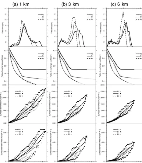
The behaviors of CK/CD show that the patterns almost

strictly follow their respective curves as predicted by the cal-culation of the neutral condition using the pseudo-wind data (see Fig. 2d). The spread of data, as represented by the range, is rather small and is approximately 10 %–12 % of the mag-nitude of their respective binned averages. However, the

F1 can achieve. Although the extremely high wind speeds comprise a small percentage of the eyewall circulation of a mature cyclone, they have a crucial role in enhancing surface fluxes that supply enthalpy to the eyewall.

As the resolution increases, the vertical distribution of tan-gential winds reveals a significant increase in the vertical ex-tent of stronger wind speed, a reduction of the outward slope of the maximum wind axis, and thus a contraction of the eye-wall (Fig. 10). With the change from F0 to F1, tangential wind speeds increase, with an outward and upward expansion of the region of stronger wind speed. No apparent changes are noted in the vertical slope and radius of the eyewall ow-ing to the change in flux options. Both the composite inflow and outflow weaken as the resolution increases but enhance as the flux option changes from F0 to F1. Here, the maximum value of inflow (outflow) is 28.3 (−38.8) m s−1in 1kmF0 but it is 33.6 (−44.5) m s−1_{in 1kmF1. Moreover, the maximum} cores of tangential winds descend and the depth of inflow decreases as the resolution increases. Overall, the patterns of F2 are somewhat between those of F0 and F1. In addition, we can see that the upper-level radial inflows are evident in the 1 km resolution group. The upper-level radial inflows are ap-parently weaker in the 3 km resolution group and are hardly found in the 6 km resolution group. The upper-level radial inflow above the upper outflow layer is related to the devel-opment of upper-level warming in the eye; this is addressed in Fig. 12.

The contraction of the eyewall with reduction of grid spacing is also revealed by a more upright eyewall updraft (Fig. 11). We start with the major eyewall updrafts and down-drafts as denoted by red and blue contours, respectively, in Fig. 11. The reduction of grid spacing also results in stronger updrafts and downdrafts, where the enhanced eyewall down-drafts may be a cause of the decrease in the depth of inflow. The convections outside of the eyewall (weaker upward ve-locity denoted by the pink hatched area) are apparent in the 1 km resolution group. For this resolution group, the outside convection in F1 is stronger than that in F0. The outside con-vection is a result of the azimuthally averaged upward veloc-ity of the outer rainband. In the 3 km resolution group, the outside convections are weaker but still apparently shown. No outside convection can be clearly distinguished from the eyewall in the 6 km resolution group. As the resolution de-creases, the model may not be able to resolve intense updraft cores in the eyewall as well as the outer rainband near the eyewall. The larger grid spacing can only resolve a broader area of weaker updraft instead. We further discuss this in the next section. Stronger inflow and outflow as well as broader eyewall updraft are found at the 6 km resolution, suggesting that secondary circulation is stronger at lower resolutions, similar to the finding of Fierro et al. (2009). We further ex-amined the horizontal flow patterns near the altitudes of the upper outflow layer, both on model native grids and cylindri-cal grids, and confirmed that the upper-level flow patterns in the 6 km resolution group are more radially outward than the

rotational component. As the resolution increases, the upper-level flow pattern becomes more rotational, and the radially outward component is suppressed. Because of such discrep-ancy in the upper-level flow pattern, the azimuthally averaged upper outflows (upper-level radial winds) in the 6 km resolu-tion group are the strongest between the resoluresolu-tion groups.

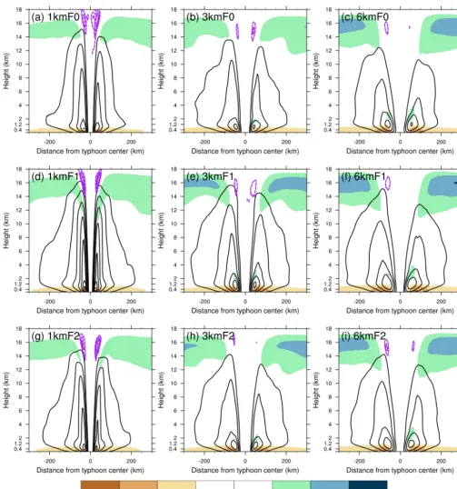
The time evolution of the core temperature is represented by the temperature anomaly with respect to a reference mean temperature (Fig. 12). Here we term the positive temperature anomaly as warming. The distinct difference found among the resolution groups is the development of the upper-level warming layer within the eye. For the 1 km resolution group, the apparent upper-level warming layer appears above ap-proximately 10 km within a deep warming column in the eye. The upper-level warming layers occur earlier in the experi-ments F1 and F2 (Fig. 12a, d, g). The warming layer in ex-periment 1kmF1 is the most intense among all the others. The timings of the upper-layer warming are associated with their respective upper-level radial inflows. The upper-level warm-ing layer has long been recognized by observational studies (e.g., Hawkins and Imbembo, 1976) and numerical simula-tions (e.g., Zhang and Chen, 2012; Chen and Zhang, 2013; Wang and Wang, 2014). In recent years, the formation of the upper-level warming layer has been related to the rapid inten-sification of tropical cyclones (e.g., Zhang and Chen, 2012; Chen and Zhang, 2013; Wang and Wang, 2014). This upper-level warming layer, under hydrostatic balance and consid-ering the enhanced effect due to the upper-level dryer and thinner conditions of air, can produce a much greater effect on the surface pressure falls than the lower-level warming (e.g., Zhang and Chen, 2012). Regarding the formation as well as the maintenance of the upper-level warming layer, Zhang and Chen (2012) emphasized the contribution from the high-potential-temperature air detrained from the lower stratosphere, whereas Chen and Zhang (2013) introduced the contribution from the air detrained from the convective bursts (anomalous intense updrafts) in the eyewall. Both studies revealed the importance of the upper-level radial inflow in the warm air detrainment onto the eye region. Wang and Wang (2014) reported that, in an environment with decreas-ing vertical wind shear, air detrained from the lower strato-sphere as well as from the convective bursts could result from the development of convective bursts within the inner-core region.

Figure 11.The same as Fig. 10 but for vertical velocity (contours; m s−1) and radial wind (color shaded; m s−1). Positive (upward) and negative (downward) velocities are indicated by red and blue contours, respectively, and are plotted every 1 m s−1starting from wind speeds of 0.5 m s−1. In addition, pink hatched areas denote an upward velocity of 0.3–0.5 m s−1; cyan contours denote a downward velocity of

of the upper-level warming layer can also be found in the 3 km resolution group, but apparently weaker than that in the 1 km group. However, the development of upper-level ra-dial inflow appears to precede the main warming for nearly 24–36 h. This may be partly attributed to the weaker con-traction of the eyewall in the 3 km resolution group. The weaker upper-level radial inflow is perhaps another reason for this inconsistency in the time evolution. The 6 km resolu-tion group does not present comparable development of this upper-level warming layer as in the 3 km group, again indi-cating that a resolution of 6 km is inadequate to resolve the details of structure and development of a strong typhoon like Haiyan (2013).

When the resolution increases, a more intense convection core can be resolved, leading to a rapid pressure decrease near the typhoon and a pressure gradient increase in the area. This change in the pressure field is presumably due to the en-hanced diabatic heating near the typhoon eyewall. The larger pressure gradient force would reduce the RMW according to the gradient wind balance equation. The reduced RMW would then accompany an area of diabatic heating closer to the typhoon center. This contraction of the eyewall keeps de-creasing the central pressure of the typhoon, yielding pos-itive feedback for typhoon development. The enhancement of these processes is mainly related to the model grid spac-ings. Near-surface wind speed affects the calculation of bulk transfer coefficients. The positive effect of the more reason-able surface option (F1) cannot be enhanced efficiently un-less an extremely large wind speed is generated through the reduction of grid spacing.

5 Statistical and energy spectral analyses

Several studies have reported that the reduction of grid spac-ing yielded a deeper, stronger, and more upright and con-tracted eyewall (e.g., Fierro et al., 2009; Gentry and Lack-mann, 2010; Kanada and Wada, 2016). We also demonstrated that the size of updraft cores in the eyewall shrank and the region of downdraft increases as the resolution is increased. Furthermore, both updraft and downdraft become more in-tense with the reduction of grid spacing. These features have also been recognized in many studies (e.g., Fierro et al., 2009; Gentry and Lackmann, 2010; Gopalakrishnan et al., 2011; Kanada et al., 2012). In addition, large vertical trans-port of heat and moisture can result in stronger storms given that the model resolution is sufficiently high (e.g., Gopalakr-ishnan et al., 2011; Kanada et al., 2012).

We used contoured frequency by altitude diagrams (CFADs; Yuter and Houze, 1995) to examine the variabil-ity of convective cores over the region shown in Fig. 3 (the blue box). The CFADs is a statistical method for summa-rizing the vertical distributions of meteorological fields. A CFAD is constructed by collecting frequency distributions of a particular variable at evenly spaced altitudes within an

area, compiling them into a two-dimensional (data bin and altitude) dataset, and portraying the data on a single contour plot. The ordinate in the plot represents the altitude variation, and the abscissa represents the frequency bin. For each alti-tude on a CFAD, the frequencies should add up to 100 %. For a given CFAD, each point depicts the frequency of oc-currence of the data in that bin at a specific altitude. Ac-cordingly, the CFADs ignore horizontal variability and pro-vide a bulk statistical measure for comparing the vertical structure of evolving fields of cumulonimbus clouds or any convective systems. Here, we take Fig. 13a as an example. On this CFAD, there are higher percentages (e.g., bounded by 20 % of data per decibel relative toZ per kilometer, or % dBZ−1km−1) found in the higher reflectivity bins at lower altitudes and found in the lower reflectivity bins at higher al-titudes. The former can indicate convective cells or precip-itations, whereas the latter can indicate snow or stratiform precipitation. Therefore, considering a set of CFADs for an evolving cumulonimbus clouds, say from the initiation to the mature stage, the maximum percentage at each altitude would change from vertically oriented to negatively tilted to-ward lower reflectivity values. More detailed interpretations of the use of CFADs can be found in the work by Yuter and Houze (1995).

interpreta-Figure 13.The CFADs of simulated reflectivity for experiments(a)1kmF0,(b)3kmF0,(c)6kmF0,(d)1kmF1,(e)3kmF1,(f)6kmF1,(g) 1kmF2,(h)3kmF2, and(i)6kmF2. The sampling time for model output is taken as the simulated typhoon centered at its nearest location to the best-track location at 18:00 UTC on 7 November 2013 and for the following 2 h. The simulated reflectivity was taken from all grid points with updraft (positive vertical velocity) within the calculation domain for CFADs (see blue box in Fig. 3 for the corresponding area) in the model native grids. For reflectivity CFADs, the bin size is 5 dBZ and the plot is contoured at 0.01 %, 0.1 %, 1 %, 5 %, 10 %, 20 %, 30 %, 40 %, 50 %, and 60 % of data per decibel relative toZper kilometer (% dBZ−1km−1), with the 20 % dBZ−1km−1contour highlighted in black and the lowest two contours displayed in magenta.

tions are different for reflectivity associated with updraft and downdraft here.

We further conducted CFADs of vertical motions to ad-dress this issue (Fig. 15). Most vertical velocities, carried by approximately 95 % of the data points as indicated by the re-gion within the 1 % of data per meter per second per kilome-ter (% m−1s km−1) contour, are apparently less than 5 m s−1 in all simulations. A similar pattern of CFADs of vertical ve-locity, revealing that most common values of vertical veloc-ity are substantially low, can be found in numerical simu-lations for TCs (Fierro et al., 2009; Gentry and Lackmann, 2010; Wang and Wang 2014) and observational data for cu-mulonimbi (Yuter and Houze, 1995). Furthermore, the region of upward motion is larger than that of downward motion in general. A similar asymmetry of the distributions of upward and downward motion was evident in simulations in previ-ous studies (Fierro et al., 2009; Gentry and Lackmann, 2010; Wang and Wang, 2014). In Fig. 15, the most significant

dif-ferences in the CFADs of vertical velocity are revealed by the lower frequencies, namely the values of 1 % m−1s km−1 and 0.1 % m−1s km−1. As the resolution increases here, both upward and downward motion present an expansion of the distribution of the frequency of 1 % m−1s km−1. However, the extents of the changes in upward and downward motions with resolution are different. In all simulations, the changes in the downward motion with an increased resolution are more significant than those in the upward motion. Therefore, the region (occurrence) of the downward motion increases as the resolution increases. The results also indicate the pres-ence of less downdrafts in lower-resolution simulations (i.e., 3 and 6 km), and the degradation of available data points can result in large biases in the CFADs of reflectivity in associa-tion with the downdraft.

Figure 14.The same as Fig. 13 but for CFADs of simulated reflectivity with downdraft.

contour) in 1 km simulations may be associated with much more intense updrafts compared with those in the 6 km sim-ulations. This is consistent with the discrepancy between the secondary circulations of different resolutions in the previous section, where 6 km simulations presented relatively wider and weaker updrafts among the different resolutions. As pre-viously mentioned, the CFADs of reflectivity in the 6 km simulations presented a relatively concentrated range of re-flectivity magnitudes compared with the 1 km simulations, implying that the convective cells associated with the eye-walls may be broader in spatial scale. This is confirmed by an examination of horizontal distributions of the reflectivity of the 6 km resolution of simulations (data not shown). This can be interpreted as follows. As the resolution is insufficient to resolve the typical cumulonimbus size (∼10 km), a num-ber of convective cells (e.g., cumulonimbus clouds) would be interpreted as a broader and perhaps stronger convective plume as discussed by Bryan et al. (2003) and Miyamoto et al. (2013). Bryan et al. (2003) attributed this broader convec-tive plume to the diffusion due to subgrid-scale processes. In short, the intense reflectivity (convective) cores of the 1 km simulations are driven by extreme updrafts occurring within a rather small fraction of the CFAD’s computational domain,

whereas the 6 km simulations are driven by relatively weaker updrafts spread over a much broader spatial distribution.

Figure 15.The same as Fig. 14 but for CFADs of simulated vertical velocity. The velocity bin size is 1 m s−1and the plot is contoured at 0.01 %, 0.1 %, 1 %, 5 %, 10 %, 20 %, 30 %, 40 %, 50 %, and 60 % of data per meter per second per kilometer (% m−1s km−1), with the 20 % m−1s km−1contour highlighted in black and the lowest two contours displayed in magenta.

options are similar, only the experiments with F0 and F1 were plotted in Fig. 16. In all simulations, for the KE spec-tra derived from the horizontal velocity components, we find a model effective resolution of approximately 7 DX where the values of the KE spectra drop significantly, as indicated by Skamarock (2004). Although the vertical velocity spec-tra exhibit a flatter slope than the horizontal KE specspec-tra, they also present apparent energy drops at wavelengths of approx-imately 6–7 DX. Our vertical velocity spectra show a pat-tern (i.e., the slopes) that is somewhat different from that of Bryan et al. (2003) with respect to the absence of peak values around the respective model effective resolutions. Bryan et al. (2003) conducted simulations with horizontal resolutions much higher than 1 km: 500, 250, and 125 m. With their ex-tremely high resolutions, more intense convections could be resolved. They indicated that a model resolution of 1 km re-mains insufficient for explicitly resolving convective clouds. Here, we speculate that insufficient intense convection cores in our simulations may result in the absence of peak values around the respective model effective resolutions.

Finally, the slope of the physical portion of the spectra (for the horizontal and vertical components, respectively)

re-mains essentially unchanged as the model resolution is var-ied. In general, the higher the resolution, the further the downscale extent is, the smaller the scales represented are, and the smaller the model effective resolutions reached are. The aforementioned descriptions remain true for all flux op-tions and averaging layers in our work. The key point is that the effective resolution is determined by grid spacing, not the flux options. We noted some subtle differences between the F0 and F1 experiments at smaller wavelengths at nearly 2 DX in the KE spectra but in only a few hours of the entire simulation period. In short, although the use of more reason-able flux formulas can increase simulated storm intensity to some extent, the positive effect of the flux formulas cannot be efficiently enhanced unless the grid spacing is appropriately reduced to yield intense and contracted eyewall structure.

6 Conclusions

Figure 16.Mean KE spectra for horizontal wind(a, b)and vertical velocity(c, d)for all simulations as computed over the boundary layer (a,c; between 1 and 2 km) and free troposphere (b,d; between about 3 and 8 km) for the mature stage. The mature stage is indicated by the average between 18:00 UTC on 7 November 2013 and 00:00 UTC on 8 November 2013. The gray lines correspond to the expected slopes for the large scale (−3 slope) and mesoscale to smaller scales (−5/3 slope) of the atmospheric kinetic energy spectrum. The wavelength and wavenumber are given on the lower and upperxaxes, respectively. The purple triangles in each panel, from left to right, denote the locations of 7 DX for the simulations of resolutions 6, 3, and 1 km, respectively. The domain of the spectral decomposition is shown in Fig. 3.

air–sea flux parameterization through the inner-core structure and spectral analyses. Specifically, we found significantly increased sensitivity of TC intensity simulations to surface flux parameterizations when model resolution approached the convective scale (∼1 km).

Three sets of surface flux formulas in the WRF model were tested using grid spacings of 1, 3, and 6 km. Increased reso-lution and more reasonable flux parameterization could both improve typhoon intensity simulation to a certain extent, but their effects on storm structures differed. A combination of decreasing momentum transfer coefficient and increasing en-thalpy transfer coefficients tends to yield a stronger storm. The storm size (in terms of the radius of maximum winds) is apparently sensitive to the changes in grid spacing. The choice of flux formulas had little effect on storm size.

Suf-ficiently high resolution was more conducive to the positive effect of flux formulas on simulated typhoon intensity.

The analysis of the CFADs revealed that the size of up-draft cores in the eyewall shrinks and the region of downup-draft increases, and both updraft and downdraft become more in-tense as the resolution increases. Therefore, the inin-tense re-flectivity (convective) cores of the higher-resolution simu-lations are driven by more intense updrafts within a rather small fraction of the spatial area, whereas lower-resolution simulations are driven by relatively weaker updrafts spread over a much broader spatial distribution. This resolution de-pendence of the spatial scale of updrafts is attributable to the model effective resolution based on the analysis of KE spec-tra. The effective resolution is determined by grid spacing, not the flux options. The analyses indicate that typhoon in-tensity is mainly controlled by the model resolution. Higher frequency of occurrences for extremely high wind speeds can be found in experiments with higher resolution. The near-surface wind speed is an influential factor for the calculation of bulk transfer coefficients. Although the use of more rea-sonable flux formulas can increase the simulated storm in-tensity to some extent, the positive effect of surface flux for-mulas cannot be efficiently enhanced unless the grid spacing is properly reduced to yield intense and contracted eyewall structure.

Although both updraft and downdraft cores within the eye-wall can be partially resolved at 1 km grid spacing, model convergence does not emerge here (e.g., Bryan et al., 2003; Gentry and Lackmann, 2010; Miyamoto et al., 2013). The conducive effect for grid spacing well below 1 km to the contribution of flux parameterization needs to be further explored. Finally, the typhoon intensity in the experiment 1kmF1 is apparently overestimated. Green and Zhang (2013) suggested that the overestimation of their simulated TC in-tensity, compared with the observed best track, may be par-tially attributed to the neglect of ocean feedback in the model. This is also true in our case. Other components of the numeri-cal model such as boundary layer mixing and the inclusion of wind wave coupling as well as ocean coupling are related to air–sea flux estimates, which is important for ocean feedback (e.g., Davis et al., 2008; Chen et al., 2007, 2010; Zhao et al., 2017). This is beyond the scope of this paper; however, fur-ther relevant research and additional simulation comparisons to other storms for generalizing our results are warranted.

Data availability. The National Centers for

Environmen-tal Prediction Global Forecast System (GFS) operational

global analysis dataset can be downloaded from the

web-site https://www.ncdc.noaa.gov/data-access/model-data/

model-datasets/global-forcast-system-gfs/ (last access:

20 July 2019; Environmental Modeling Center 2003,

2016). The RTG-SST dataset is available for download

at ftp://polar.ncep.noaa.gov/pub/history/sst/ (last access: 20 July 2019; Gemmill et al., 2007). The WMO subset of the IBTrACS (IBTrACS-WMO, v03r09) can be accessed at ftp://eclipse.ncdc.noaa.gov/pub/ibtracs/v03r09/wmo/ (last access:

Appendix A

(a) Fluxes in the atmospheric surface layer

In the surface layer, the vertical fluxes of horizontal momen-tumτ, sensible heat H, and latent heat LH near the surface are generally parameterized using bulk flux formulations: τ =ρu2_∗=ρCD(Ua−Us)2=ρCD(U )2, (A1)

H= −ρcpu∗θ∗= −ρcPCHU (θa−θs) , (A2)

LH= −ρLvu∗q∗= −ρLvCQU (qa−qs) , (A3)

whereρis the air density;cpthe specific heat capacity of air at constant pressure; Lv the latent heat of vaporization;u∗

the friction velocity, a velocity scale for the turbulent flow;θ∗

andq∗the scaling parameters for potential temperatureθand

specific humidity q, respectively; andCD,CH, andCD the

dimensionless bulk transfer coefficients for momentum, sen-sible, and latent heat, respectively. The vertical differences in horizontal velocity, temperature, and specific humidity are enclosed in the parentheses in their respective bulk formu-las, where the subscripts a and s denote the variable at a reference height and on the ground or water surface, respec-tively. Moreover, 10 m is frequently assumed as the reference height. The three bulk transfer coefficients should all corre-spond to the same reference height above the surface. Be-cause the wind speed just on the ground surface is zero and the surface current over water may be set to zero for the sake of simplicity, the bulk formula for the vertical flux of the hor-izontal momentum can be reduced toρCD(Ua)2; thereafter,

we omit the subscriptafor brevity. (b) Surface layer scheme in WRF

In WRF, the scaling parameters, bulk transfer coefficients, and all surface fluxes (momentum, sensible heat, and latent heat) are parameterized in a surface layer scheme. There are eight surface layer schemes available in the WRF-ARW, and seven of them are constructed based on the Monin–Obukhov similarity theory with somewhat different formulations, in-cluding those of the roughness lengths, bulk transfer coeffi-cients, and the nondimensional stability functions defined for wind and potential temperature profiles. Among these avail-able schemes, the surface layer scheme based on MM5 pa-rameterization (Grell et al., 1994) has been widely used for a broad range of atmospheric research. In this study, we used the revised version of the MM5 surface layer scheme that has been implemented in the WRF model before version 3.2 (Jiménez et al., 2012). Considering that some details of the scheme can change over time, we compared the correspond-ing routines in WRF-ARW to the formulations in Jiménez et al. (2012) and found some discrepancies. During the time of writing this article, we referred to the WRF routines wher-ever there is a discrepancy found. Below, we briefly describe the most relevant features of the revised MM5 scheme for our work. Because our focus is on the TC intensity over the

ocean, we only document the bulk transfer coefficients over the water surface.

(c) Flux parameterization used in this study

Based on the Monin–Obukhov flux–profile relationship, the scaling parametersu∗andθ∗are given as follows:

u∗=

κU

lnz+z0 z0

−ψm z+z_L0+ψm z_L0

, (A4)

θ∗=

κ (θa−θs)

lnz+z0 z0

−ψh z+z_Lh+ψh z_Lh

, (A5)

where κ is the von Karman constant; L is the Obukhov length;z is a specific height level; and z0 andzh are the

roughness lengths for momentum and sensible heat, respec-tively. All roughness lengths are in meters. The Obukhov lengthLcan be calculated from the relation

L= u 2

∗θa κgθ∗

, (A6)

where g is the gravitational acceleration. The Monin– Obukhov stability functions for momentum (ψm) and heat (ψh) are calculated according to variant stability regimes de-fined in terms of the bulk Richardson number. The details of the stability functions can be found in Jiménez et al. (2012). The scaling parameter, as well as the stability function for moisture, is assumed to be the same as that for the sensible heat.

The bulk transfer coefficients for momentum and sensible heat are given as follows:

CD=

κ2 h ln z+z0 z0

−ψm z+z_L0+ψm z_L0

i2, (A7)

CH=

κ2 h

lnz+z0

z0

−ψm z+Lz0

₊

ψm zL0 i h

lnz+zh

zh

−ψh z+Lzh

₊

ψh zLh i

, (A8) The bulk transfer coefficient for latent heat over water surface is given as follows:

CQ=

κ2 h

ln

z+z0

z0

−ψm z+Lz0

+ψm zL0

i h ln

_z+z

q

zq

−ψh

_z+z

q

L

+ψh zq

L

i, (A9)

wherezq is the roughness length for latent heat. Jiménez et

al. (2012) expressed the stability parameter as(z+z0)/Lin their formulas of CH and CQ (see their Eqs. 21 and 22).

In this version of the revised MM5 scheme,(z+zh)/Land (z+zq)/Lare used forCH andCQ, respectively.

Further-more, the first term enclosed in the second bracket on the right side of the CQ formula is mainly valid for land

sur-face as presented in Jiménez et al. (2012; see their Eq. 22). In our Eq. (A9), the corresponding term is expressed as ln z+zq/zq

According to the formulations of CD, CH, and CQ, the

behaviors of these bulk transfer coefficients are strongly de-pendent on the momentum and scalar (heat and moisture) roughness lengths (see Eqs. A7, A8, and A9). The contri-bution of momentum roughness length z0 is perhaps more significant than the rest of two. On the right side of theCD

formula, the three terms inside the bracket in the denomina-tor are expressed in terms of z0. Here, we term the whole expression with brackets in the denominator in Eq. (A7) as a drag-dependent effect. A comparison of these formulas indi-cates that the expressions inside the first brackets on the right side of the CH andCQ formulas are both identical to the

expression of the drag-dependent effect in Eq. (A7). In this context,CH andCQshall vary with wind speed due to the

drag-dependent effect even with an invariant scalar rough-ness length.

Appendix B

Table B1 provides brief information of the observational esti-mates shown in Fig. 2. For low-wind-speed conditions (wind speed roughly less than 5 m s−1), Vickers et al. (2013) in-dicated a decrease in CD with wind speed, in agreement

with that observed in COARE 3.0 (Fairall et al., 2003; their Fig. 5), whereas Geernaert et al. (1987) and Large and Pond (1981) suggested a nearly constant (no trend) CD. For moderate-wind conditions (approximate range of 5–

20 m s−1), Large and Pond (1981) and Vickers et al. (2013) indicated that the momentum transfer coefficientCD

mono-tonically increases with wind speed (see Fig. 2a). An upward trend ofCDhas also been reported in Geernaert et al. (1987)

and French et al. (2007), although the spread of their re-spective data is large. This is because shown in Fig. 2 are their data points rather than binned averages or fitted curves. Three sets of available estimates (Jarosz et al., 2007; Pow-ell et al., 2003; Richter et al., 2016) revealed that the up-ward trend in CD would cease under high-wind conditions

(approximate range of 25–55 m s−1), where a leveling-off or even a downward trend would occur instead. According to these observational estimates, the turning points of the wind-speed-dependentCDvariations were varied and found within

a range of 30 to 40 m s−1. Under the much stronger wind conditions (exceeding 55 m s−1), the behavior of CD again

differs considerably from the relatively lower range of wind speeds. Bell et al. (2012) and Richter et al. (2016) suggested a rebound ofCDvalues with wind speeds up to approximately

70 m s−1_{. However, there are also larger spreads of theC}

D

values found.

There are fewer observational estimates of the heat and moisture transfer coefficient reported in literature, com-pared with the momentum transfer coefficient. Practically, the transfer coefficient for moist-air enthalpy surface flux (CK) was estimated in a number of studies (e.g., Zhang et al.,

2008; Bell et al., 2012; Richter et al., 2016). A similar

expres-sion to Eqs. (A2) and (A3) can be derived for the moist-air-specific enthalpy flux, where the moist-air-specific enthalpy is given ase=cpT+Lvq (Emanuel, 1995). Most studies suggested that the bulk transfer coefficients for scalar fields (i.e., sen-sible heat and moisture as well as enthalpy) are nearly in-dependent of wind speed, with their respective mean val-ues being 0.7 to 1.5×10−3 (e.g., Geernaert, 1987; Smith, 1988; Drennan et al., 2007; Zhang et al., 2008; Bell et al., 2012; Richter et al., 2016). However, Fairall et al. (2003) re-ported a steady increase inCQwith wind speed based on the