Measuring Strategic Communications

(1)

University of South Carolina

Scholar Commons

Theses and Dissertations

2016

Modern Estimation Problems in Group Testing

Md Shamim Sarker

University of South Carolina

Follow this and additional works at:https://scholarcommons.sc.edu/etd

Part of theStatistics and Probability Commons

This Open Access Dissertation is brought to you by Scholar Commons. It has been accepted for inclusion in Theses and Dissertations by an authorized administrator of Scholar Commons. For more information, please [email protected].

Recommended Citation

Sarker, M. S.(2016).Modern Estimation Problems in Group Testing.(Doctoral dissertation). Retrieved from

(2)

Modern estimation problems in group testing

by

Md Shamim Sarker

Bachelor of Science Jahangirnagar University 2005

Master of Science Lamar University 2011

Submitted in Partial Fulfillment of the Requirements

for the Degree of Doctor of Philosophy in

Statistics

College of Arts and Sciences

University of South Carolina

2016

Accepted by:

Joshua M. Tebbs, Major Professor

Timothy Hanson, Committee Member

Lianming Wang, Committee Member

Alexander C. McLain, Committee Member

(3)

c

(4)

Dedication

I dedicate this dissertation to my loving family. Their dedication, love, and patience

have guided and encouraged me to advance every single step of this long journey. I

would also like to dedicate this work to the University of South Carolina, where I

have spent the most valuable time and have received the most rewarding experience

(5)

Acknowledgments

First of all, I would like to express my heartfelt gratitude to my advisor Dr. Joshua

Tebbs for his expert guidance, unwavering support, and encouragement throughout

my study at the University of South Carolina. He has continually conveyed a spirit

of adventure towards research and scholarship. Without his incredible patience and

timely direction, my dissertation would have been a frustrating and overwhelming

pursuit. His teachings and the valuable experiences he has shared with me will

always accompany me along the academic career I am going to begin. Dr. Tebbs is

a mentor, colleague, and friend who I will eternally cherish.

I would like to express my heartfelt appreciation to other committee members.

I acknowledge the advice Dr. Hanson has offered throughout the process of this

dissertation. His insightful comments have shaped my thoughts to play with new

research ideas and to solve many complicated problems. I would like to thank Dr.

Lianming Wang for his valuable contribution to this work. I also wish to acknowledge

the value of Dr. Wang’s courses, as they have had a direct positive impact on my

research. I would like to warmly thank Dr. Alexander McLain for his insightful

comments, which directed me to think about my work more thoroughly.

I would like to thank Dr. Xianzheng Huang who has taught me a number of

courses and with whom I have worked in collaboration. I have had the opportunity

to share my ideas with her and receive valuable directions. The measurement error

project presented in Chapter 4 is motivated by a course that Dr. Huang taught.

I would like to thank other faculty members who were more than generous with

(6)

continued support and advice on teaching and many administrative activities. I am

very thankful to the staff in the Department of Statistics for their support in various

administrative affairs. I would also like to acknowledge the help from faculty members

and staff from other departments.

I have been privileged to have Dr. Christopher McMahan as a collaborator. His

unwavering support, critical assessment of my work, and very insightful suggestions

have had a tremendous impact on development of my dissertation. I would also like

to thank Dr. Christopher Bilder for his diligent effort and thoughtful advice. I am

extremely thankful to my M.S. advisor Dr. Kumer Pial Das who has always been a

mentor and a true friend. Finally, I express my heartfelt appreciation to my friends,

(7)

Abstract

In the simplest form of group testing, pools are formed by compositing a fixed

num-ber of individual specimens (e.g., blood, urine, swab, etc.) and then the pools are

tested for a binary characteristic, such as presence or absence of a disease. Group

testing is commonly used to screen for a variety of sexually transmitted diseases in

epidemiological applications where the main goal is to increase testing efficiency. In

this dissertation, we study three estimation problems that are motivated by real-life

applications. We propose new methods to model group testing data for both single

and multiple infections. In the first problem, we propose a Bayesian approach to

es-timate the prevalence of multiple infections. This relaxes the unreliable assumption

that diagnostic accuracies are constant. Also, when historical data are taken into

account, our method provides more efficient estimation than do existing approaches.

In the second problem, we propose a regression method to capture dilution effects

due to pooling. In addition to offering reliable inference, our parametric approach

enables one to perform a hypothesis test for dilution. In the third problem, we

pro-pose Bayesian measurement error models. Our approach provides flexibility to the

structural modeling approach which requires the availability of a known probability

distribution for true (unobserved) covariates. This work generalizes existing

regres-sion methods to account for covariate measurement error. We also discuss several

(8)

List of Tables

Table 2.1 Nebraska 2008 historical information for CT/NG. The historical estimate p0 = (p00(0), p10(0), p01(0), p11(0))0 was calculated using

the 2008 individual diagnoses (accounting for possible misclas-sification; see Appendix A). Stratum sample sizes N0 are given.

Priors for Se:j and Sp:j were determined using pilot data from

the Aptima Combo 2 Assay product literature (see Appendix A). The master pool size c∗_k minimizes the expected number of

tests per individual as described in Tebbs et al. (2013). . . 26

Table 2.2 Nebraska CT/NG prevalence estimation results for 2009. Bayesian estimates (Bayes) are posterior medians averaged overB = 500 data sets; BSE is the average of the standard deviations calcu-lated from posterior samples of the B = 500 data sets. Values of a0 = 0, a0 = 0.5, anda0 = 1 are used to incorporate different

amounts of historical information for p as described in Section 2.5. Prior distributions for Se:j and Sp:j, where j = 1 for CT

and j = 2 for NG, are given in Table 2.1. Maximum likelihood estimates, calculated from Tebbs et al. (2013), are averaged over the same 500 data sets; the entries under SE are the averaged

standard errors. Stratum sample sizes N are given. . . 27

Table 2.3 Bayesian assay accuracy estimates from 2009. Bayesian esti-mates (Bayes) are posterior medians averaged over B = 500 data sets; BSE is the average of the standard deviations calcu-lated from posterior samples of the B = 500 data sets. Values of a0 = 0, a0 = 0.5, anda0 = 1 are used to incorporate different

amounts of historical information for p as described in Section 2.5. Prior distributions forSe:j andSp:j, wherej = 1 for CT and

j = 2 for NG, are given in Table 2.1. Stratum sample sizes N

are given. . . 28

Table 3.1 Test sensitivity using the submodelh in (3.8) with different

(12)

Table 3.2 Simulation results for master pool testing (MPT) and Dorfman decoding (DD) withθ = (β0, β1, β2, λ)0 = (−3,2,1, λ)0. “Mean”

is the averaged maximum likelihood estimate and SE is the aver-aged standard error estimate calculated from 500 simulated data sets. Cov is the estimated coverage rate of nominal 95% Wald confidence intervals. The margin of error for the estimated cov-erage rate, assuming a 99% confidence level, is 0.03. Constant pool sizes c are used. Random pooling has been used for this

simulation. . . 48

Table 3.3 Estimated size and power of the α = 0.05 likelihood ratio test calculated from 500 simulated data sets withθ = (β0, β1, β2, λ)0 =

(−3,2,1, λ)0. The margin of error for the estimated size when λ= 0, assuming a 99% confidence level, is 0.03. Constant pool

sizes cand unequal (UE) pool sizes are used. . . 49

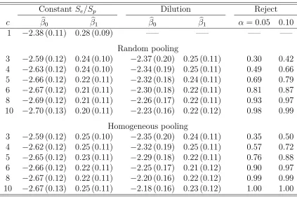
Table 3.4 Irish HBV data analysis with Dorfman decoding. The first-order logistic model in (3.9) is assumed. MLE (estimated standard error) for β= (β0, β1)0 averaged over B = 500 implementations.

“Reject” is the proportion that the likelihood ratio test in Section 3.3 detects dilution using the level of significance α. Individual

testing (c= 1) estimates are also reported for comparison. . . 54

Table A.1 Simulation results under prior misspecification. The true value of p is p = (0.80,0.10,0.09,0.01). The true values of Se:j and

Sp:j are 0.95 and 0.99, respectively. All quantities below are

as defined in Sections 2.4-2.5. The use of “∗” with S_e∗_:_j and S_p∗_:_j

stresses that these are the wrong values. . . 90

Table A.2 Simulation results under prior misspecification. The true value of p is p = (0.95,0.03,0.01,0.01). The true values of Se:j and

Sp:j are 0.95 and 0.99, respectively. All quantities below are

as defined in Sections 2.4-2.5. The use of “∗” with S_e∗_:_j and S_p∗_:_j

(13)

Table A.3 Nebraska CT/NG prevalence estimation results for 2009. Bayesian estimates (Bayes) are posterior medians averaged overB = 500 data sets; BSE is the average of the standard deviations calcu-lated from posterior samples of the B = 500 data sets. Values of a0 = 0, a0 = 0.5, anda0 = 1 are used to incorporate different

amounts of historical information for p as described in Section 2.5. Flat priors forSe:j andSp:j are used, wherej = 1 for CT and

j = 2 for NG; i.e., Se:j ∼ beta(1,1) and Sp:j ∼ beta(1,1).

Max-imum likelihood estimates, calculated from Tebbs et al. (2013), are averaged over the same 500 data sets; the entries under SE

are the averaged standard errors. Stratum sample sizes N are given. 96

Table A.4 Bayesian assay accuracy estimates from 2009. Bayesian esti-mates (Bayes) are posterior medians averaged over B = 500 data sets; BSE is the average of the standard deviations calcu-lated from posterior samples of the B = 500 data sets. Values of a0 = 0, a0 = 0.5, anda0 = 1 are used to incorporate different

amounts of historical information for p as described in Section 2.5. Flat priors for Se:j and Sp:j are used, where j = 1 for CT

and j = 2 for NG; i.e., Se:j ∼beta(1,1) andSp:j ∼beta(1,1). . . . 97

Table B.1 Simulation results for master pool testing (MPT) and Dorfman decoding (DD) withθ = (β0, β1, β2, λ)0 = (−3,2,1, λ)0. “Mean”

is the averaged maximum likelihood estimate and SE is the aver-aged standard error estimate calculated from 500 simulated data sets. Cov is the estimated coverage rate of nominal 95% Wald confidence intervals. The margin of error for the estimated cov-erage rate, assuming a 99% confidence level, is 0.03. Constant pool sizes c are used. Homogeneous pooling has been used for

this simulation. . . 107

Table B.2 Robustness study with misspecified submodels for master pool

testing (MPT) and Dorfman decoding (DD), whereθ = (β0, β1, β2, λ)0 =

(−3,2,1, λ)0. The proposed methods with the assumed submodel in (3.8) are fitted to the group testing data generated using the submodels HS, Probit, and Cloglog. Estimated size and power of the α = 0.05 likelihood ratio test calculated from 500 simu-lated data sets. The margin of error for the estimated size when λ= 0, assuming a 99% confidence level, is 0.03. Constant pool

(14)

Table B.3 Irish HBV data analysis with Dorfman decoding. The polyno-mial logistic model in Equation (3.10) is assumed. MLE (esti-mated standard error) for β = (β0, β1, β2)0 averaged over B =

500 implementations. “Reject” is the proportion that the like-lihood ratio test in Section 3.3 detects dilution using the level of significance α. Individual testing (c = 1) estimates are also

(15)

List of Figures

Figure 2.1 Simulation results with p = (0.80,0.10,0.09,0.01), N = 1000 individuals, Se:j = 0.95, and Sp:j = 0.99, for j = 1,2. The 5th

(bottom), 25th, 50th (median), 75th, and 95th (top) percentiles of the B = 500 posterior median estimates of p are provided. Flat priors forSe:j and Sp:j are used; i.e., Se:j ∼beta(1,1) and

Sp:j ∼beta(1,1). The precision parameter a0 increases from 0

(no historical information aboutpprovided) to 1 by increments

of 0.1. . . 21

Figure 2.2 Simulation results with p = (0.80,0.10,0.09,0.01), N = 1000 individuals, Se:j = 0.95, and Sp:j = 0.99, for j = 1,2. The 5th

(bottom), 25th, 50th (median), 75th, and 95th (top) percentiles of the B = 500 posterior median estimates of Se:j and Sp:j are

provided. Flat priors for Se:j and Sp:j are used; i.e., Se:j ∼

beta(1,1) and Sp:j ∼ beta(1,1). The precision parameter a0

increases from 0 (no historical information about p provided)

to 1 by increments of 0.1. . . 22

Figure 3.1 Irish HBV data analysis with Dorfman decoding and random pooling. The first-order logistic model in (3.9) is assumed. Esti-mated regression functions, averaged over B = 500 implemen-tations, are presented. The estimated regression function for

individual testing is also shown for comparison. . . 52

Figure 3.2 Irish HBV data analysis with Dorfman decoding and random pooling. The polynomial logistic model in (3.10) is assumed. Estimated regression functions, averaged over B = 500 imple-mentations, are presented. The estimated regression function

(16)

Figure A.1 Simulation results with p = (0.80,0.10,0.09,0.01), N = 1000 individuals, Se:j = 0.95, and Sp:j = 0.99, for j = 1,2. The 5th

of 0.1. . . 80

Figure A.3 Simulation results with p = (0.80,0.10,0.09,0.01), N = 1000 individuals, Se:j = 0.95, and Sp:j = 0.99, for j = 1,2. The

5th (bottom), 25th, 50th (median), 75th, and 95th (top) per-centiles of the B = 500 posterior median estimates of p are provided. Informative priors for Se:j and Sp:j are used; i.e.,

Se:j ∼ beta(109.0,6.7) and Sp:j ∼ beta(55.2,1.6). The

preci-sion parameter a0 increases from 0 (no historical information

about p provided) to 1 by increments of 0.1. . . 82

provided. Informative priors for Se:j and Sp:j are used; i.e.,

Se:j ∼beta(109.0,6.7) andSp:j ∼beta(55.2,1.6). The precision

parametera0 increases from 0 (no historical information about

p provided) to 1 by increments of 0.1. . . 83

(17)

Figure A.7 Simulation results with p = (0.95,0.03,0.01,0.01), N = 1000 individuals, Se:j = 0.95, and Sp:j = 0.99, for j = 1,2. The

5th (bottom), 25th, 50th (median), 75th, and 95th (top) per-centiles of the B = 500 posterior median estimates of p are provided. Informative priors for Se:j and Sp:j are used; i.e.,

Se:j ∼ beta(109.0,6.7) and Sp:j ∼ beta(55.2,1.6). The

preci-sion parameter a0 increases from 0 (no historical information

about p provided) to 1 by increments of 0.1. . . 86

provided. Informative priors for Se:j and Sp:j are used; i.e.,

Se:j ∼beta(109.0,6.7) andSp:j ∼beta(55.2,1.6). The precision

parametera0 increases from 0 (no historical information about

p provided) to 1 by increments of 0.1. . . 87

Figure B.1 Robustness study with misspecified submodel using random pooling and moderate misclassification. Boxplots of the maximum likelihood estimates for β = (β0, β1, β2)0 from 500

simulated data sets are presented. The proposed method with the submodel in Equation (3.8) is fit to group testing data gen-erated using the submodel ‘HS’. On the horizontal axes, ‘I’ refers to individual testing, ‘C’ refers to the constantSe/Sp method,

and ‘D’ refers to our proposed dilution method. Constant pool sizes c are reported in parentheses. The true parameter values

(18)

Figure B.2 Robustness study with misspecified submodel using homoge-neous pooling and moderate misclassification. Boxplots of the maximum likelihood estimates forβ = (β0, β1, β2)0 from

500 simulated data sets are presented. The proposed model with the submodel in (3.8) is fit to the group testing data gen-erated using the submodel ‘HS’. On the horizontal axes, ‘I’ refers to individual testing, ‘C’ refers to the constantSe/Sp method,

are represented by dashed horizontal lines. . . 110

simulated data sets are presented. The proposed model with the submodel in (3.8) is fit to the group testing data generated using the submodel ‘Probit’. On the horizontal axes, ‘I’ refers to individual testing, ‘C’ refers to the constantSe/Sp method,

500 simulated data sets are presented. The proposed model with the submodel in (3.8) is fit to the group testing data gen-erated using the submodel ‘Probit’. On the horizontal axes, ‘I’ refers to individual testing, ‘C’ refers to the constant Se/Sp

method, and ‘D’ refers to our proposed dilution method. Con-stant pool sizescare reported in parentheses. The true

param-eter values are represented by dashed horizontal lines. . . 112

simulated data sets are presented. The proposed model with the submodel in (3.8) is fit to the group testing data generated using the submodel ‘Cloglog’. On the horizontal axes, ‘I’ refers to individual testing, ‘C’ refers to the constantSe/Sp method,

(19)

500 simulated data sets are presented. The proposed model with the submodel in (3.8) is fit to the group testing data gen-erated using the submodel ‘Cloglog’. On the horizontal axes, ‘I’ refers to individual testing, ‘C’ refers to the constant Se/Sp

method, and ‘D’ refers to our proposed dilution method. Con-stant pool sizescare reported in parentheses. The true

param-eter values are represented by dashed horizontal lines. . . 114

Figure B.7 Robustness study with misspecified submodel using random pooling and severe misclassification. Boxplots of the max-imum likelihood estimates for β = (β0, β1, β2)0 from 500

sim-ulated data sets are presented. The proposed model with the submodel in (3.8) is fit to the group testing data generated using the submodel ‘HS’. On the horizontal axes, ‘I’ refers to individual testing, ‘C’ refers to the constantSe/Sp method, and

‘D’ refers to our proposed dilution method. Constant pool sizes c are reported in parentheses. The true parameter values are

represented by dashed horizontal lines. . . 115

Figure B.8 Robustness study with misspecified submodel using homoge-neous pooling and severe misclassification. Boxplots of the maximum likelihood estimates for β = (β0, β1, β2)0 from

500 simulated data sets are presented. The proposed model with the submodel in (3.8) is fit to the group testing data gen-erated using the submodel ‘HS’. On the horizontal axes, ‘I’ refers to individual testing, ‘C’ refers to the constantSe/Sp method,

sim-ulated data sets are presented. The proposed model with the submodel in (3.8) is fit to the group testing data generated us-ing the submodel ‘Probit’. On the horizontal axes, ‘I’ refers to individual testing, ‘C’ refers to the constantSe/Sp method, and

‘D’ refers to our proposed dilution method. Constant pool sizes c are reported in parentheses. The true parameter values are

(20)

Figure B.10 Robustness study with misspecified submodel using homoge-neous poolingandsevere misclassification. Boxplots of the maximum likelihood estimates for β = (β0, β1, β2)0 from 500

simulated data sets are presented. The proposed model with the submodel in (3.8) is fit to the group testing data generated using the submodel ‘Probit’. On the horizontal axes, ‘I’ refers to individual testing, ‘C’ refers to the constantSe/Sp method,

sim-ulated data sets are presented. The proposed model with the submodel in (3.8) is fit to the group testing data generated us-ing the submodel ‘Cloglog’. On the horizontal axes, ‘I’ refers to individual testing, ‘C’ refers to the constantSe/Sp method,

Figure B.12 Robustness study with misspecified submodel using homoge-neous poolingandsevere misclassification. Boxplots of the maximum likelihood estimates for β = (β0, β1, β2)0 from 500

simulated data sets are presented. The proposed model with the submodel in (3.8) is fit to the group testing data generated using the submodel ‘Cloglog’. On the horizontal axes, ‘I’ refers to individual testing, ‘C’ refers to the constantSe/Sp method,

Figure B.13 Irish HBV data analysis with Dorfman decoding and homo-geneous pooling. The first-order logistic model in Equation (3.9) is assumed. Estimated regression functions, averaged over B = 500 implementations, are presented. The estimated

regres-sion function for individual testing is also shown for comparison. . 123

Figure B.14 Irish HBV data analysis with Dorfman decoding and homo-geneous pooling. The polynomial logistic model in Equation (3.10) is assumed. Estimated regression functions, averaged over B = 500 implementations, are presented. The estimated regression function for individual testing is also shown for

(21)

Chapter 1 Introduction

1.1 Literature review

We start with a brief literature review of group testing classification (case

identifica-tion) and estimation problems. Before starting our main discussion, we define two

accuracy measures of a diagnostic assay that are associated with group testing. The

sensitivity is the probability that a positive sample is diagnosed as positive, and the

specificity is the probability that a negative sample is diagnosed as negative. In a

multiple-infection problem, we define these accuracy measures for each infection

sep-arately (see Chapter 2). To capture pooled dilution effects, we model the sensitivity

in Chapter 3 as an increasing function of the number of true positives within a pool.

Background

With the goal of minimizing testing costs, Dorfman (1943) introduced the idea of

group testing to screen US soldiers for syphilis during the Second World War.

Dorf-man’s method, which is commonly referred to as “Dorfman testing,” is a two-stage

hierarchical algorithm where initial (non-overlapping) master pools are tested in stage

1 and then individual retesting is performed in stage 2. If a pool is diagnosed as

neg-ative, all individuals in the pool are declared negative; on the other hand, if a pool is

diagnosed as positive, all individuals in the pool are retested one-by-one. As

demon-strated by Dorfman, this simple two-stage algorithm can offer substantial savings in

(22)

testing has been widely accepted as a cost-effective alternative to individual testing

in many applications, including public health, genetics, animal disease testing, drug

discovery, and pollution detection.

Classification

The use of Dorfman’s two-stage procedure has been well regarded by both

practi-tioners and researchers. The popularity of this method can likely be explained by

the fact that it is simple to implement. Many variations of Dorfman’s algorithm are

currently available. For example, Pilcher et al. (2005) uses a three-stage algorithm

which involves a second stage of testing subpools if the master pool tests positively.

Halving algorithm (Litvak et al., 1994) involves multiple stages in which each pool

that tests positively is split further into two halves before testing is performed in

subsequent stages. The final stage of halving involves individual testing.

Unlike hierarchical algorithms, non-hierarchical algorithms use overlapping pools.

An example of a non-hierarchical algorithm is square array testing (Phatarfod and

Sudbury, 1994; Kim et al., 2007). Before performing initial tests, n2 _{specimens are}

placed in an n×n matrix. Then n pools are formed by taking samples from n rows and, similarly, another n pools are created from samples of n columns. These 2n pools are then tested. Specimens at the intersection of a positive row and a positive

column are tested individually. A more generalized square array testing algorithm

allows for the possibility of testing errors. Kim et al. (2007) summarizes the operating

characteristics (i.e., classification efficiency and accuracy) of hierarchical and square

array testing algorithms in the presence of testing error.

Sterrett (1957) proposed an extension of Dorfman’s procedure whereby individuals

from positive pools are retested in multiple stages. According to this procedure,

individuals in a positive pool are tested one-by-one with random selection until the

(23)

a new pool. If the new pool tests negatively, all individuals are declared negative;

however, if the new pool tests positively, individuals in the new pool are again tested

randomly until the first positive one is identified. This procedure is repeated until all

subjects are classified as positive or negative. Sterrett’s decoding procedure can be

more efficient than Dorfman’s when the probability of infection is small.

Sterrett’s procedure has been improved upon by Bilder et al. (2010) who used

individuals’ covariate information to perform informative retesting. In this approach,

each individual’s likelihood of disease positivity is first estimated using covariate

in-formation. When individuals from positive pools are to be retested, an individual who

is most likely to be positive is tested first. Motivated by this informative approach,

McMahan et al. (2012a) generalized array testing to account for the heterogeneity

among individuals. McMahan et al. (2012b) suggested an informative version of

Dorfman decoding in which pools are formed based on individuals’ risk

probabili-ties. Informative approaches can be significantly more efficient when compared to

the corresponding non-informative approaches; i.e., those that do not account for

heterogeneity among individuals.

As testing for multiple infections is becoming more common, group testing

re-search is also shifting. This is because recently developed assays can accurately detect

multiple infections simultaneously from a single specimen. Tebbs et al. (2013) first

studied a two-stage Dorfman-type testing protocol adopted by the Infertility

Preven-tion Project (IPP) for chlamydia and gonorrhea testing. These authors demonstrated

that efficiency can be increased dramatically when pool testing involves multiple

in-fections. The findings presented in Tebbs et al. (2013) serve as motivation to extend

existing classification algorithms from single to multiple infections. Further

advance-ments can be possible when exploiting heterogeneity among individuals as proposed

(24)

Estimation

While group testing research for classification has flourished over the past decades,

estimation has also received substantial attention. Testing data obtained from any

group testing protocol, such as Dorfman decoding, halving, and array testing, can be

modeled to estimate either an overall disease prevalence or individual-level disease

probabilities using covariates. For a rare disease, inference based on group testing

can be as efficient as that for individual testing at only a fraction of the testing cost.

Even though retesting individuals from positive pools is necessary for classification

purposes, retesting is not crucial for estimation. This can be explained heuristically as

follows. If a disease is rare, pools that test positively may not contain more than one

positive case; hence, retesting individuals from positive pools provides little additional

information. Therefore, the majority of group testing papers that proposed estimation

methods used testing responses from only initial master pools. The advantages of

this approach include simplicity in statistical modeling and additional reductions in

testing costs.

Most researchers in group testing, until the late 1990’s, focused only on estimating

the proportion (overall prevalence) of a rare binary trait. The first such estimation

paper is Thompson (1962), who took a maximum likelihood (ML) approach to

esti-mate the proportion of insect vectors capable of transmitting aster-yellow virus in a

population of aphids. Thompson’s work proceeded under the assumption that testing

results are perfect and that insects’ infection statuses are independent. In addition

to using master pool responses as in Thompson (1962), Sobel and Elashoff (1975)

al-lowed the statistical model to incorporate retest information. Hwang (1976) proposed

a maximum likelihood estimator (MLE) in the presence of dilution effects. Burrows

(1987) took an alternative ML approach which can improve estimation in terms of

bias and efficiency. Robustness of estimation has been studied by several authors

(25)

authors have studied group testing optimality; among others, see Tu et al. (1995)

and Liu et al. (2012).

Group testing estimation from within a Bayesian paradigm has also been studied.

Chaubey and Li (1995) presented a Bayesian method for estimation and showed that

Bayesian estimators can be preferred to ML estimators. Mendoza-Blanco et al. (1996)

presented a general Bayesian framework that models data resulting from a variety of

sampling strategies. Bilder and Tebbs (2005) proposed an empirical Bayes method

for estimation using master pools only. Johnson and Pearson (1999) developed a

Bayesian methodology for a two-stage testing where individuals from pools that test

negatively are re-pooled. This technique was originally proposed by Gastwirth and

Johnson (1994) who took a frequentist approach. A similar method was proposed

by Hanson et al. (2006), who acknowledge heterogeneity among populations due to

regional differences and allow the model to incorporate varying prevalences.

With the exception of Hanson et al. (2006), all of the estimation methods discussed

above aim at estimating a single proportion without accounting for heterogeneity

among individuals. Recent work has focused on developing regression methodology

using covariates, such as age, gender, and disease symptoms, to obtain

individual-level estimates. Farrington (1992) first proposed a regression method for a specific

generalized linear model with the stringent assumption that each individual within

a pool shares identical covariates. Vansteelandt et al. (2000) extended this work to

allow for any type of covariate structure. Xie (2001) presented a general

expectation-maximization methodology which can incorporate retest results. Bilder and Tebbs

(2009) studied estimation bias and efficiency for regression estimates using the model

introduced by Vansteelandt et al. (2000). Huang and Tebbs (2009) and Huang (2009)

developed diagnostic methods to identify latent model misspecification for structural

measurement error models using group testing responses. McMahan et al. (2013)

(26)

(2015) generalized the regression method of McMahan et al. (2013) to be applicable

for any group testing algorithm.

A number of papers have presented nonparametric regression estimation

meth-ods for group testing data. The seminal work in Delaigle and Meister (2011) used

test results from randomly formed pools. Delaigle and Hall (2012) later presented

a nonparametric approach for pools formed homogeneously. Wang et al. (2014b)

presented a general semiparametric approach to model data from any group testing

algorithm. Delaigle and Zhou (2015) presented a nonparametric extension of the

dilution methods in McMahan et al. (2013).

Switching gears to multiple infections, Hughes-Oliver and Rosenberger (2000) first

proposed a method to estimate the prevalence of multiple diseases with the

assump-tion that a perfect assay test is available to detect all diseases simultaneously. Tebbs

et al. (2013) extended this work to allow for imperfect testing and to incorporate

in-dividual retest results. Zhang et al. (2013) proposed a regression method for multiple

diseases. The research direction of group testing with multiple diseases is becoming

popular because of its additional cost savings and also because of the availability of

multiple-infection assays.

Subsequent chapters of this dissertation are organized as follows. In Chapter 2,

we present a Bayesian model to estimate the prevalence of multiple infections. In

Chapter 3, we present a regression method for single traits that accounts for dilution.

In Chapter 4, we propose a Bayesian framework that corrects for measurement errors

in covariates. Finally, we describe future research ideas in Chapter 5. Supplementary

(27)

Chapter 2 Estimating the prevalence of multiple diseases

from two-stage hierarchical pooling

1

The material in this chapter and Appendix A are taken from the manuscript,

“Esti-mating the prevalence of multiple diseases from two-stage hierarchical pooling,” by

M. Warasi, J. Tebbs, C. McMahan, and C. Bilder. This manuscript was accepted at

Statistics in Medicineon 03/17/2016. Permission to reprint is shown in Appendix C.

Summary: Testing protocols in large-scale sexually transmitted disease screening

applications often involve pooling biospecimens (e.g., blood, urine, swabs, etc.) to

lower costs and to increase the number of individuals who can be tested. With the

recent development of assays that detect multiple diseases, it is now common to test

biospecimen pools for multiple infections simultaneously. Recent work has developed

an expectation-maximization algorithm to estimate the prevalence of two infections

using a two-stage, Dorfman-type testing algorithm motivated by current screening

practices for chlamydia and gonorrhea in the United States. In this article, we have

the same goal but instead take a more flexible Bayesian approach. Doing so allows

us to incorporate information about assay uncertainty during the testing process,

which involves testing both pools and individuals, and also to update information as

individuals are tested. Overall, our approach provides reliable inference for disease

probabilities and accurately estimates assay sensitivity and specificity even when little

1_{Warasi, M., Tebbs, J., McMahan, C., and Bilder, C. (2016).} _{Estimating the prevalence}

(28)

or no information is provided in the prior distributions. We illustrate the performance

of our estimation methods using simulation and by applying them to chlamydia and

gonorrhea data collected in Nebraska.

2.1 Introduction

Testing biospecimens in pools, which is known as group testing (or pooled testing),

is a cost-effective alternative to individual testing in a variety of disease screening

applications. Originally proposed by Dorfman (1943) to screen World War II soldiers

for syphilis, group testing is now widely used to screen human populations for sexually

transmitted diseases, including HIV (Pilcher et al., 2005), HBV and HCV (Hourfar

et al., 2008; Stramer et al., 2013), and chlamydia and gonorrhea (Lindan et al., 2005),

and for other infectious diseases including West Nile virus (Busch et al., 2005), malaria

(Wang et al., 2014a), and influenza (Van et al., 2012). Group testing also arises in

other applications, including drug discovery (Remlinger et al., 2006), genetics (Chi

et al., 2009), animal disease testing (Dhand et al., 2010), and food safety (Fahey

et al., 2006).

Because pooling has become so widespread, statistical research in group testing

has also flourished. This research has generally followed two different paths. In

the classification (case identification) problem, the goal is to classify each

individ-ual as positive or negative. This involves retesting individindivid-uals in pools that test

positively; see Kim et al. (2007) for a review. In the estimation problem, responses

from pools provide enough information to estimate a population prevalence, at times,

more efficiently than when individual testing is used (Liu et al., 2012; Zhang et al.,

2013). Recent work has focused on the development of regression methods to

esti-mate subject-specific probabilities, either parametrically (Vansteelandt et al., 2000;

Chen et al., 2009), semi-parametrically (Wang et al., 2014b), or non-parametrically

(29)

This article is motivated by screening practices for chlamydia and gonorrhea

(CT/NG) in the United States as part of a national program formerly known as

the Infertility Prevention Project (IPP). Chlamydia and gonorrhea are two of the

most common sexually transmitted diseases; together, there are approximately 1.5

million new infections reported each year in the United States (Gaydos et al., 2010).

The IPP was a federally funded program managed by the Centers for Disease Control

and Prevention (CDC) and implemented in each of the 50 states during 1988-2013.

After the Affordable Care Act (ACA) was passed in 2010 and implemented in 2014,

screening for CT/NG has continued in each state but now testing centers rely on

other sources of funding (e.g., federal health care plans, private insurance, etc.). To

reduce costs while still screening the same number of individuals for CT/NG, Iowa’s

IPP program switched from individual testing to group testing in 1999. Doing so has

led to millions of dollars in savings (Jirsa, 2008), and other states (Lewis et al., 2012)

have since adopted group testing as well. In light of new funding uncertainties created

by the ACA (JSI Research & Training Institute, 2015), Iowa’s application of group

testing might serve as a model for how to perform CT/NG screening nationwide.

Estimating the prevalence of a single disease has received a large amount of

at-tention in the group testing literature. However, testing procedures for CT/NG and

other infections are now moving towards the use of assays which detect multiple

infec-tions at once (Gaydos et al., 2010). In these instances, pools of individuals are tested

for multiple infections using a single assay, and then pools are resolved (decoded)

for each infection. Estimation in this situation is challenging, because the true

infec-tion statuses on the same individual are latent (due to inherent assay error) and are

also correlated. Recently, Tebbs et al. (2013) developed an expectation-maximization

(EM) algorithm to jointly estimate the prevalence of CT/NG, motivated by screening

practices in Iowa which use group testing (see Section 2.2). Their work, in the

(30)

(2000) to allow for assay error and also for the inclusion of retesting information on

positive pools.

In this article, we have the same estimation goals as in Tebbs et al. (2013), but

we take a Bayesian approach instead. Doing so confers important advantages. First,

it allows us to relax the potentially untrustworthy assumption that diagnostic test

accuracy rates (i.e., sensitivity and specificity) are fixed and known. In practice, these

rates are usually estimated on the basis of small pilot studies that manufacturers

publish in their product literature. Ignoring the variability in these estimates could

compromise inference, especially if the estimates deviate substantially from the true

accuracy rates and/or if assay performance varies according to other factors (CDC,

2015). Second, a Bayesian approach is natural given the sequential manner in which

screening data amass over time. For example, the State Hygienic Laboratory (SHL)

in Iowa City has screened thousands of Iowa residents each year for CT/NG, dating

back to 1992. This affords investigators ample information to construct sensible prior

distributions as well as to periodically update information on disease prevalence and

assay performance. Our work extends previous Bayesian group testing estimation

approaches for single diseases (Johnson and Pearson, 1999; Hanson et al., 2006).

Subsequent sections of this article are organized as follows. In Section 2.2, we

describe the screening algorithm for CT/NG used in Iowa. This two-stage algorithm

was described in detail in Tebbs et al. (2013), so we herein summarize only the salient

aspects. In Section 2.3, we present our estimation methods and discuss prior model

selection. In Section 2.4, we use simulation to assess estimation performance under a

variety of prior models, including models which incorporate little or no information

about disease prevalence and assay accuracy. In Section 2.5, we analyze IPP data in

the same manner as in Tebbs et al. (2013) to illustrate the advantages of estimation

from a Bayesian point of view. In Section 2.6, we conclude with a brief summary

(31)

probabilities for more than two infections if needed.

2.2 Two-stage pooling algorithm

The estimation methods we develop in this article are motivated by the two-stage

pooling algorithm described below. This algorithm is used to complete CT/NG

test-ing at the SHL in Iowa City and is potentially applicable in other situations.

POOLING ALGORITHM

Stage 1: Individuals are randomly assigned to master pools. Each pool is tested for

both infections using a single assay. A single assay detects both infections

simulta-neously.

Stage 2: Individuals in pools that

• test negatively for both infections are diagnosed as negative for both infections.

• test positively for either infection are retested (individually) for both infections using the same assay in Stage 1. Diagnoses for both infections are made from

the outcomes of the individual tests.

Tebbs et al. (2013) describe various logistical issues of this pooling procedure (as it

relates to implementation at the SHL) that we do not repeat here. The point worth

emphasizing is that, for simplicity, the SHL uses one assay, the Aptima Combo 2

Assay (Hologic/Gen-Probe, Inc., San Diego) nucleic acid amplification test, for its

CT/NG testing. This assay detects both infections simultaneously when it is applied

to pools (in Stage 1) and to individuals (in Stage 2). In the infectious disease testing

literature, such an assay is said todiscriminate because it elicits a diagnosis for each

infection separately. In this article, we assume that a discriminating assay is available

and that it can be applied to both pooled and individual specimens. The literature is

(32)

For example, most assays based on nucleic acid amplification technology used for

CT/NG detection discriminate between the two infections in both urine and swab

specimens (Gaydos et al., 2010; CDC, 2015). Furthermore, the CDC recommends

that nucleic acid amplification testing be used for laboratory-based CT/NG detection

(CDC, 2015).

2.3 Bayesian estimation

Model formulation and inference

Suppose N individuals are to be tested for two infections (e.g., CT/NG, etc.) using the algorithm described in Section 2.2. Let fY_ik = (Ye_i₁_k,Ye_i₂_k)0 denote the vector

of true individual binary statuses, for i = 1,2, ..., ck and k = 1,2, ..., K, where N =

PK

k=1ck. We callckthe pool size for thekth master pool. The number of master pools

formed at Stage 1 is K. We assume the Yf_ik’s, conditional on p= (p₀₀, p₁₀, p₀₁, p₁₁)0,

are independent and identically distributed random vectors with probability mass

function

pr(Ye_i₁_k = e

y1,Ye_i₂_k= e

y2|p) =p (1−

e

y1)(1−_ey2)

00 pe

y1(1−_ey2)

10 p

(1− e

y1)_ey2

01 pe

y1ey2

11 ,

where ye1,ye2 ∈ {0,1} and p00 +p10+p01 +p11 = 1. Note that because of inherent

assay error, the fY_ik’s are best regarded as latent.

Let Ze_k = (Ze₁_k,Ze₂_k)0 denote the vector of true binary statuses for the kth master

pool, whereZe_jk =I(Pc_i₌₁k Ye_ijk>0), forj = 1,2, and I(·) is the indicator function. In

other words, Ze_jk = 1 if at least one individual in the kth master pool is truly positive

for the jth infection, Ze_jk = 0 otherwise. Let Z_k = (Z₁_k, Z₂_k)0 denote the vector of

testing responses observed for the kth master pool in Stage 1, where Zjk = 1 if the

kth master pool tests positively for the jth infection, Zjk = 0 otherwise. If the kth

master pool tests positively for at least one infection in Stage 1, letYik = (Yi1k, Yi2k)0

(33)

i = 1,2, ..., ck, in Stage 2. We allow for pools (in Stage 1) and individuals (in Stage

2) to be misclassified and denote the assay sensitivity and specificity by

Se:j = pr(Zjk = 1|Ze_jk = 1) = pr(Y_ijk = 1|Ye_ijk = 1)

Sp:j = pr(Zjk = 0|Ze_jk = 0) = pr(Y_ijk = 0|Ye_ijk = 0),

respectively, forj = 1,2. We assumeSe:j andSp:j do not depend on the pool sizeckin

Stage 1 so that these probabilities also apply for individual tests performed in Stage

2. This assumption is common in group testing research for single infections (Kim

et al., 2007). For this to be reasonable in practice, assay detection thresholds and/or

dilution ratios may need to be changed to accommodate both pooled and individual

specimens; see McMahan et al. (2013) and the references therein.

The observed data from the pooling algorithm in Section 2.2 consist of (a) the

test-ing responses Zk = (Z1k, Z2k)0 from the K master pools in Stage 1 and (b) the

addi-tionalck individual testing responsesYik = (Yi1k, Yi2k)0 from those pools which tested

positively for either infection in Stage 1. For notational purposes, we aggregate all

master pool testing responses into a vector denoted byZand all individual testing

re-sponses into a vector denoted byY. Letθ= (p0,δ0)0, whereδ = (Se:1, Se:2, Sp:1, Sp:2)0.

Although it is possible to write out the observed data likelihoodπ(Z,Y|θ), its form is not easily amenable to performing a Bayesian analysis. Therefore, we use a data

aug-mentation step that introduces the individuals’ true infection statuses Ye_ijk as latent

random variables. Let fY denote the vector that aggregates all of the latent Ye_ijk’s.

(34)

onθ, can be expressed as

π(Z,Y,fY|θ) =

K

Y

k=1

ck Y

i=1

p(1−Yei1k)(1−Yei2k)

00 pe

Yi1k(1−Yei2k)

10 p

(1−Y_ei1k)Yei2k

01 pe

Yi1kYei2k 11

×





2

Y

j=1

K

Y

k=1

SZjk

e:j S

1−Zjk

e:j

I(Pck_i₌₁Yeijk>0)

S1−Zjk

p:j S Zjk

p:j

I(Pck_i₌₁Yeijk=0)

×

(_c_k

Y

i=1

SYijkYeijk

e:j S

(1−Yijk)Yeijk

e:j S

(1−Yijk)(1−Yeijk)

p:j S

Yijk(1−Yeijk)

p:j

)I(Z+k>0) 

, (2.1)

where Z+k = Z1k +Z2k, Se:j = 1− Se:j, and Sp:j = 1− Sp:j. The first line in

Equation (2.1) represents the contribution of the individual latent statuses, while the

part within the brackets describes the contributions from Stage 1 (master pool test

results; second line) and Stage 2 (individual test results; third line). Note that if δ

were known, Equation (2.1) would be the same as the complete data likelihood in

Tebbs et al. (2013). For further discussion on additional assumptions underpinning

the construction of π(Z,Y,fY|θ) in Equation (2.1), see Section 2.6.

To complete our Bayesian model specification, we elicit independent beta prior

distributions for the assay test accuracies; i.e., Se:j ∼ beta(aSe:j, bSe:j) and Sp:j ∼

beta(aSp:j, bSp:j), for j = 1,2, where all hyperparameters are known. For the vector

of infection status probabilities, we specify a Dirichlet prior; i.e.,

p∼π(p) =B(α)pα00−1

00 p

α10−1

10 p

α01−1

01 p

α11−1

11 ,

whereB(α) is a normalizing constant andα= (α00, α10, α01, α11)0is a vector of known

hyperparameters. We assume the test accuracies Se:j and Sp:j are both independent

(35)

With these prior choices and assumptions, the “full conditional” distributions can

be easily derived from the augmented likelihood functionπ(Z,Y,fY|θ). For the assay

accuracies, these distributions are given by

Se:j|Z,Y,fY ∼ beta(a∗_S e:j, b

∗

Se:j)

Sp:j|Z,Y,fY ∼ beta(a∗

Sp:j, b ∗

Sp:j),

for j = 1,2, where

a∗_S

e:j = aSe:j +

K

X

k=1

(

ZjkZe_jk +I(Z₊_k >0)

ck X

i=1

YijkYe_ijk )

b∗_S

e:j = bSe:j+

K

X

k=1

(

(1−Zjk)Ze_jk+I(Z₊_k >0)

ck X

i=1

(1−Yijk)Ye_ijk )

a∗_S

p:j = aSp:j+

K

X

k=1

(

(1−Zjk)(1−Ze_jk) +I(Z₊_k>0)

ck X

i=1

(1−Yijk)(1−Ye_ijk) )

b∗_S_p_:_j = bSp:j +

K

X

k=1

(

Zjk(1−Ze_jk) +I(Z₊_k >0)

ck X

i=1

Yijk(1−Ye_ijk) )

and Ze_jk = I(Pc_i₌₁k Ye_ijk > 0). For the prevalence parameter p, the full conditional

distribution is again Dirichlet; i.e., p|fY∼Dirichlet(Ψ), where

Ψ=



α₀₀+

K X k=1 ck X i=1 e

V(00)ik, α10+

K X k=1 ck X i=1 e

V(10)ik,

α01+

K X k=1 ck X i=1 e

V(01)ik, α11+

K X k=1 ck X i=1 e

V(11)ik



 0

and the latent random variablesVe₍_uv₎_ik =Ye_iu

1k(1−Ye_i₁_k)1−uYe_iv

2k(1−Ye_i₂_k)1−v, for u, v ∈

{0,1}.

If the latent data Yf were observed, the posterior distributions for the prevalence

parameters in p and the test accuracies in δ would be fully determined. However,

because the true individual statuses in fY are not observed, we develop a Gibbs

sampler to enable posterior inference. Let fY_k₍_i₎ = (fY0

1k, ...,Yf

0

i−1,k,Yf

0

i+1,k, ...,fY

0

ckk) 0

(36)

{fY_k₍_i₎,p,δ,Y,Z} is multinomial with cell probabilities ζ₀₀ik/ζik, ζ₁₀ik/ζik, ζ₀₁ik/ζik, and

ζik

11/ζik, where

ζ₀₀ik =p00 2

Y

j=1

SZjk

e:j S

1−Zjk

e:j

γijk

S1−Zjk

p:j S Zjk

p:j

1−γijk

S1−Yijk

p:j S Yijk

p:j

I(Z+k>0)

ζ₁₀ik =p10SeZ:11kS 1−Z1k

e:1

SZ2k

e:2 S 1−Z2k

e:2

γi2k

S1−Z2k

p:2 S

Z2k

p:2

1−γi2k

×SYi1k

e:1 S 1−Yi1k

e:1 S 1−Yi2k

p:2 S

Yi2k

p:2

I(Z+k>0)

ζ₀₁ik =p01SeZ:22kS 1−Z2k

e:2

SZ1k

e:1 S 1−Z1k

e:1

γi1k

S1−Z1k

p:1 S

Z1k

p:1

1−γi1k

×SYi2k

e:2 S 1−Yi2k

e:2 S 1−Yi1k

p:1 S

Yi1k

p:1

I(Z+k>0)

ζ₁₁ik =p11 2

Y

j=1

SZjk

e:j S

1−Zjk

e:j

SYijk

e:j S

1−Yijk

e:j

I(Z+k>0)

,

ζik =P1

u=0

P1

v=0ζuvik, and γijk =I(Pi0₆₌_iYe_i0_jk >0). Note that by sampling fV_ik from

this conditional distribution, fY_ik = (Ve₍₁₀₎_ik+Ve₍₁₁₎_ik,Ve₍₀₁₎_ik+Ve₍₁₁₎_ik)0; in other words,

the true individual statuses in fY_ik are uniquely determined.

Using the full conditional distributions of p, δ, and fV_ik described above, we now

outline our Gibbs sampler to implement a Bayesian analysis with the observed data

from the pooling algorithm described in Section 2.2:

GIBBS SAMPLER

1. Initialize Yf(0)_ik = (Ye_i(0)

1k,Ye_i(0)

2k)0, for i= 1,2, ..., ck and k= 1,2, ..., K. Set d= 1.

2. Sample p(d) _from_p_|

f

Y(d−1) _∼_Dirichlet(_Ψ_{), where}

f

Y(d−1) _{is the collection of all}

f

Y(_ikd−1)’s.

3. Sample S_e(d_:_j) from Se:j|Z,Y,fY(d−1) ∼ beta(a∗_S e:j, b

∗

Se:j) and sample S (d)

p:j from

Sp:j|Z,Y,Yf(d−1) ∼beta(a∗_S p:j, b

∗

Sp:j) forj = 1,2. Setδ

(d)_{= (}_S(d)

e:1, S (d)

e:2, S (d)

p:1, S (d)

p:2)0.

4. Fori= 1, ..., ck andk = 1,2, ..., K, samplefV(d)

ik = (Ve

(d) (00)ik,Ve

(d) (10)ik,Ve

(d) (01)ik,Ve

(d) (11)ik)

0

from

f

Vik|fY(d)

k(i),p

(d)_,_δ(d)_,_Y_,_Z_∼_multinomialn₁_,₍_ζik

00/ζ

ik_{, ζ}ik

10/ζ

ik_{, ζ}ik

01/ζ

ik_{, ζ}ik

11/ζ

ik₎0o

Measuring Strategic Communications

University of South Carolina

Scholar Commons

Modern Estimation Problems in Group Testing

Md Shamim Sarker

Dedication

Acknowledgments

Abstract

Table of Contents

List of Tables

List of Figures

Chapter 1

Introduction

Background

Classification

Estimation

Chapter 2

Estimating the prevalence of multiple diseases

from two-stage hierarchical pooling

Model formulation and inference