HIGHLIGHTED ARTICLE
| INVESTIGATION
Ef
fi
cient Genome-Wide Sequencing and
Low-Coverage Pedigree Analysis from
Noninvasively Collected Samples
Noah Snyder-Mackler,* William H. Majoros,†Michael L. Yuan,* Amanda O. Shaver,* Jacob B. Gordon,‡ Gisela H. Kopp,§,**,††Stephen A. Schlebusch,‡‡Jeffrey D. Wall,§§Susan C. Alberts,*,‡,*** Sayan Mukherjee,†††,‡‡‡,§§§Xiang Zhou,****,††††,1and Jenny Tung*,‡,***,‡‡‡‡,1
*Department of Evolutionary Anthropology,†Graduate Program in Computational Biology and Bioinformatics,‡Department of Biology,†††Department of Statistical Science,‡‡‡Department of Mathematics,§§§Department of Computer Science, and‡‡‡‡Duke University Population Research Institute, Duke University, Durham, North Carolina 27708,§Cognitive Ethology Laboratory, German Primate Center, Leibniz Institute for Primate Research, 37077 Göttingen, Germany, **Department of Biology, University of Konstanz, 78457 Konstanz, Germany,††Department of Migration and Immuno-Ecology, Max Planck Institute for Ornithology, 82319 Radolfzell, Germany,‡‡Department of Molecular and Cell Biology, University of Cape Town, 7700 Cape Town, South Africa,§§Institute for Human Genetics, University of California, San Francisco, California 94143, ***Institute of Primate Research, National Museums of Kenya, Nairobi, Kenya, and ****Department of Biostatistics and††††Center for Statistical Genetics, University of Michigan, Ann Arbor, Michigan 48109 ORCID IDs: 0000-0003-3026-6160 (N.S.-M.); 0000-0003-3026-6160 (W.H.M.); 0000-0003-0416-2958 (J.T.)
ABSTRACTResearch on the genetics of natural populations was revolutionized in the 1990s by methods for genotyping noninvasively collected samples. However, these methods have remained largely unchanged for the past 20 years and lag far behind the genomics era. To close this gap, here we report an optimized laboratory protocol for genome-wide capture of endogenous DNA from noninvasively collected samples, coupled with a novel computational approach to reconstruct pedigree links from the resulting low-coverage data. We validated both methods using fecal samples from 62 wild baboons, including 48 from an independently constructed extended pedigree. We enriched fecal-derived DNA samples up to 40-fold for endogenous baboon DNA and reconstructed near-perfect pedigree relationships even with extremely low-coverage sequencing. We anticipate that these methods will be broadly applicable to the many research systems for which only noninvasive samples are available. The lab protocol and software (“WHODAD”) are freely available at www.tung-lab.org/protocols-and-software.html and www.xzlab.org/software.html, respectively.
KEYWORDScapture-based enrichment; noninvasive samples; baboons; paternity analysis; pedigree; genome resequencing
T
HE capacity to generate genetic data from low-quality or noninvasively collected samples,first developed in the 1990s, revolutionized the study of genetics, evolution, behav-ior, and ecology in natural populations. These methodologicaladvances facilitated phylogenetic and phylogeographic anal-yses of difficult-to-sample taxa; helped define the role of admixture in mammalian evolution (Pérezet al.2010; Sacks
et al.2011; Charpentieret al.2012); and enabled theoretical expectations about paternal investment, kin recognition, and reproductive skew to be empirically tested, sometimes for the first time (Buchanet al.2003; Smithet al.2003; Archieet al.
2007; Gottelliet al. 2007). They also yielded important in-sights into the genetic viability and future prospects of threat-ened or endangered populations from which invasive samples are impossible to obtain (Idaghdouret al.2003; Valièreet al.
2003; Nagata et al.2005; Rudnicket al.2007; Mondolet al.
2009). Noninvasive genetic analysis has thus changed the ways Copyright © 2016 by the Genetics Society of America
doi: 10.1534/genetics.116.187492
Manuscript received January 25, 2016; accepted for publication April 18, 2016; published Early Online April 19, 2016.
Available freely online through the author-supported open access option.
Supplemental material is available online atwww.genetics.org/lookup/suppl/doi:10. 1534/genetics.116.187492/-/DC1.
we study population, ecological, and conservation genetics, and we would know far less about many species without it.
However, techniques for noninvasive genetic analysis have changed little in the past 20 years. Collection of genetic data from noninvasively collected tissues (e.g., feces, hair, and urine) continues to be labor intensive, time intensive, and vulnerable to technical artifacts such as allelic dropout and cross-contamination (Gagneux et al. 1997; Taberlet et al.
1999). Further, current methods ultimately yield very small amounts of data by today’s standards. Typical studies geno-type up to several dozen microsatellite loci per individual—a trivial amount compared to the data sets now routinely gen-erated using standard high-throughput sequencing ap-proaches. Thus, while existing methods are sufficient for basic pedigree construction and estimating some population genetic parameters (although usually with substantial uncer-tainty), they are severely underpowered for many other types of analyses (Sabetiet al.2002; Priceet al.2009; Li and Durbin 2011), including any that require local (i.e., gene- or region-specific) information instead of genome-wide averages (Huanget al.2007; Liet al.2007; Sankararaman and Sridhar 2008; Yang et al. 2011; Ma et al. 2014). Further, because noninvasively collected genotype data are most often based on microsatellites, they cannot take advantage of new tools designed specifically for single-nucleotide variants (Purcell
et al.2007; Visscher 2009; Durandet al.2011).
Generating genome-scale data sets from noninvasive sam-ples is challenging for two reasons. First, in many cases, the DNA extracted from these samples is low quality and highly fragmented. Second, it contains large proportions of nonhost DNA. For example, only1% of DNA extracted from fecal-derived samples is endogenous to the donor animal [most is microbial (Perryet al.2010)]. Sequence capture methods, in which synthesized baits are used to enrich for prespecified target sequences from a larger DNA pool (Gnirkeet al.2009), present a potential solution to both of these problems. Be-cause shearing is a required step in library preparation, the problem of working with highly fragmented samples is obvi-ated. Indeed, Perryet al.(2010) were able to use a modified version of sequence capture to target and sequence 1.5 Mb of the chimpanzee genome from fecal-derived DNA, with very low genotyping error rates relative to blood-derived DNA. More recently, Carpenter et al.(2013) reported a method for performing genome-wide sequence capture from low-quality ancient DNA samples, which recapitulate many of the challenges posed by noninvasive samples (e.g., highly fragmented DNA and low proportions of endogenous DNA). However, while considerable investment in single samples often makes sense in ancient DNA studies, the low levels of postcapture enrichment associated with currently available protocols are not cost effective for population studies of non-invasive samples. Substantially higher rates of enrichment, particularly in nonrepetitive regions of the genome, will be essential to overcome this limitation. In addition, compu-tational methods for analyzing the resulting data are also required, especially given that genome-scale sequencing
efforts for such samples are likely to produce low-coverage data. For example, current paternity assignment approaches (Chakrabortyet al.1974; Marshallet al.1998; Kalinowski
et al.2007) were not designed to deal with uncertain geno-types, an inevitable component of analyzing low-coverage sequencing data. Thus, for capture-based methods to be-come broadly accessible, the development of appropriate new computational approaches is also essential.
Here, we report an optimized laboratory protocol for genome-wide capture of endogenous DNA from noninvasively collected samples, combined with a novel computational approach to reconstruct pedigree links from the resulting data (implemented in the program WHODAD). We validate both our laboratory methods and computational tools, using non-invasively collected samples from 54 members of an inten-sively studied wild baboon population in the Amboseli basin of Kenya (Alberts and Altmann 2012). We also demonstrate the generalizability of our methods to noninvasive samples col-lected using different methods from a different baboon spe-cies from West Africa. Our protocol is cost effective, has manageable sample input requirements, yields good capture efficiency for high complexity, nonrepetitive DNA, and mini-mizes the need for extensive PCR amplification. Importantly, we find that genotype data generated from fecal samples closely match data from high-quality blood-derived DNA samples from the same individuals, and provide near-perfect information on pedigree relationships even with extremely low per-sample sequencing coverage (mean = 0.493 ge-nome coverage). Together, these methods will enable popu-lation, conservation, and ecological genetic analyses of natural populations to again take a major leap forward, into the genomic era. At the same time, they will also introduce new systems to the genomics community.
Results
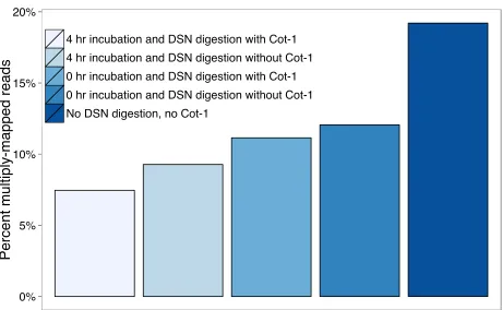
DSN digestion during bait construction increases library complexity
synthesized from low-complexity/highly duplicated regions. Specifically, a 4-hr incubation of sheared DNA at 68°followed by a 20-min DSN digestion in the presence of human Cot-1 produced the highest-complexity bait library of thefive con-ditions we tested. Compared to DNA templates from a non-DSN-digested library, bait templates produced using these conditions reduced the number of reads mapping to multiple locations by 2.6-fold (from 19.2% to 7.5%;Figure S2). Capture-based enrichment
We validated our full capture protocol (bait construction followed by capture of endogenous DNA and sequencing of captured fragments), using fecal-derived DNA (fDNA) sam-ples collected from 54 individually recognized yellow baboons (36 males and 18 females; Figure 1) from the Amboseli ba-boon population, an intensively studied population in which maternal and paternal pedigree relationships are known for a large set of individuals (Buchan et al. 2003; Alberts et al.
2006; Alberts and Altmann 2012). We produced data for 52 of the samples in two successive capture efforts:“capture 1”was conducted on fDNA from 24 baboons, and“capture 2” was conducted on fDNA from 28 additional baboons after making multiple improvements to our initial protocol (changes to the protocol between capture efforts are de-scribed in detail in Table S1andFile S1; seeTable S2 for information on sequencing coverage and mapping statistics). Data from the remaining two individuals,“LIT”and“HAP,” were generated to compare the captured fDNA sample with data derived from sequencing blood-derived genomic DNA (gDNA) samples from the same individuals.
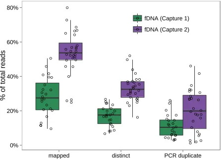
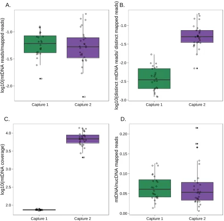
Our protocol (Figure S1) resulted in substantial enrich-ment of baboon DNA in the postcapturevs.precapture sam-ples (see Table S2 for sample-specific details). A mean of 44.56% (range: 10.28–83.17%) of postcapture fragments mapped to the yellow baboon genome (Pcyn1.0), despite starting with precapture samples that contained a mean of only 2.04% endogenous baboon DNA, as estimated by quan-titative PCR (qPCR) (range 0.19–8.37%). However, in cap-ture 1 a large proportion of the mapped fragments were identified as PCR duplicates (meancapture1 = 71.97% of
mapped fragments, rangecapture1 = 51.43–88.46%; Figure
2A). After removing PCR duplicates, a mean of 9.16% of the postcapture reads in capture 1 were nonduplicate map-pable fragments (rangecapture1= 2.23–23.75%), producing a
mean coverage of 0.203per sample relative to the mappable baboon genome (mean sequencing depth of 5.8 Gb per sam-ple; rangecapture1= 0.04–0.493; Figure 2B). These numbers
translated to an overall mean fold enrichment of 39.83for mapped reads (rangecapture1= 8.0–111.8-fold, SD = 25.2)
and 9.63enrichment of non-PCR duplicate mapped reads (rangecapture1= 3.9–22.4-fold, SD = 5.0; Figure 2C).
Based on our results for capture 1, we made multiple protocol improvements prior to conducting capture 2 (Table S1andFile S1). The improved protocol was twice as effective on average, resulting in a mean 18-fold enrichment of high-quality, analysis-ready reads and a maximum fold enrichment
of close to 40-fold [rangecapture2= 8.0–39.2-fold, Figure 2C;
by comparison, methods optimized for ancient DNA achieved a mean of 5.5-fold enrichment of non-PCR duplicate frag-ments (Carpenter et al.2013), Figure 2A]. Specifically, the protocol changes improved the proportion of nonduplicate mapped fragments by .4-fold, from a mean proportion of 9.16% in capture 1 to a mean proportion of 37.74% in cap-ture 2 (rangecapture2= 6.16–68.61%), and reduced the
pro-portion of PCR duplicates among mapped reads 2-fold (from 71.97% in capture 1 to 36.97% in capture 2). This improve-ment translated to an increase in overall genomic coverage from a mean of 0.203in capture 1 to 0.733in capture 2 (mean total sequencing of 5.7 Gb per sample; rangecapture2=
0.19–1.243; Figure 2B). This improvement in coverage was not explained by increased sequencing depth in capture 2 (Table S2). Thus, while we would need to sequence a pre-capture fDNA sample 50–100 times as deeply as a blood- or tissue-derived sample to produce the same level of coverage, our capture method reduces this difference to2 times the sequencing effort. Importantly, our method was also success-ful in enriching fDNA samples (n = 8) from independent samples collected from Guinea baboons (Papio papio; Figure 2A,Table S2), suggesting that our results are highly gener-alizable across different species and storage and extraction methods.
Sample attributes influencing capture efficiency
The amount of baboon DNA in the precapture fDNA sample was the strongest predictor of enrichment success. Specifi -cally, the percentage of baboon DNA precapture, as assessed via qPCR, was positively correlated with the percentage of nonduplicate fragments mapped postcapture (Figure 2D;T= 6.88,P= 1.7231028). Samples from capture 2 had more
precapture baboon DNA than samples used in capture 1 be-cause we attempted to optimize the input samples based on our initial analyses in capture 1 (capture 1 mean = 1.21%, range = 0.19–4.90%; capture 2 mean = 2.80%, range = 0.25–8.37%). However, even when controlling for this differ-ence, enrichment of samples from capture 2 was improved over that of capture 1. This pattern is observable whether assessed using the percentage of baboon DNA fragments se-quenced postcapture (Tcapture2= 10.00,P= 6.76310213) or
assessed using fold enrichment relative to precapture amounts (Tcapture2= 6.89,P= 1.6931028) and could not
be explained by differences in the length of sequence frag-ments or overall sequencing depth (Figure S3,Table S2). The amount of fDNA library used in the capture reaction was also weakly positively correlated with the percentage of baboon DNA fragments sequenced postcapture, after controlling for the amount of baboon DNA in the precapture sample (Tng_fDNA_library= 2.09,P= 0.042;Table S2).
Library complexity, distribution of reads, and GC content
genomic DNA samples, for which fewer rounds of PCR amplification were required (PCR duplicate proportion: meanfDNA_capture1 = 69.6%, meanfDNA_capture2 = 36.8%,
meangDNA = 11.3% of mapped reads; 18 rounds of PCR
in the capture protocol vs. 6 rounds for the high-quality samples). For comparison, this proportion is much lower than reported for ancient DNA (aDNA) samples, which go through more rounds of PCR amplification (meanaDNA=
94.6%; Figure 2A and Figure S4; Carpenteret al.2013). Despite increases in clonality, the number of nonduplicate reads continued to increase with increasing sequencing depth, with the slope of this relationship especially favorable for capture 2 (Figure 3). Thus, deeper sequencing of postcap-ture libraries should continue to increase genome-wide cov-erage, albeit not as efficiently as sequencing blood-derived gDNA samples.
As with other capture-based methods (Carpenter et al.
2013; Samuelset al.2013), a modest fraction of the mapped fragments mapped to the mitochondrial genome (mtDNA). When we included all mapped reads, this fraction was similar in libraries from capture 1 and capture 2 (meancapture1 =
6.55%; meancapture2 = 6.73%; Figure S5A). However,
cap-ture 2 resulted in significantly more unambiguously nondu-plicate mtDNA-mapped reads than capture 1, largely due to the paired-end sequencing used in capture 2 (meancapture1=
0.47% of all mapped reads; meancapture2 = 6.46%; Figure
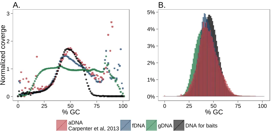
S5B). The higher number of nonduplicate mtDNA reads in capture 2 thus produced much deeper overall coverage of the mitochondrial genome (Figure S5C), despite the fact that the ratio of mtDNA to nuclear DNA mapped reads was compara-ble between the two captures (Figure S5D). Finally, the dis-tributions of read GC content for postcapture reads using our protocol, the DNA template for the RNA baits, and aDNA libraries were highly similar (Figure S6). This observation suggests that any GC bias relative to the genome appears during bait construction and/or sequencing, not during the hybridization step.
Postcapture fDNA-derived genotype data are consistent with individual identity and independently established pedigree relationships
To assess the accuracy of genotypes called from postcapture fDNA libraries, we compared genotype data from paired
blood-derived gDNA (without capture) and postcapture fDNA libraries for two individuals, LIT and HAP. Using genotypes for sites that were called with a genotype quality (GQ).20 in both the fDNA and gDNA data sets for either LIT or HAP, we found that the majority of the genotypes called in both data sets were concordant (86.5% of 312,739 sites for the LIT paired samples; 77% of 40,132 sites for the HAP paired sam-ples, for whom we had much lower coverage for the fecal-derived sample). As expected, the majority of the discordant sites occurred when the low-coverage fDNA sample was called as homozygous and the high-coverage gDNA sample was called as heterozygous (77.7% and 74.4% of discordant sites in LIT and HAP, respectively;Figure S7). Further, among all sites, the fDNA genotype captured at least one of the alleles from the gDNA genotype in 99.8% (LIT) and 99.6% (HAP) of cases (Figure S7). Thus, even when genotypes called in fDNA and gDNA samples from the same individual were discordant, they were almost always compatible.
Further, we found that genotypes called from the post-capture fDNA libraries were more similar to the genotypes called from their high-quality gDNA counterparts than they were to those from other postcapture fDNA libraries. Specif-ically, k0 values from lcMLkin (Lipatovet al. 2015), which estimate the probability that two samples share no alleles that are identical by descent, were much smaller for the LITfDNA–LITgDNA paired samples (0.487) and HAPfDNA–
HAPgDNApaired samples (0.243) than fork0 values
calcu-lated for the two blood-derived samples when compared to any other fDNA sample (k0 range LITfdnavs.other fDNA
sam-ples = 0.996–1.000;Z= 849.2,P,10220;k0 range HAP fDNA
vs.other fDNA samples = 0.786–0.999;Z= 10.6,P,10220;
Figure 4A).
For the 48 extended-pedigree individuals (Figure 1, in-cluding 8 Amboseli baboons with no known relatives in the pedigree), we then tested whether the estimated coefficient of relatedness values,r, fromlcMLkin(Lipatovet al.2015) in the postcapture data (range: 0–1, or 23the kinship coeffi -cient) were correlated with coefficient of relatedness values obtained from the independently constructed pedigree (based on known mother–offspring relationships and micro-satellite-based paternity assignments: see Methods). Using a filtered set of 127,654 single-nucleotide variants (see
Methods), we found a strong correlation between the two
measures (Pearson’sr= 0.73,P,10216; Figure 4B). This
correlation improved further if we imposed thresholds for the minimum number of sites genotyped in both individuals (“shared sites”) in a dyad (Figure S8). For example, if we removed all dyads with ,2000 shared sites (84 of 1128 dyads or 7.4%), the correlation between pedigree related-ness and genotype similarity reached Pearson’s r = 0.86 (P, 10216). Notably, for one individual we prepared and
sequenced capture libraries from two independently col-lected fecal samples (libraries AMB_018 and AMB_040). For these biological replicates, the pairwise relatedness value was 0.774, more than twice as high as for any other pair of relatives (range of estimates for parent–offspring and full-sib pairs typed at $2000 sites: 0.10–0.38). Thus, our methods readily distinguish replicate samples (which can be inadver-tently collected, especially in unhabituated populations) from those collected from distinct individuals, even close relatives.
Paternity inference using WHODAD
Current methods for assigning paternity [e.g., CERVUS (Marshallet al.1998; Kalinowskiet al.2007) and exclusion (Chakrabortyet al.1974)] assume genotype certainty, such that individuals are assigned a deterministic genotype at each locus (i.e., 0, 1, or 2 or a microsatellite repeat number; while a low level of measurement error due to sample mishandling can be modeled, this error rate is held constant across geno-type calls). This assumption is violated in low-coverage se-quencing data, in which genotypes are not known with certainty and this uncertainty varies across genotype calls.
However, the relativeprobabilitiesof each genotype can be estimated, given estimated population allele frequencies and sequencing coverage information. To conduct paternity in-ference and pedigree reconstruction in this context, we there-fore developed a novel approach to integrate information across low-coverage sites, implemented in the program WHODAD. Our method has two components. Thefirst com-ponent identifies a top candidate male and tests whether he is significantly more related to the offspring than any other candidate male, using aP-value criterion. The second com-ponent tests whether the dyadic similarity between the top candidate and offspring is consistent with a parent–offspring dyad, using posterior probabilities obtained from a mixture model (seeMethodsandFigure S9).
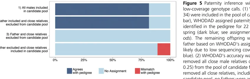
Using WHODAD, we assigned paternity to all father– off-spring pairs (n= 27) represented in the independently estab-lished extended pedigree in Figure 1. This approach is conservative because it departs from the usual practice offirst identifying a likely set of candidate fathers based on demo-graphic and prior pedigree information (the approach used in producing the pedigree in Figure 1). For 15 of the 27 off-spring, we produced genotype data from the known mother with our enrichment protocol. WHODAD identified the same father as shown in the pedigree in 12 of these 15 trios (80%); in the other 3 trios (20%), no candidate male satisfied WHODAD’s paternity assignment criteria (in all 3 of these cases, sequencing coverage was very low for either the pedigree-identified father or offspring: 0.04–0.173). For the remain-ing 12 offsprremain-ing, we did not generate genotype data usremain-ing our enrichment protocol for their mothers. To test all 27
Figure 2fDNA enrichment results. (A) Percentage of sequencing reads that mapped to the baboon genome and were not PCR duplicates (“Mapped,”dark blue), mapped and were PCR duplicates (“PCR Duplicate,”
blue), or did not map and likely represent environmen-tal or bacterial DNA in the case of fDNA/aDNA and unmappable fragments in the case of gDNA (“Other,”
father–offspring dyads together, we therefore reran WHODAD, excluding maternal genotype information. In this setting, WHODAD’s paternity assignments agreed with the pedigree data in 22 of 27 (81%) cases (Figure 5). Notably, when the pedigree-identified father was included in the data set, WHODAD never assigned paternity to a different male, whether or not maternal genotype data were available. Be-cause our method is highly robust to exclusion of maternal genotype data, we therefore performed all subsequent analy-ses assuming maternal genotype data werenot available, a scenario that may often occur in studies of natural populations. The presence of close relatives, such as full- or half-siblings, can influence the accuracy of paternity assignment if these close relatives are also included as candidate fathers (Thompson and Meagher 1987; Marshallet al.1998; Olsenet al.2001; Ford and Williamson 2010). Thus, to examine how the pres-ence of close male kin influenced the accuracy and confi -dence of WHODAD’s paternity assignments, we conducted three additional analyses. First, when all close male kin were removed from the candidate list of potential fathers
(r$0.25), but the father was retained, our method per-formed equivalently to the case when both father and close relatives were in the candidate pool. Second, when we re-moved all close male kinincludingthe father, none of the best candidate fathers from the conditional probability analysis (0%) were assigned as fathers based on WHODAD’s assign-ment criteria (Figure 5). Third, when we removed the father from the pool of candidate fathers, but included close male kin, 11% of the best remaining candidates (3 of 27 cases) were incorrectly assigned as fathers, based on comparison to the pedigree (Figure 5). All 3 of these false positives were close male relatives: in two cases WHODAD assigned the half-brother of the offspring as the likely father, and in one case WHODAD assigned the son of the offspring as the likely father. The best balance between maximizing the number of true positives while minimizing the number of false positives was achieved by combining both the P-value and mixture model criteria (see Methods). This approach outperformed either component used alone (Figure S10). For example, when all males were included in the candidate pool, the
Figure 3 Increased sequencing effort produces in-creased numbers of nonduplicate reads. Shown is the number of mapped reads plotted against the number of nonduplicate reads mapped [mean6 SD; plotted using the program “preseq” (Daley and Smith 2013)]. More complex libraries (i.e., those containing more nonduplicate fragments) have a slope closer to 1 (as in the case of the gDNA libraries), while less complex libraries have a shal-lower slope and asymptote at a smaller value. The main plot shows thefirst 10 million mapped reads for each sample. The inset shows the same plot for thefirst 1 million mapped reads.
combined approach resulted in an 81% true positive rate and a 0% false positive rate, while using just thek0 values in a mixture model resulted in the same true positive rate (81%), but an additional 11% false positive rate (Figure S10).
Discussion
Our capture-based method strongly enriches the proportion of host DNA in low-quality DNA extracted from feces (fDNA). Our method is thefirst use of genome-wide enrichment-based capture methods (Carpenter et al. 2013; Enk et al. 2014; Ávila-Arcoset al.2015) for noninvasively collected samples, which represent a major resource for behavioral, conserva-tion, and evolutionary genetic studies in natural populations. Importantly, our protocol increases efficiency and lowers cost by reducing the input requirements (,1mg) and number of PCR cycles relative to previous methods (Perryet al.2010) and, in ourfinal protocol, achieves up to 40-fold enrichment of postcapture endogenous DNA relative to precapture levels. We also show, for thefirst time since Perryet al.(2010), that capture libraries from low-quality samples produce geno-type data that are highly concordant with genogeno-type data derived from high-quality, noncaptured samples from the same individuals.
We anticipate that data generated through this protocol could be leveraged for a wide variety of applications. To illustrate this point for paternity analysis, we present an accompanying method, WHODAD, that produces results in near-perfect concordance with an independently constructed pedigree, using low-coverage data generated with our enrich-ment protocol. By incorporating prior information about ped-igree links or other demographic and behavioral data, or by sequencing very low-coverage samples to additional depth (similar to typing more markers in conventional microsatellite analysis), its performance would be improved even further. For instance, in reconstructing pedigree links in the Amboseli population, we generally include only plausible candidates (e.g., we exclude males who were immature or not yet born at the offspring’s conception), not all males with genotype data, as we did here.
Together, these results provide valuable, accessible wet laboratory and computational tools for moving studies of difficult-to-sample natural populations forward into the ge-nomics era. Importantly, our methods can be generalized to produce low-complexity DNA-depleted RNA baits for any species in which at least one high-quality DNA sample is available [or potentially a closely related species (Enket al.
2014)]. Further, our results show that WHODAD is highly accurate for pedigree reconstruction even when the reference genome is not a high-quality chromosomal assembly (here, we used 33,120 contigs from Pcyn1.0) or, based on explor-atory analyses, even from the same species. Specifically, when mapping to the reference genome for the rhesus ma-caque [MacaM(Ziminet al.2014)] instead of baboon, which diverged from baboons 6–8 MYA (Steiper and Young 2006), WHODAD produced similarly accurate paternity assignments (21 of 27 fathers were correctly assigned using our recom-mended statistical thresholds compared to 22 of 27 when mapping toPcyn1.0; there were no false positive assignments in either case).
Costs of performing the protocol
At the time of publication, using the same reagents as we used here and sourced from the same locations, the costs of gen-erating these data are $60 per sample (excluding se-quencing costs). Because our method does not require the commercial synthesis of targeted capture probes, the major-ity of the costs are accounted for by the streptavidin-coated Dynalbeads ($11 per preparation), RNA baits ($5 per sam-ple) and high-sensitivity Bioanalyzer chips for quality control ($9 per sample). Replacing Ampure XP beads with home-made SPRI beads would reduce the per-sample costs consid-erably, as would pooling adapter-ligated fDNA samples prior to hybridization (instead of posthybridization, as reported here). For a multiplexed pool of 10 samples, we estimate that using these two strategies would result in a per-sample cost of $29. Indeed, we have verified that multiplexing samples prior to hybridization does not result in loss of capture effi -ciency and actually resulted in improved yield of mapped, non-PCR duplicate reads (61% of reads; mean of 117-fold
enrichment, range = 54.8–257.2-fold; Figure S11A), al-though it did result in more uneven coverage of samples sequenced within a pool (Figure S11B) and raises the possi-bility of barcode swapping [which can be managed using dual barcoding approaches (Kircher et al. 2012)]. Multiplexing also has the advantage of reducing the amounts of input DNA per sample and the number of PCR cycles required for the initial library preparation step. We are currently pursuing improvements to the protocol along these lines.
Based on achieving 40% non-PCR duplicate, mapped reads after capture (the mean result for capture 2 samples), we estimate that the sequencing costs of a 13genome for baboon (2.9 Gb) would be$200 (based on paired-end, 125-bp sequencing at $2000 per lane and exclusion of PCR dupli-cates). This cost per sample is approximately twice the cost of genotyping 14 microsatellites from the same fDNA sample— the previous strategy for the main study population, the Amboseli baboons (Van Hornet al.2008)—but provides sub-stantially more genetic information. These estimates will drop farther as the cost of high-throughput sequencing con-tinues to fall, making application of our approach to whole populations increasingly feasible. Ourfinding that useful se-quencing reads do not asymptote with deeper sese-quencing (Figure 3) also suggests the feasibility of producing a high-quality, high-coverage genome from such samples if one were to sequence more deeply. This approach would alleviate cases in which both alleles at a truly heterozygous site were not observed due to low sequencing depth (for example, with 13 coverage, only one of the two alleles can possibly be ob-served). Notably, however, it would notfix“allelic dropout” problems in which an allele was not represented in the pool of sequenceable fragments (Pompanonet al.2005). Analo-gous to the solution in noninvasive microsatellite typing, multiple, independent PCR reactions could be used to solve this problem.
Finally, to make the current protocol as cost effective as possible, we recommend that researchers use qPCR to choose DNA samples with the highest proportion of host DNA pos-sible—the strongest predictor of the fold-change enrichment in endogenous DNA postcapturevs.precapture (Figure 2D).
Assigning paternity using WHODAD
The lack of available tools for working with low-coverage genomic data—realistically, one of the most likely data types to be produced for studies of natural populations—represents a major barrier to moving from low-throughput marker geno-typing to genome-scale analyses. The pedigree structure of a study population is fundamental to understanding its genetic structure and social organization. However, current methods for pedigree reconstruction are unable to cope with high lev-els of genotype uncertainty. The approach we have imple-mented in WHODAD takes this uncertainty into account, suggesting one simple application for the wet laboratory methods presented here. Indeed, our method performed well when compared to an independently constructed extended pedigree, with its major challenges—differentiating between
close relatives in a candidate pool—comparable to those re-ported for existing software (Marshallet al.1998; Olsenet al.
2001; Kalinowskiet al. 2007; Ford and Williamson 2010). Importantly, while analyses of pedigree structure using pre-viously available methods are greatly aided by prior knowl-edge of mother–offspring relationships (Kalinowski et al.
2007), maternal links do not appear to be necessary for WHODAD analyses, which perform well even when no ma-ternal information is available (Figure 5,Figure S9). Conclusions
High-throughput sequencing approaches solve one problem of working with low-quality, noninvasive samples: the sheared nature of the original samples. Capture approaches have demonstrated great promise for solving the second major problem—large proportions of nonendogenous DNA—since the results published by Perryet al.(2010). Our results help to fulfill this promise by providing methods to perform cost-effective sequence capture from noninvasive samples on a genome-wide scale, coupled with analytical methods to deal with the resulting data (we note that our protocols could also be explored for broader application to aDNA samples). For questions in which investigators are specifically interested in variants ina priori-defined subsets of the genome [e.g., the exome (Vallender 2011; Georgeet al.2011)], targeted cap-ture with synthesized baits may still be the best option. How-ever, for the many types of analyses that use genome-scale data [e.g., local ancestry analysis, genome-wide scans for selection, and reconstruction of population demographic his-tory (Sabetiet al. 2002; Huanget al.2007; Liet al.2007; Sankararaman and Sridhar 2008; Priceet al.2009; Durand
et al.2011; Li and Durbin 2011; Yanget al.2011; Maet al.
2014)], our approach will be more useful, especially as the costs of high-throughput sequencing continue to fall.
Here, we focused specifically on DNA obtained from fecal samples, which are one of the most commonly collected types of noninvasive samples: they contain information not only about host genetics, but also about endocrinological param-eters (Palme 2005), gut microbiota (Leyet al.2008), parasite burdens (Gillespie 2006), and gene expression levels (Knight
et al. 2014). The sample banks already available for many natural populations thus open the door to population and evolutionary genomic studies in species in which such anal-yses were previously impossible. As the costs of data gener-ation continue to fall, and the limiting factor for many studies becomes high-quality phenotypic data, we envision that such studies will rapidly move far beyond the simple analyses of paternity and pedigree structure reported here.
Methods
Bait generation
Similar to Carpenter et al. (2013), we use a cost-effective
collected from an olive baboon (P. anubis) that was unrelated to any of the individuals in the samples we wished to enrich. To generate baits, we sheared 5mg of purified DNA to a mean fragment size of 150 bp and then end repaired and A-tailed the fragments, using the KAPA DNA Library Preparation Kit for Illumina Sequencing. We purified the resulting reaction, using a 1.83ratio of AMPure beads to sample volume.
We annealed custom adapters to the A-tailed library by incubating the following reagents for 15 min at 20°: 10ml 53 ligation buffer (KAPA Biosystems), 5 ml DNA Ligase (KAPA Biosystems), 1ml 25mM custom adapter,#34ml of A-tailed DNA, and H2O up to 50ml total volume. The custom
adapt-ers we used (EcoOT7dTV, Fwd 59-GGAAGGAAGGAAGA GATAATACGACTCACTATAGGGCCTGGT; EcoOT7dTV, Rev
59-/5Phos/CCAGGCCCTATAGTGAGTCGTATTATCTCTTCC
TTCCTTCC) differ from those used in other protocols (Carpenter et al. 2013; Enk et al. 2014; Ávila-Arcoset al.
2015). Specifically, they contained (1) a T7 RNA polymerase recognition site, (2)flanking sequence that improves T7 tran-scription efficiency (Mollet al.2004), and (3) an EcoO109I restriction enzyme cut site that allowed us to later cleave off the adapter sequence from T7 amplified RNAs (rather than blocking it, as in Carpenteret al.2013).
We then digested the purified, adapter-ligated DNA with DSN (Axxora). DSN is a Kamchatka crab-derived enzyme that specifically degrades double-stranded DNA but not single-stranded DNA, allowing us to take advantage of DNA reasso-ciation kinetics to reduce the representation of repetitive regions in the bait set (Figure S2; Shaginaet al.2010). We performed DSN digestion in 15 2-ml aliquots, each mixed with 1 ml 43 hybridization buffer [200 mM HEPES (pH 7.5), 2 M NaCl, 0.8 mM EDTA] and 1ml human Cot-1 DNA (1 mg/ml). We denatured the DNA by heating to 98° for 3 min; held the reaction at 68° for 4 hr; and then added 4ml H2O, 1 ml 103DSN buffer, and 1 ml DSN (1 unit/ml)
to the reaction. After 20 min of digestion, we stopped the reaction by adding 5ml 23DSN Stop Solution (10 mM EDTA) and purified it with 2.43AMPure beads.
Next, we used Klenow DNA polymerase to blunt end the nondigested DNA, size selected for 200- to 300-bp fragments on a 2% agarose gel, and purified the size-selected fraction using the Zymoclean Gel DNA Recovery Kit (Zymo Research). After purification the aliquots were PCR amplified for 16 cycles, using 25ml 23HiFi Hot Start ReadyMix (KAPA Bio-systems) and 1 ml each of 25 mΜ primers EcoOT7_PCR1 (59-GGAAGGAAGGAAGAGATAATACGACTCACT) and EcoOT7_ PCR2 (59-TACGACTCACTATAGGGCCTGGT). Following amplifi -cation the bait DNA libraries were purified using 1.83AMPure beads and the resulting product was visualized on a Bioanalyzer DNA 1000 chip (Agilent Technologies).
Finally, wein vitro transcribed the DNA libraries to con-struct biotin-tagged RNA baits, using the MEGA Shortscript Kit (Life Technologies) and Biotin-UTP (Illumina). Briefly, 125–150 nM of DNA baits were incubated at 37°for 4 hr in the following reaction: 2ml T7 103reaction buffer; 2ml each of T7 ATP, GTP, CTP, and UTP solutions (75 mM); 1ml
Biotin-UTP (50 mM); 2ml T7 enzyme mix; and water to 20ml total volume. We then digested the DNA template by adding 1ml TURBO DNase (Life Technologies) to the reaction and incu-bating it at 37°for 15 min. We purified the resulting reaction with the MEGAClear Transcription Clean-Up Kit (Life Tech-nologies) and eluted it in afinal volume of 70ml. To cleave off the adapter sequence, we digested the RNA baits with the
EcoO1091 enzyme (NEB). Finally, the baits were again puri-fied with the MEGAclear Clean-Up Kit, eluted in 70ml, and quantified on a Bioanalyzer RNA 6000, Eukaryote Total RNA chip (Agilent Technologies).
Samples, DNA extraction, and qPCR quantification
Baboon samples from Amboseli (the main study population) or West Africa (8 unhabituated Guinea baboons) were col-lected, stored, and extracted as detailed inTable S2. For LIT and HAP, gDNA was extracted from blood samples, using the QIAGEN (Valencia, CA) Maxi Kit. The majority of the sam-pled Amboseli individuals (48 of 54) were either members of a single extended pedigree or unrelated males living in the same study population (Figure 1). We assessed the proportion of endogenous DNA in each fDNA sample, using qPCR against thec-mycgene, as described in Morinet al.(2001).
Library preparation
All samples were fragmented to the desired size (200 or 400 bp; seeTable S1), using a Bioruptor instrument (Diagenode). Illumina sequencing libraries were then generated from the fragmented DNA, using either the KAPA DNA library kits for Illumina (capture 1) or the NEBNext DNA Ultra library kit (capture 2; seeTable S1). Libraries were amplified for 6 PCR cycles prior to capture-based enrichment. Sample-specific tails of library preparation and sequencing results are de-scribed in Table S1. Note that we changed several steps between capture 1 and capture 2 based on interim improve-ments in the protocol (also detailed inTable S1). Because the methods used in capture 2 were ultimately more effective, the updated capture 2 protocol is described in theMethods
section except where explicitly noted.
Capture-based enrichment
After incubation, we purified the enriched fDNA sample, using 50ml Dynal MyOne Streptavidin T1 beads (Invitrogen, Carlsbad, CA). To do so, the beads were washed a total of three times with 200ml binding buffer [1 M NaCl, 10 mM Tris-HCl (pH 7.5), 1 mM EDTA] and resuspended in 200ml binding buffer. Next, the entire fDNA/RNA hybridization mix was added to the 200-ml Dynal MyOne Streptavidin T1 bead and binding buffer slurry. We incubated this mixture at room temperature for 30 min on an Eppendorf Thermomixer at 700 rpm. The mixture was placed on a magnetic rack, the supernatant was discarded, and the beads were washed once with 500ml low-stringency wash buffer (13SSC, 0.1% SDS) followed by a 15-min incubation at room temperature. The beads were then washed three times with 500 ml high-stringency wash buffer (0.13SSC, 0.1% SDS) with a 10-min room temperature incubation between each wash. After the final wash, the enriched fDNA fraction was eluted from the beads with 50ml elution buffer (0.1 M NaOH), transferred to a new tube containing 70ml“neutralization buffer”(1 M Tris-HCl, pH 7.5), purified with 1.83AMPure beads, and eluted in a 30-ml volume. Afinal PCR was carried out in a 50-ml reaction volume, using 23ml of the posthybridization fDNA and either (1) 25ml 23KAPA High Fidelity master mix and 2 ml TruSeq universal primer (capture 1) or (2) 25ml 23 NEB-Next High Fidelity PCR master mix, 1 ml universal PCR primer, and 1ml NEB indexing primer (capture 2). After 12 PCR cycles thefinal reaction was purified with 13AMPure beads, eluted in 20mL H2O, and visualized on a Bioanalyzer
High Sensitivity DNA chip.
Sequencing and alignment
All high-throughput sequence generation was conducted on the Illumina HiSeq platform (see Table S1 for sequencing details). The resulting sequencing reads were mapped to a de novo assembly of the P. cynocephalus genome (Wall
et al. 2016) (alignment available athttps://abrp-genomics. biology.duke.edu/index.php?title=Other-downloads/Pcyn1.0), using the default settings of thebwa memalignment algo-rithm v0.7.4-r385 (Li 2013). Reads that mapped to scaffold 10204 of Pcyn1 were assigned to mitochondrial DNA due to scaffold 10204’s similarity (97% sequence similarity) to a publishedP. anubismitochondrial genome (NCBI GenBank accession no. KC757406.1). Duplicate reads were marked and discarded in subsequent analyses, using the“ MarkDupli-cates” function in PicardTools (http://picard.sourceforge. net). To facilitate comparison across samples of differing cov-erage, and because coverage of the gDNA samples was much higher (303) than for the fDNA samples for LIT and HAP (1.4 and 0.27, respectively), we downsampled the gDNA li-braries to 0.733coverage (the median coverage of samples in capture 2), using“DownsampleSam”in PicardTools.
Comparison of sequencing data sets
In several analyses, we compared our capture-based enrich-ment results to two independent data sets: (i) a previously published capture-based enrichment of aDNA samples [NCBI
SRA accession no. SRP042225 (Carpenteret al.2013)] and (ii) shotgun sequencing from six capture 1 fDNA samples prior to hybridization (“precapture”; Table S1). The aDNA samples were aligned to the human genome (hg38) and the precapture fDNA samples were mapped to the de novo Pcyn1.0genome assembly.
Library complexity, distribution of reads, and GC content
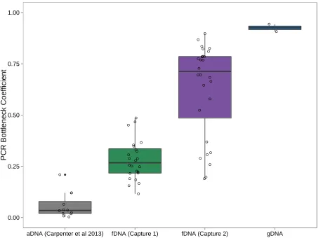
We calculated the complexity of each library, using two methods. First, we used the ENCODE Project’s PCR bottle-neck coefficient (PBC), which calculates the percentage of nonduplicate mapped reads from the total number of mapped reads (Kharchenko et al. 2008; Landt et al. 2012).The PBC ranges from 0 to 1, where more complex libraries have higher numbers. Second, we used the function“c_curve”from the pro-grampreseq(v1.0.2) to plot the number of nonduplicate frag-ments mapped vs. the number of total mapped fragments (Daley and Smith 2013). More complex libraries (i.e., those with fewer duplicate fragments) have a c_curve slope closer to 1, meaning that increasing sequencing depth continues to provide novel information. Less complex libraries have a shal-lower slope and asymptote at smaller values. Finally, we evalu-ated the GC bias for each sequencing library, using Picard Tools’ “CollectGCBiasMetrics”(http://picard.sourceforge.net).
Sample attributes influencing capture efficiency
To determine the sample attributes that predicted the success of our capture protocol, we first modeled the relationship between the proportion of nonduplicate reads that mapped to the baboon genome after capture (our primary measure of protocol success) and (i) the percentage of endogenous ba-boon DNA in the precapture samples, (ii) the amount of fDNA library (nanograms) that went into the capture, and (iii) whether the sample was captured using our initial protocol or the second version of the protocol (i.e., in capture 1 or capture 2). Second, we investigated the relationship between the same three variables and a secondary measure of protocol success, the fold-change enrichment of baboon DNA in the sample precapture vs. postcapture. Precapture concentra-tions of endogenous DNA in fDNA samples were measured as the concentration of baboon DNA estimated using qPCR, relative to the concentration of total DNA estimated using the Qubit High Sensitivity fluorometer (Life Technologies). To ensure that our qPCR-based measures were well calibrated, we confirmed the relationship between qPCR-based esti-mates and precapture sequence-based estiesti-mates of endoge-nous DNA in six samples for which both values were available (R2= 0.92;Figure S13). All statistical analyses were carried
out in R (R Development Core Team 2015).
Variant calling
We used two different approaches to call variants and geno-types in our sample: SAMTOOLS (Li et al. 2009; Li 2011) and the Genome Analysis Toolkit (GATK) (McKenna et al.
downstream analyses, we retained only variants that were identified by both methods, a strategy that produces a higher ratio of true positives to false positives than variants identified by a single method alone (O’Rawe et al. 2013). Duplicate-marked alignments were used as input for both methods. SAMTOOLS multisample variant calling was carried out using
mpileup and bcftools, with a maximum allowed read depth (-D) of 100. GATK variant calling was carried out using Hap-lotypeCaller following the GATK v3.0 Best Practices for variant calling from DNA-seq. To minimize potential batch effects in-troduced by the two capture efforts, we used the following strategy. First, we called genotypes using reads from each capture independently. Second, we recalled genotypes us-ing reads from both captures together. Third, we extracted the union set of variants called in steps 1 and 2 for down-stream analysis.
Because no reference set of genetic variants is currently publicly available for baboons, we used a bootstrapping pro-cedure for base quality score recalibration. Briefly, we per-formed an initial round of variant calling on read alignments without quality score recalibration. From this variant call set, we extracted a set of high-confidence variants that passed the following hardfilters: quality score$100; QD,2.0; MQ, 35.0; FS . 60.0; HaplotypeScore .13.0; MQRankSum , 212.5; and ReadPosRankSum, 28.0 (as described in Tung
et al.2015). We then recalibrated the base quality scores for each alignment, using this high-confidence set as the data-base of“known variants,”and repeated the same variant-calling andfiltering procedure for three additional rounds. Finally, we identified the intersection set between the var-iants called from GATK and SAMTOOLS, respectively, us-ing the bcftoolsfunctionisec(Liet al.2009). To produce ourfinal call set, we removed all sites that were genotyped in only one of the capture efforts, had a minor allele fre-quency of ,0.05, or were within 10 kb of one another, usingvcftools(Daneceket al.2011). For comparisons be-tween the paired fDNA and gDNA samples, we used the above variant-calling pipeline to jointly genotype all sam-ples sequenced in the study.
Estimating the coefficient of relatedness
To produce an estimate of relatedness between samples in our pedigree and to test for concordance between fecal and blood-derived samples for the same individuals, we used the program
lcMLkin(Lipatovet al.2015).lcMLkinuses the genotype likeli-hoods generated by GATK for each genotype call to calculate two measures: (i) k0, the probability that two individuals share no alleles that are identical by descent, and (ii) r, the coefficient of relatedness (Lipatovet al.2015) (i.e., twice the kinship coefficient). Several other methods have been developed (Manichaikulet al.2010; Yanget al.2010) to estimate related-ness from thousands of SNPs, butlcMLkinyielded the best match to pedigree-based estimates in our data set (Figure S14).
We also compared genotype calls for the matched fecal and blood-derived samples, using GATK’s GenotypeConcordance function (DePristo et al.2011). This tool allowed us to
de-termine concordance rates between data sets for different classes of variants (e.g., 0, 1, or 2).
WHODAD: paternity inference and pedigree reconstruction
Our paternity prediction model is based on a naive Bayes classifier that takes advantage of the rules of Mendelian segregation within pedigrees. Using data from all sites geno-typed in a potential father–mother–offspring trio or, when the mother is not genotyped, all sites genotyped in a potential father–offspring dyad, it estimates the posterior probability that a potential candidate is the true father of a given offspring.
Our approach can be broken into three steps (Figure S9). First, we estimate, for each candidate male, the conditional probability that he is the true father of a given offspring, given the genotype data for the candidate, offspring, and mother, if known (below we show the case in which genotype informa-tion is available for the mother, but the model is similar when maternal genotype information is missing). Second, we as-sign aP-value for the top candidate male from thefirst step, for the null hypothesis that he isnotmore related to the focal offspring than the other candidates tested. Third, we calcu-late the probability that the genotype data for the top candi-date and offspring are consistent with a true parent–offspring relationship, using a mixture model. Steps 2 and 3 perform subtly different functions in our analysis: step 2 tests that the top candidate is significantly more related to the offspring than any other candidate, whereas step 3 tests that the dyadic similarity between the candidate and the offspring looks as expected for parent–offspring dyads. We have found that combining both approaches is key to detecting true positive fathers while minimizing false positive calls that can occur when true fathers are not in the pool of genotyped candidates (Figure S10).
Step 1: estimating conditional probabilities for each trio: For a given offspring or mother–offspring dyad, our goal is to infer the true genetic father from a pool ofncandidates. For theith candidate, we use data for theLivariants for which we have genotype information for the known mother–offspring dyad and for the candidate father. Assuming the true father is present in the candidate pool (i.e., he has been genotyped), the probability that theith potential candidate is the father is
PðFijM;OÞ ¼PðFi;M;OÞ
, Xn
k¼1
PðFk;M;OÞ
!
; (1a)
PðFijM;OÞ PðFi;M;OÞ1=Li
, Xn
k¼1
PðFk;M;OÞ1=Lk
!
:
(1b)
Each joint probability can be calculated in turn as
PðFi;M;OÞ ¼
X
f;m;o
PðFi;M;O;f;m;oÞ
¼ X
f;m;o
YLi
j¼1
PðFi;M;O;fij;mj;ojÞ; (2)
wheremj,fij, andojrepresent the genotype data for thejth variant of the mother, the candidate father, and the offspring, respectively. Genotypes take values in {0, 1, 2} (i.e., the num-ber of copies of the reference allele at each individual–site combination). Importantly, although Equation 2 unrealisti-cally assumes independence across loci, this assumption does not change the relative order of trio joint probabilities.
The probabilityPðFi;M;O;fij;mj;ojÞfor each locus can be further decomposed as
PFi;M;O;fij;mj;oj
}Pojjmj;fij
PfijjFi
PmjjMPojjO Poj
;
(3)
where we take genotype uncertainty into account by using GATK’s genotype probabilities to calculate the conditional genotype probabilities forPðfijjFiÞ;PðmjjMÞ;andPðojjOÞover all possible genotype values at each site–individual combina-tion (i.e., the probabilities that each genotype is 0, 1, or 2, which sum to 1). We also ignore the scaling constant
PðFiÞPðMÞPðOÞbecause it cancels out in the numerator and denominator of (1). The marginal probability of the off-spring’s genotype,P(oj), is calculated from the minor allele frequency of the variant in the population. Finally, the condi-tional probabilityPðojjmj;fijÞis based on the rules of Mende-lian transmission (e.g., Marshallet al.1998). Due to genotype uncertainty in low-coverage data, the values ofPðFijM;OÞ are small. However, the highest value is usually assigned to the most likely father (based on comparison to the pedi-gree; seeResults) and we can directly assess the strength of the relative evidence for the top candidatevs.other candi-dates in step 2 by calibrating these values against per-muted data.
Step 2: calculating resampling-based P-values:To compute
P-values for each paternity assignment, candidates are ranked based on their conditional probability PðFijM;OÞ of being the true father. The log ratio of conditional probabilities between the highest-probability father and the second best candidate is the test statistic
v¼log PðFbestjM;OÞ
PðFsecondjM;OÞ !
: (4)
To assess significance forv, we then simulate genotype data for a set of n unrelated candidate fathers based on allele frequency information for each locus in the analysis and se-quence coverage information for the real candidates, at each of the loci for which they were genotyped in the true data set. Specifically, for each locus-simulated unrelated candidate combination, fij, where i indexes a (real) candidate male and j indexes the locus, we simulate a vector of genotype probabilities for the candidate father, ðfij0;fij1;fij2Þ; which
sum to 1. The number of probability vectors simulated for each candidate is based on the number and identity of the loci observed in the real data. For example, if the top candi-date in the real data were evaluated based on 10,000 sites, we would simulate an unrelated male with genotype vector probabilities simulated for each of those 10,000 sites; if the second-best candidate was evaluated at 9000 sites, we would simulate an unrelated male with genotype vector probabili-ties simulated for each of those 9000 sites, and so on. The variant sets for different simulated candidates need not be identical and are in fact highly unlikely to be so in practice.
To simulate each vector, we draw values from a Dirichlet distribution (i.e., a distribution on probability vectors that sum to one). In principle, the Dirichlet distribution for each biallelic site could be parameterized by the genotype frequen-cies for each of the three potential genotype values, Dirðpj0;pj1;pj2Þ; with genotype frequencies equal to the
Hardy–Weinberg expected values based on the allele fre-quency of the reference allele [i.e.,p2, 2p(12p), (12p)2,
withpestimated from the data]. However, the low coverage in our data introduces additional noise into this sampling problem, so we instead draw values from the following Dirichlet distribution,
ðfij0;fij1;fij2Þ Dirðkcijðpj0;pj1;pj2ÞÞ; (5)
wherecijis the read depth (coverage) for the site in (true) candidate fatheri, andkis a concentration parameter com-mon to all sites and candidate fathers, estimated from the real data using the method of moments. kcan be thought of as a scaling factor for the effect of coverage on variance in ðfij0;fij1;fij2Þ:To make the simulations as realistic as possible,
all parameters are estimated from the real data as
pjl¼EðfijlÞ; (6)
where the expectation is based on the allele frequencies for the reference allele estimated across all individuals, for each locus
jand genotypelcombination, and
k¼ EðfijlÞ2E
fijl2 Ecijfijl2
2E2ðc ijfijlÞ
; (7)
observed average values from the data, which approximate the expected value.
After simulating genotype data for each candidate male as if he were unrelated to the focal offspring, we can obtain a new value ofv(Equation 4) from the simulated data. By repeating this procedure s times, we can compute a P-value for the hypothesis that the best candidate in the true data is no more related to the focal offspring than any other candidate in the data set. ThisP-value is equal to the proportion of times the simulated test statistics exceed the observed test statistic. It intuitively corresponds to the probability of seeing a gap as large as the true gap between the conditional probabilities for the best and second-best candidates, if all candidates were in fact unrelated (or equally related) to the focal offspring.
Step 3: estimating the posterior probability of paternity: WHODAD’s inference method, like other paternity inference methods [e.g., CERVUS (Marshall et al. 1998; Kalinowski
et al.2007)], can falsely assign paternity to a close relative if the true father is not included in the pool of potential fathers. Such false positives arise because these methods do not actually test the hypothesis that the assigned father is the true father, but rather whether the assigned father is signifi -cantly more closely related to the focal offspring than other candidates in the pool. A more direct method would be to test the probability of observing the data for a father–offspring dyad (or father–mother–offspring trio) under thealternative
hypothesis that the assigned father is the true father. Test-ing the alternative hypothesis is nontrivial with low-coverage data and by itself can also yield incorrect inferences ( Fig-ure S10). However, in combination with the resampling-based P-values described above, it can improve paternity assignments.
To estimate the probability of the data given the best candidate–offspring dyad, we take advantage of the fact that dyadic measures of genotype similarity or relatedness or other estimates of identity-by-descent should differ for true parent–offspring pairs compared to all other dyads (except for full sibs). By utilizing the many dyadic values in a data set of mothers, offspring, and candidate fathers, we should therefore be able to distinguish father–offspring dyads from dyads involving other relatives or unrelated pairs. Notably, this method allows us to use dyadic values for mother– off-spring pairs to maximum effect.
We use a normal mixture clustering approach and thek0 value from the R packagelcMLkin, where lowk0 values pre-dict a low probability of sharing 0 alleles. We denoteybas the
vector of logit-transformed k0 measurements for the best candidate–offspring dyads for all tested father–offspring dyads; y1 as the vector of logit (k0) measurements for all
known mother–offspring dyads, if any are present (y1 can
be an empty vector if no mother–offspring dyads were sam-pled); andy0as the vector of logit (k0) measurements for all
other dyads. Thus,y0captures the distribution of logit (k0)
values for non-parent–offspring dyads;y1captures the
distri-bution of logit (k0) values for known parent–offspring dyads;
andybcontains a mixture of logit (k0) values for both true
parent–offspring dyads and non-parent–offspring dyads. Wefirst work only withy0and use a mixture model
ap-proach to assign the logit (k0) value for each dyadiinto one ofKcomponent normal distributions (fitted using the mix-toolsfunction in R, with a default value ofK= 5; note that our analyses are robust to reasonable choices ofK, seeFile S1). Components with lower mean values fork0 can be thought of as capturing the distribution of logit (k0) values for highly related dyads (e.g., half-siblings), whereas components with high mean values capture distantly related or unrelated dyads (if relatedness coefficients were used instead of k0, this direction would be reversed: low values would corre-spond to distantly related dyads instead). For y1, all dyads
are from the same relatedness category (mother–offspring), so logit (k0) values iny1can be modeled by a single
distri-bution parameterized by a mean and a variance. Finally, for
yb, values of logit (k0) can be assumed to be drawn either
from the distribution on y1or from one of the distributions
(likely one with a low mean value) in the mixture model fory0,
ybi pN
m;s2þ ð 12pÞN
mi;s2i
; (8)
where for theith individual inyb,miands2i are the mean and variance for one of the distributions in the mixture model of
y0;mands2are the mean and variance for the distribution on
y1; andpis the probability that a value inybbelongs to the
parent–offspring distribution or one of the distributionsfitted in the mixture model for other dyads. To infer these param-eters, for each dyad inyb, we assignmi;s2i to the mean and variance of the mostly likely normal component by evaluat-ing the likelihood under allKcomponents. We then combine
y1andybto jointly inferp;m;s2 in Equation 8.
Finally, we introduce a latent indicator variablezbifor each dyad to indicate whether theith dyad inybis a true father–
offspring dyad. The probability of being a true father– off-spring dyad, orP(zbi= 1), becomes thefinal statistic used to assess our paternity assignments. To inferP(zbi= 1), we use an expectation-maximization algorithm (seeFile S1for detailed information about the EM steps). WHODAD con-siders a male as the likely true father of a focal offspring if he was (i) the candidate with the highest conditional proba-bility of paternity, (ii) assigned aP-value from our simulations ,0.05, and (iii)P(zbi= 1).0.9.
Testing the accuracy of paternity assignment using WHODAD
We assigned paternity using the methods detailed above for all previously identified father–offspring pairs (n= 27) in the Amboseli pedigree (Figure 1). This pedigree was constructed using a combination of observational life history data on female pregnancies and infant care (to infer maternal– offspring dyads), demographic data to identify possible can-didate fathers, and microsatellite genotyping data analyzed in the program CERVUS (with confidence.95%; see Alberts
Our data set contained maternal genotype information derived from the fecal enrichment protocol for 15 of these individuals (56%). Wefirst used WHODAD to assign paternity for these 15 offspring while incorporating the genotype data from their mothers. To assess the accuracy of WHODAD in the absence of maternal genotype data, we then repeated the paternity analysis for the same 15 offspring without including the mother’s genotype. For this analysis, we were also able to include the 12 additional offspring for whom we did not have genotype data from the mother, but had genotype data from the known father (n= 27).
To examine how the presence of close male kin influenced the accuracy and confidence of WHODAD’s paternity assign-ments, we conducted three additional analyses. First, to as-sess the accuracy of WHODAD when the pedigree-assigned father is the only close male relative present, we removed all close relatives of the offspring except the father (r$0.25,
e.g., grandfathers and half-sibling or full-sibling brothers) from the pool of potential fathers. Second, to test whether WHODAD assigned a father with high confidence even when no close relatives were present, we removed all close male relatives, including the pedigree-assigned father, from the pool of candidate males. Third, to assess the risk of confi -dently (but erroneously) assigning a close male relative as the likely father when the pedigree-assigned father was not genotyped, we removed the father from the pool of poten-tial fathers. For all WHODAD analyses we report assignment accuracy based on whether the father was identified by WHODAD with aP-value,0.05 and aP(zbi= 1).0.90. Offspring were not assigned a father (“no assignment”) when the best candidate male was identified with aP-value.0.05 or aP(zbi= 1),0.90.
Data availability
All sequencing data sets reported in this article have been deposited in the NCBI Short Read Archive (SRA), accession no. SRP064514. The authors state that all data necessary for confirming the conclusions presented in the article are rep-resented fully within the article.
Acknowledgments
We thank the Kenya Wildlife Service, the Institute of Primate Research, National Museums of Kenya, the National Council for Science and Technology, members of the Amboseli–Longido pastoralist communities, Tortilis Camp, and Ker & Downey Safaris for their assistance in Kenya. We also thank Jeanne Altmann and Elizabeth Archie for their generous support and access to the Amboseli Baboon Research Project data set and samples; Raphael Mututua, Serah Sayialel, Kinyua Warutere, Mercy Akinyi, Tim Wango, and Vivian Oudu for invaluable assistance with the Amboseli baboon sample collection; Emily McLean for assistance in identifying samples from the extended pedigree; and Tauras Vilgalys for assistance in drawing the pedigree. For access to the Guinea baboon samples, we thank Julia Fischer, Dietmar
Zinner and José Carlos Brito; the Wild Chimpanzee Founda-tion for logistical support in Guinea; and the Ministère de l’Environnement et de la Protection de la Nature and the Direction des Parcs Nationaux in Senegal; the Opération du Parc National de la Boucle du Baoulé and the Ministère de l’Environnement et de l’Assainissement in Mali; the Office Guinéen de la Diversité Biologique et des Aires Protégées and the Ministère de L’Environnement, des Eaux et Forêts in Guinea; and the Ministère Délégue auprès du Premier Ministre, Chargé de l’Environnement et du Développement Durable in Mauritania. Finally, we thank P. J. Perry, Luis Barreiro, Greg Crawford, Tim Reddy, members of the Alberts and Tung laboratories, and two anonymous reviewers for their feedback on earlier versions of this work. This work was supported by National Science Foundation grants DEB-1405308 (to J.T.) and SMA-1306134 (to J.T. and N.S.-M.). G.H.K. was supported by the German Academic Exchange Service [Deutscher Akademischer Austauschdienst (DAAD)], the Christiane-Nüsslein-Volhard Foundation, The Leakey Foun-dation, and the German Primate Center. X.Z. was supported by a grant from the Foundation for the National Institutes of Health through the Accelerating Medicines Partnership BOEH15AMP. The authors declare no competing financial interests.
Author contributions: J.T., N.S.-M., S.M., and X.Z. conceived and designed the research. M.L.Y., A.O.S., J.B.G., G.H.K., and N.S.M. performed all laboratory experiments. S.A.S., J.T., and J.D.W. provided the genome assembly. W.H.M., S.M., J.T., and X.Z. developed the computational methods. W.H.M. and X.Z. implemented the software. N.S.-M., J.T., and X.Z. analyzed the data. S.C.A. and G.H.K. provided samples, reagents, and logistical support. N.S.-M., J.T., and X.Z. wrote the manuscript with input from all of the coauthors.
Literature Cited
Alberts, S. C., and J. Altmann, 2012 The Amboseli Baboon Re-search Project: 40 years of continuity and change, pp. 261– 287 in Long-Term Field Studies of Primates, edited by P. M. Kappeler, and D. P. Watts. Springer-Verlag, Berlin/Heidel-berg, Germany.
Alberts, S. C., J. C. Buchan, and J. Altmann, 2006 Sexual selection in wild baboons: from mating opportunities to paternity success. Anim. Behav. 72(5): 1177–1196.
Archie, E. A., J. A. Hollister-Smith, J. H. Poole, P. C. Lee, C. J. Moss
et al., 2007 Behavioural inbreeding avoidance in wild African elephants. Mol. Ecol. 16(19): 4138–4148.
Ávila-Arcos, M. C., M. Sandoval-Velasco, H. Schroeder, M. L. Carpenter, A.-S. Malaspinaset al., 2015 Comparative performance of two whole genome capture methodologies on ancient DNA Illumina libraries. Methods Ecol. Evol. 6(6): 725–734.
Buchan, J. C., S. C. Alberts, J. B. Silk, and J. Altmann, 2003 True paternal care in a multi-male primate society. Nature 425 (6954): 179–181.


![Figure 3 Increased sequencing effort produces in-and Smith 2013)]. More complex libraries (creased numbers of nonduplicate reads](https://thumb-us.123doks.com/thumbv2/123dok_us/1529433.1187532/6.603.48.365.559.709/figure-increased-sequencing-produces-complex-libraries-creased-nonduplicate.webp)