Estimating Realized Heritability in Panmictic Populations

| INVESTIGATION

Estimating Realized Heritability in

Panmictic Populations

Milan Lstiburek,*˚ ,1_{Václav Bittner,}†_{Gary R. Hodge,}‡_{Jan Picek,}†_{and Trudy F. C. Mackay}§ *Faculty of Forestry and Wood Sciences, Czech University of Life Sciences Prague, 165 21 Praha 6, Czech Republic,†Faculty of Science, Humanities and Education, Technical University of Liberec, 461 17 Liberec 1, Czech Republic,‡Camcore, Department of Forestry and Environmental Resources and§Department of Biological Sciences and Program in Genetics, North Carolina State University, Raleigh, North Carolina 27695 ORCID IDs: 0000-0002-6304-6669 (M.L.); 0000-0003-3554-9602 (V.B.)

ABSTRACTNarrow sense heritability ðh2_{Þ is a key concept in quantitative genetics, as it expresses the proportion of the observed} phenotypic variation that is transmissible from parents to offspring.h2 _{determines the resemblance among relatives, and the rate of} response to artificial and natural selection. Classical methods for estimating h2 _{use random samples of individuals with known} relatedness, as well as response to artificial selection, when it is called realized heritability. Here, we present a method for estimating realizedh2_{based on a simple assessment of a random-mating population with no artificial manipulation of the population structure,} and derive SE of the estimates. This method can be applied to arbitrary phenotypic segments of the population (for example, the top-rankingpparents and offspring), rather than random samples. It can thus be applied to nonpedigreed random mating populations, where relatedness is determined from molecular markers in the p selected parents and offspring, thus substantially saving on genotyping costs. Further, we assessed the method by stochastic simulations, and, as expected from the mathematical derivation, it provides unbiased estimates of h2_{:We compared our approach to the regression and maximum-likelihood approaches utilizing} Galton’s dataset on human heights, and all three methods provided identical results.

KEYWORDSquantitative genetics; Hardy-Weinberg equilibrium; panmictic population

N

quan-titative genetics.h2_{is technically defined as the ratio of}

additive genetic variance (the variance of breeding values) to the total phenotypic variance ðh2 _¼s2

a=s2pÞ; and

repre-sents the fraction of the phenotypic variation of a quantita-tive trait that is transmissible from one generation to the next. h2 _{determines the degree of resemblance between}

relatives, and the rate of response to artificial and natural selection; therefore, estimatingh2_{is often thefirst step in}

applied plant and animal breeding programs as well as evo-lutionary genetics studies.h2_{is also the upper limit for the}

accuracy of predicting phenotypes from molecular marker data (genomic prediction), and, hence, is required knowledge

for common diseases in humans in the context of precision medicine (Yanget al.2010).

Becauseh2_{determines the degree of resemblance among}

relatives, classical methods for estimatingh2_{use the observed}

phenotypic correlation among closely related individuals, and their average coefficient of relationship, to estimateh2_:One

such classical method is regression of offspring phenotypic values on midparent phenotypic values (offspring-parent regression), for which the regression coefficient,b, provides an unbiased estimate ofh2_{:Other classical methods involve}

ANOVA of full and half-sibling families, and analysis of rel-atives with different degrees of relatedness using maxi-mum-likelihood-based approaches. These methods require designed experiments in which pedigrees are constructed by mating specific males and females, or natural matings for which at least one parent is known are utilized. These de-signs can maximize the precision of theh2_{estimates given}

sample size constraints by manipulating both the numbers of families and family sizes.

However, these designs are not always applicable. For exam-ple, pedigrees are not usually known in natural populations. In

Copyright © 2018 by the Genetics Society of America doi:https://doi.org/10.1534/genetics.117.300508

Manuscript received March 5, 2017; accepted for publication November 6, 2017; published Early Online November 14, 2017.

Supplemental material is available online atwww.genetics.org/lookup/suppl/doi:10. 1534/genetics.117.300508/-/DC1.

1_{Corresponding author: Faculty of Forestry and Wood Sciences, Czech University of}

this case, h2 _{can be estimated using molecular markers to}

reconstruct pedigrees (Lynch and Walsh 1998; Aykanat

et al.2014). However, this is followed by variance compo-nent analysis based on the reconstructed pedigree, as is done for designed experiments, and, hence, also requires genotyping a large random sample of the population. More recently,“genomic heritability”has been estimated in pop-ulations of individuals that have been genotyped for large numbers of molecular markers using whole genome marker regressions (Yanget al.2010). Genomic heritability is the fraction of the genetic variance that can be explained by regression on the markers, and will only be equivalent to the trueh2_{when all causal variants are genotyped, such as}

with sequence data; or when the true causal variants are in perfect linkage disequilibrium with the markers (de los Campos et al.2015). A major disadvantage of all marker-based methods for estimatingh2_{is the expense of}

genotyp-ing, so methods that can reduce this cost are desirable. Here, we propose a method to estimateh2 _{from natural}

populations that is related to the concept of realizedh2_:

Tra-ditionally, realizedh2_{is estimated by comparing the response}

to selectionðRÞto the selection differentialðSÞ:The estimate ofh2_{;R=S;requires specific matings. We show here that the}

realizedh2_{concept can be generalized to a randomly mating}

natural population in which phenotypic values of a quantita-tive trait have been scored for the parental and offspring generations. Theh2 _{is estimated from the proportion of}

off-spring from a defined range of phenotypes (for example, the toppoffspring) that were produced by thepparents from the same defined phenotypic range. Thus, one only needs to de-termine relatedness of the selected subset ofpparents andp

offspring from the same truncated fraction of the phenotypic distribution, saving substantially on genotyping costs. Of course, one needs to assume neutrality of the DNA markers (such as highly polymorphic SSRs) to estimate pedigree within the truncated subsets. Assuming this approach, we derive theh2_{estimate and its associated SE.}

Methods

We assume a population in Hardy-Weinberg equilibrium, where the offspring (F1) are derived from the parental

pop-ulation (P) by random union of gametes, and there is no selection. We assume the phenotype of an individual for a quantitative trait (X) is the sum of an independent additive genetic value (a) and environmental deviation (e), and thataandeare normally distributed in the population. It follows that the phenotypic variance of Xcorresponds to

s2

p ¼s2aþs2e;and thusXNðm;s2pÞ:We now rank the

in-dividuals in the PandF1 populations by their respective

phenotypic values. From this ranking, we can determine the top-ranking proportionpof theF1population, as well asr,

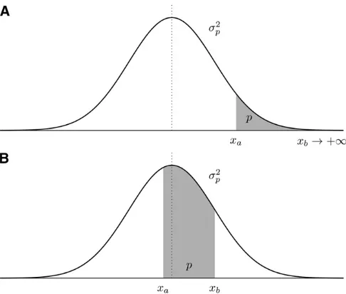
the percentage of cases when one or both parents of the top-ranking offspring individuals belong to the corresponding truncated p fraction of the P population (Figure 1a). It should be emphasized that the parents inPmate randomly,

producing theF1offspring, and, therefore, this scenario

dif-fers from conventional truncation selection as the topp pro-portion of the parental population were not“selected”and constrained to mate among themselves. Rather, both top-ranking parents and offspring are only“inspected”to calcu-later. We postulate thath2_{may be calculated based on the}

three parameters:p,r, ands2 p:

It follows that the case for truncation selection (Figure 1a) can be generalized to the case of a two-sided truncation with

X2 ðxa;xbÞ(Figure 1b).

This approach differs from classical methods to estimateh2

in that it does not rely on the degree of resemblance among relatives or variance component decomposition. This method resembles a realizedh2 _{estimate, but it differs from classical}

realizedh2_{because it is applicable to panmictic populations,}

and does not require experimentally controlled crosses among selected parents. This strategy was motivated by a mathemat-ical analysis of the effect of phenotypic preselection on reducing contamination rate in seed orchards of forest trees (Lstib˚urek

et al.2012). This approach is similar to methodology developed to estimateh2_{for binomial (threshold) traits (Crittenden 1961;}

Falconer 1965), but here we are concerned with normally dis-tributed quantitative traits.

Mathematical derivation

We begin with the derivation of the more general two-sided truncation scenario. LetXNðm;s2

pÞandX2 ðxa;xbÞ;then

we follow the transformation properties of the normal distri-butionXNð0;1ÞandX2 ða;bÞ;where

a¼ xa2m

sp ;

b¼ xb2m

sp :

(1)

Figure 1 Normal distribution of a quantitative trait (identical in thePand

F1populations). The truncation proportionp(gray area) is delimited by the left (xa) and right (xb) truncation points, respectively. Two scenarios

For given xa and xb; one may calculate the area p of the

truncated distribution (Figure 1) as

p¼FðbÞ2FðaÞ; (2)

whereFðaÞandFðbÞare the cumulative distribution func-tions (cdf) of the normal distribution Nð0;1Þ: The corre-sponding truncated distribution is then (Johnsonet al.1994)

E½XP ¼mþisp;

Var½XP ¼ ð12kÞs2

p: (3)

The selection intensity (i) is then defined as

i¼2fðbÞ2fðaÞ

FðbÞ2FðaÞ; (4)

wherefðaÞandfðbÞare the probability density functions of the standardized normal distribution, and the coefficientkis

k¼bfðbÞ2afðaÞ

FðbÞ2FðaÞ þ

fðbÞ2fðaÞ

FðbÞ2FðaÞ !2

: (5)

We can trace the likelihood that one or both parents of a given offspring originate from the truncated subsetp. The number of parents satisfying this origin is binomially distributed as

Y1Bið1;pÞ when tracking one side of the parentage, and Y2Bið2;pÞwhen tracking both sides of the parentage. In these

cases, the respective likelihoods that one parent or both parents, respectively, originate frompare enumerated in Table 1.

Then, for one of the two above scenarios, the expected value and variance of the offspring inF1 are

E½XF₁ ¼mþBih2_s p;

Var½XF1 ¼

120:5Bkh4s2p: (6)

where the coefficientBis provided in Table 1.

Letp* be the proportion of the above offspring (Equation 6) belonging to the intervalða;bÞofF1:In our remaining analyses,

we utilize the central limit theorem,i.e., the normal approx-imation of the above distribution. Utilizing the same trans-formation properties of the normal distribution (Equation 1), the areap* is given by

p*¼F b2Bih

2

ffiffiffiffiffiffiffiffiffiffiffiffiffiffiffiffiffiffiffiffiffiffiffiffiffi

120:5Bkh4

p

!

2F ffiffiffiffiffiffiffiffiffiffiffiffiffiffiffiffiffiffiffiffiffiffiffiffiffia2Bih2

120:5Bkh4

p

!

: (7)

LetNbe the size of theF1population. Then,NF1is the number

ofF1individuals in the intervalðxa;xbÞ:NPðYÞis the subset of NF1where the parent(s) originate from the intervalðxa;xbÞin

P, according toY. Next, we introduce a variabler, the relative frequency of offspring in the truncated proportion inF1with

parent(s) originating from the truncated proportion of P, according toY, where

r¼NPðYÞ

NF₁ : (8)

Next, we utilize the earlier binomial expansion, and

r¼NPðYÞ NF1

¼Np*PðYÞ

Np ¼

p*PðYÞ

p : (9)

With the knowledge ofpandr, we can ascertain the unknown

p*;thus

pr PðYÞ¼F

b2Bih2 ffiffiffiffiffiffiffiffiffiffiffiffiffiffiffiffiffiffiffiffiffiffiffiffiffi

120:5Bkh4

p

!

2F ffiffiffiffiffiffiffiffiffiffiffiffiffiffiffiffiffiffiffiffiffiffiffiffiffia2Bih2

120:5Bkh4

p

! : (10)

Therefore,h2 _{is the implicit function ofr,p, ands}2

p:(Additional

variables in the equation are all functions of these three input parameters.) The above formulation is general, and could be used with mathematical solver software to calculate an estimate ofh2_:

Computer code to solve forh2 _{using Equation 10 written in R}

language (R Core Team 2013) is provided in a public repository (Lstib˚urek 2017). Next, we derive analytical solutions (i.e., de-terministic equations) to estimateh2_{for two specific cases.}

Case 1: centered two-sided truncation:Provided bothxaand

xbare symmetrically allocated around the mean ofPandF1;h2is

calculated as (see Supplemental Material,File S1for derivation)

h2¼ ffiffiffi

2

p

jQj

Q2_2a2 Bk

1 2

; (11)

whereQ¼F21ð0:52pr=2PðYÞÞ:

Case 2: right-sided truncation:Whenxb/þN(Figure 1),

one may calculateh2_{as (seeFile S1for derivation)}

h2¼2aBi6

4a2_B2_i2_222B2_i2_þBQ92_ka2_2Q9212 ð2B2_i2_þBQ92_kÞ ;

(12) whereQ9¼F21ð12pr=PðYÞÞ:There are two solutions of the above equation, and verification using Equation S1.7 pro-vides the unique one.

Variance of the h2estimate:The SE associated with the general

h2_{estimate (Equation 10) is (seeFile S1for derivation)}

SE h2¼

120:5h4_kB32

jfðbÞð2iBþ0:5h2_{bkBÞ2fðaÞð2iBþ0:5h}2_akBÞj

3 p

PðYÞ

ffiffiffiffiffiffiffiffiffiffiffiffiffiffiffiffi rð12rÞ

p 1

ffiffiffi n

p ;

(13)

Table 1 Likelihoods and coefficients

PðYÞ B

Y1¼1 p 0.5

Y2¼2 p2 1

where nis the number of progeny inp,h2_{6¼0 under}

sym-metric two-sided truncation, andaandbare

a¼ a2Bih 2

ffiffiffiffiffiffiffiffiffiffiffiffiffiffiffiffiffiffiffiffiffiffiffiffiffi

120:5Bkh4

p ;

b¼ b2Bih 2

ffiffiffiffiffiffiffiffiffiffiffiffiffiffiffiffiffiffiffiffiffiffiffiffiffi

120:5Bkh4

p :

(14)

The SE of theh2_{estimate for the scenario of right-sided}

trun-cation (Equation 12) is

SE h2¼

120:5h4kB32 j2fðaÞð2iBþ0:5h2_akBÞj

p PðYÞ

ffiffiffiffiffiffiffiffiffiffiffiffiffiffiffiffi rð12rÞ

p 1

ffiffiffi n

p :

(15) Equations 13 and 15 are both products of two components, where thefirst (leftmost) is associated with the type and in-tensity of truncation, and the second (rightmost) depicts the variance ofr, including the sample sizen.

Utilizing the mathematical derivation outlined above, we claim that estimates ofh2_{and the corresponding SE are}

as-ymptotically unbiased.

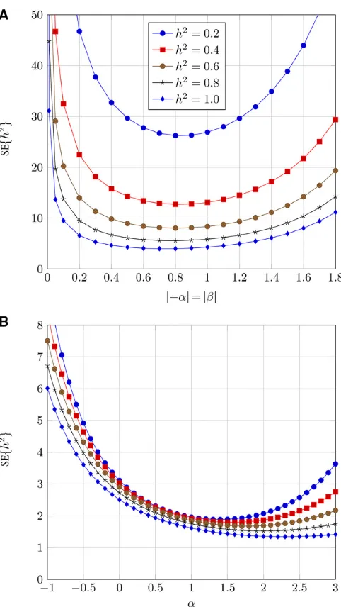
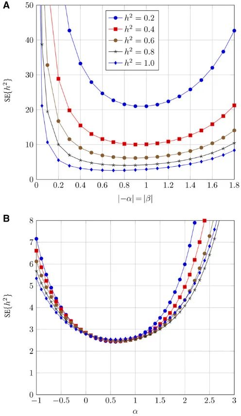
The SE are provided for the two likelihoods (Y1¼1 and Y2¼2) and one- or two-sided truncations in Figure 2 and

Figure 3. The SE is comparable to existing methods, i.e., regression analysis; thus, the number of samples providing reliable estimate ofh2 _{is in the magnitude of“hundreds.”}

Data availability

The authors state that all data necessary for confirming the conclusions presented in the article are represented fully within the article.

Computer simulation

As noted above, our formal theoretical derivations using normal distributions are not strictly true with truncation. Therefore, we verified our analytical approach by stochastic simulation, whereh2_{was estimated for a hypothetical}

pan-mictic population as follows. Additive polygenetic effects of 10,000 unrelated and noninbred parental individuals were sampled from the normal distributionNð0;s2

aÞ;assuming the

infinitesimal genetic model. The environmental deviation was drawn from Nð0;s2

eÞ: Subsequently, 10,000 individual

offspring were generated. Parents were randomly mated and polygenic additive genetic values in offspring were drawn from

Nða;0:5s2

aÞ; where a is the respective midparental additive

genetic value. The environmental deviation was assigned as for the parental population.

Next, 1000 offspring with trait’valuesX2 ðxa;xbÞ were

inspected, and r was calculated for each of the likelihood scenarios ðY1¼1;Y2¼2Þ by evaluating the trait value of

parents.h2_{was then estimated by solving Equation 10.}

Sim-ulations were repeated for 100 independent stochastic itera-tions, and means and variances were calculated across all runs, and compared to the true parameters2

a=s2p:Computer

code to perform the simulation written in R language is provided in a public repository (Lstiburek 2017).˚

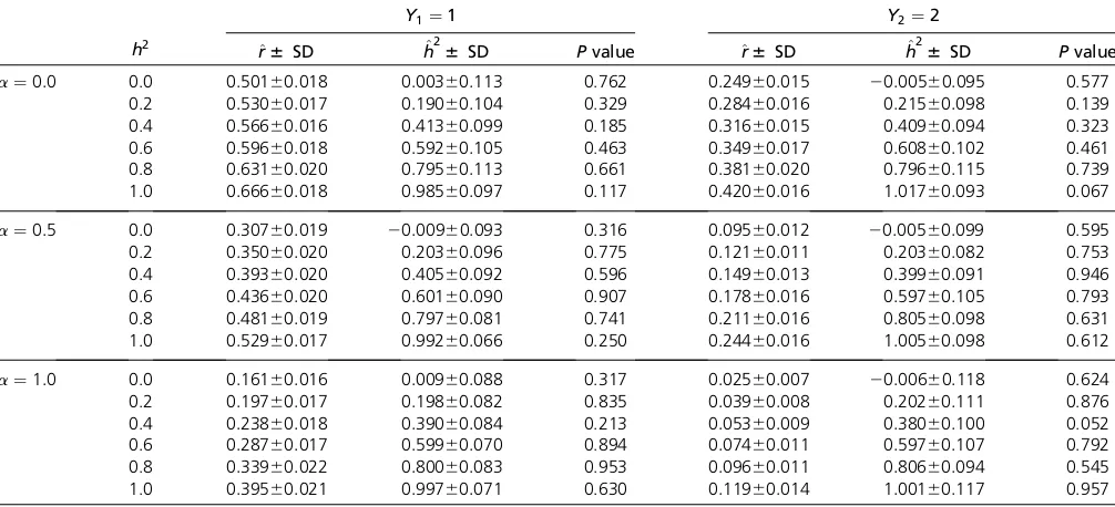
The simulations showed that the normal approximation of the assumed F1 distribution (Equation 6) is justified,

since the expected value ofh2_{estimates were nearly}

iden-tical to the true parameters across 100 independent sto-chastic simulations for all assumed scenarios (h2_{from 0 to}

1), a¼0, 0.5, and 1, andb¼ þNacross the two likeli-hoods (Table 2).

Demonstration using human height

We used Galton’s well-known dataset of human heights (Galton 1886). The dataset includes 205 families with adult heights of 934 children, in family sizes range from 1 to 15 children. The

Figure 2 SE of theh2_{estimate (SEfh}2_{g) forðY}

dataset is publicly available as R package (Friendly et al.

2017), and we used it for our demonstration. Hanley (2004) analyzed this original dataset, and he was partic-ularly addressing the issue of Galton’s original adjustment for the gender,i.e., all heights of women were multiplied by 1.08. First, we reproduced Hanley’s calculations, and received identical estimates of the regression coefficientb

(Table 1 in Hanley 2004). Then, we considered Galton’s original adjustment, where ^b = 0.71 (regression of the heights of children on midparent values), which provides the direct estimate of h2_{:We used restricted}

maximum-likelihood approach to verify thesefindings using the an-imal genetic model in ASReml (Gilmour et al. 2009), where the random pedigree effect was the single factor in the model.

As expected, we received identical estimate ofh2 _¼0:71

and SE of 0.04 (identical to the SE of bin our regression analysis). Then, we followed our approach and analyzed offspring in the right site of the distribution (truncation.0.5 of the standardized normal distribution),i.e., approximately one-third of Galton’s dataset. We assumed tracking one side of the parentage, as it leads to the lower SE (compare Figure 2b and Figure 3b). All children values (adjusted dataset by Galton) were sorted. Then we started assessing the tallest child and compared, whether the mother’s height was above the same truncation. We recorded all positive values (as 1s); the sum for one parentage across all truncated children (278) was 122 and for the second parentage 137. We aver-aged these values and divided the result by 278 and obtained the value of ^r¼0:47: Then, assuming Equa-tion 10, we estimatedh2_{to be 0.73 with SE 0.07 (the error}

is actually,0.07 since we averaged two^rvalues).

Discussion

The main methodological message of this study is that it is possible to estimateh2_{within a panmictic population without}

a planned experiment, and without performing a complete pedigree reconstruction across the entire phenotypic distri-bution of parental and offspring populations in order to im-plement traditional variance component estimation. Our approach provides a way to estimateh2 _{by genotyping only}

a small proportion of the parental and offspring populations (e.g., the right-hand tail of the distributions), and estimating the proportion of that subset of offspring that arose from that subset of parents. It is thus an estimate of realizedh2_;derived

from quantifying the relatedness among exact phenotypic subsets of parental and offspring populations.

Much formal quantitative genetics theory follows a simple biological principle: the additive genetic value of an offspring is the midparent additive genetic value plus the Mendelian sampling term. The phenotype is further determined by add-ing an error term, where each offspradd-ing is allocated a random environmental variate from the corresponding normal dis-tribution. This reasoning is the key to understanding the approach presented here: parents are sampled from the populationPindependently and randomly (with replace-ment) and they form the corresponding normal distribu-tion F1: Thus, all parental combinations occur with the

same probability,i.e., random mating. Variation in family sizes is therefore an integral part of the model and the model is thus experimentally tailored to truly panmictic populations.

The classical methods for estimatingh2 _{using offspring–}

parent or offspring–midparent regression, and ANOVA-based approaches promote experimental efficiency by artificially manipulating the family structure with respect to the actual family numbers and sizes, so that the SE are minimized. Sim-ilarly, we can assess the experimental parameters a,b, and progeny sample sizenthat minimize SEfh2_{gdetermined by}

our method. An extension of the classical methods is to use

Figure 3 SE of theh2_{estimate (SEfh}2_{g) forðY}

restricted maximum likelihood approach (Patterson and Thompson 1971) for variance decomposition, both in syn-thetic and wild populations, provided variance-covariance of phenotypic records is specified by use of a relationship matrix (i.e., complete pedigree linking respective records to the base population), and assumptions of the infinitesimal model hold (Sorensen and Kennedy 1984).

The approach outlined here is different, as it allowsh2_{to be}

estimated based on the truncated, rather than a random, subset, thus pedigree relationship is needed only within the truncated subsets of the distribution. Regression based on a truncated subset produces a biasedh2 _{estimate because the}

entire population sample (and particularly extreme values) are needed to estimate the slope of the regression line. It is possible to modify the regression procedure where most of the effort is applied to families of parents with phenotypes at both ends of the distribution, which would yield a precise estimate (Hill 1990). The increase in efficiency is because parents with phenotypes near the mean provide little infor-mation on the slope of the regression. However, we show here that h2 _{can be estimated based on either phenotypes}

near the mean, or from phenotypic observations in only one extreme of the distribution. These arbitrary truncations ap-plied to the normal distribution are different from the tradi-tional approaches and could offer experimental scenarios that have not yet been considered in genetic studies. Our approach is based on determining the means and variances ofPandF1populations and the relative frequency of offspring

in the truncated proportion in F1 with parent(s) originating

from the truncated proportion ofP. Provided the panmictic assumptions hold, our approach is therefore experimentally very simple and general.

First, it is clear that the precision of h2 _{estimate will be}

much higher for one-sided truncation than for centered two-sided truncation. Comparing Figure 2 and Figure 3, we see that the SEfh2_{gfrom centered two-sided truncation are on}

the order of 5–103those from one-sided truncation. In fact, close inspection of Equations 13 and 15 reveals that the min-imum SEfh2_{gis obtained from the one-side truncation}

sce-nario. Next, we can assess the optimuma, the standardized truncation point. For Y1 ¼1 (tracking only one side of the

parentage), the optimumawill generally be between 1 and 2 SD (Figure 2b). ForY2¼2 (tracking both sides of the

par-entage), the optimumais between 0 and 1 SD across a range ofh2_{(Figure 3b).}

We now consider how this method could be implemented in practice. Thefirst step is to calculate phenotypic means and variances in both thePandF1populations. The second

step is to genotype a random sample of individuals in the right-truncated tail of theF1(sayn¼500 in the phenotypic

range froma¼1:5 SD above the mean up tob¼ þN) as well as parents belonging to the equivalent phenotypic range in thePpopulation. The pedigree can then be inferred from these genotype data. The coefficientrcan then be calculated by eval-uating ifY1 ¼1;i.e., tracking one side of the parentage. We can

then use Equation 12 to calculateh2_{:If the trueh}2_¼0:6;then

the SEfh2_{g ¼1:69431=}pffiffiffiffiffiffiffiffiffi_{500¼0:076 (Equation 15 and}

Figure 2b). Ifais 2 SD above the mean, the corresponding SEfh2_{g ¼1:69131=}pffiffiffiffiffiffiffiffiffi_{500¼0:076; i.e., identical, but the}

amount of genotyping effort in the parental population is greatly reduced. Note that traditional regression on one parent provides SEfh2_{g ¼2=}pffiffiffiffiffiffiffiffi_{500¼0:089, and that on midparent}

values gives SEfh2_{g ¼}pffiffiffiffiffiffiffiffiffiffiffiffiffiffiffiffiffiffi_{ð2=500Þ¼0:063 (Falconer and}

Mackay 1996).

Table 2 Results of computer simulations

Y1¼1 Y2¼2

h2 _{^r6 SD h^}2_{6 SD Pvalue ^r6SD ^h}2_{6 SD Pvalue}

a¼0:0 0.0 0:50160:018 0:00360:113 0.762 0:24960:015 20:00560:095 0.577 0.2 0:53060:017 0:19060:104 0.329 0:28460:016 0:21560:098 0.139 0.4 0:56660:016 0:41360:099 0.185 0:31660:015 0:40960:094 0.323 0.6 0:59660:018 0:59260:105 0.463 0:34960:017 0:60860:102 0.461 0.8 0:63160:020 0:79560:113 0.661 0:38160:020 0:79660:115 0.739 1.0 0:66660:018 0:98560:097 0.117 0:42060:016 1:01760:093 0.067 a¼0:5 0.0 0:30760:019 20:00960:093 0.316 0:09560:012 20:00560:099 0.595 0.2 0:35060:020 0:20360:096 0.775 0:12160:011 0:20360:082 0.753 0.4 0:39360:020 0:40560:092 0.596 0:14960:013 0:39960:091 0.946 0.6 0:43660:020 0:60160:090 0.907 0:17860:016 0:59760:105 0.793 0.8 0:48160:019 0:79760:081 0.741 0:21160:016 0:80560:098 0.631 1.0 0:52960:017 0:99260:066 0.250 0:24460:016 1:00560:098 0.612 a¼1:0 0.0 0:16160:016 0:00960:088 0.317 0:02560:007 20:00660:118 0.624 0.2 0:19760:017 0:19860:082 0.835 0:03960:008 0:20260:111 0.876 0.4 0:23860:018 0:39060:084 0.213 0:05360:009 0:38060:100 0.052 0.6 0:28760:017 0:59960:070 0.894 0:07460:011 0:59760:107 0.792 0.8 0:33960:022 0:80060:083 0.953 0:09660:011 0:80660:094 0.545 1.0 0:39560:021 0:99760:071 0.630 0:11960:014 1:00160:117 0.957

We will now explain how (in theory) Galton could have utilized our approach to collect the dataset. First, he would need estimates of the mean and variance of the trait in a population (we assume that records would be available without much investment). Then, he could choose to measure 278 children

.0.5 SD above the average and check in the same manner parental values. With unknown parentage, pedigree assem-bly could be reduced from 934 to 278 children, reducing significantly the cost of sample collection, DNA extraction, and genotyping. Reduced sample size could also be possible with regression analysis, assuming a random sample (of say 278 children) across the entire range of the distribution with higher SE. However, the main methodological message of the current study is that we can estimateh2_{based on the}

tail of the distribution. Regression in such a case would re-sult in a biased estimate (e.g., the same truncated dataset would produce^bestimate¼^h2 _{estimate¼0:31).}

We could speculate that our approach is less sensitive to the presence of outliers as all individuals above the truncation contribute equally tor. In regression analysis, outliers are most influential in either extreme of the distribution with respect to the slope of the regression line. In the ASReml analysis (Gilmour

et al.2009) that we performed on the same dataset, three pos-sible outliers were suggested. When we removed these from the analysis,h2 _{changed to 0.72 (SE was identical).}

In summary, we propose an alternative formulation ofh2_:

Under the assumptions of Hardy-Weinberg equilibrium, the

h2 _{of a quantitative trait in a given population is directly}

related to the likelihood of a phenotypic subset of parents passing their respective alleles onto the corresponding phe-notypic subset of offspring. Future work is needed to com-pare the efficiency of this method to other existing methods; to estimate nonadditive genetic effects; to assess robustness with respect to the genetic architecture of the trait; and to assess the sensitivity of the approach to assumptions of Hardy-Weinberg equilibrium.

Acknowledgments

We thank Jan Stejskal for his assistance with the data analysis. M.L. is supported by grant“EXTEMIT - K,”No. CZ.02.1.01/0.0/ 0.0/15_003/0000433financed by Operational Programme Re-search, Development, and Education (OP RDE). The research of J.P. is supported by the Czech Science Foundation, project No. 15-00243S. G.R.H. is supported by Camcore, Department of Forestry and Environmental Resources, North Carolina State University.

Literature Cited

Aykanat, T., S. E. Johnston, D. Cotter, T. F. Cross, R. Pooleet al.,

2014 Molecular pedigree reconstruction and estimation of

evolutionary parameters in a wild Atlantic salmon river system with incomplete sampling: a power analysis. BMC Evol. Biol. 14: 1.

Crittenden, L. B., 1961 An interpretation of familial aggregation

based on multiple genetic and environmental factors. Ann. N. Y.

Acad. Sci. 91: 769–780.

de los Campos, G., D. Sorensen, and D. Gianola, 2015 Genomic

heritability: what is it? PLoS Genet. 11: e1005048.

Falconer, D. S., 1965 The inheritance of liability to certain

dis-eases, estimated from the incidence among relatives. Ann. Hum.

Genet. 29: 51–76.

Falconer, D. S., and T. F. C. Mackay, 1996 The Introduction to

Quantitative Genetics, Ed. 4. Longmans Green, Harlow, UK.

Friendly, M., S. Dray, H. Wickham, J. Hanley, D. Murphy et al.,

2017 HistData: data sets from the history of statistics and data

visualization. R package version 0.8–2, dataset’GaltonFamilies’.

Available at: https://cran.r-project.org/web/packages/HistData/

HistData.pdf. Accessed September 25th, 2017.

Galton, F., 1886 Regression towards mediocrity in hereditary

stat-ure. J. Anthropol. Inst. G. B. Irel. 15: 246_–263.

Gilmour, A. R., B. Gogel, B. Cullis, R. Thompson, D. Butleret al.,

2009 ASReml User Guide Release 3.0. VSN International Ltd, Hemel Hempstead, UK.

Hanley, J. A., 2004 “Transmuting” women into men: Galton’s

family data on human stature. Am. Stat. 58: 237–243.

Hill, W. G., 1990 Considerations in the design of animal breeding

ex-periments, inAdvances in Statistical Methods for Genetic Improvement

of Livestock(Advanced Series in Agricultural Sciences), chapter 4,

pp. 59–76, edited by D. Gianola, and K. Hammond.

Springer-Verlag, Berlin.

Johnson, N. L., S. Kotz, and N. Balakrishnan, 1994 Continuous

Uni-variate Distributions. Wiley Series in Probability and Mathematical Statistics, Ed. 2. John Wiley & Sons, New York.

Lstiburek, M., 2017˚ Estimating realizedh2 _{in panmictic}

popula-tions, computer code. Available at:https://github.com/mlstiburek/

genetics-heritability.git. Accessed September 25th, 2017.

Lstib˚urek, M., J. Klápˇstˇe, J. Kobliha, and Y. A. El-Kassaby, 2012 Breeding

without breeding: effect of gene_flow on_fingerprinting effort.

Tree Genet. Genomes 8: 873_–877.

Lynch, M., and B. Walsh, 1998 Genetics and Analysis of Quantitative

Traits, Vol. 1. Sinauer, Sunderland MA.

Patterson, H. D., and R. Thompson, 1971 Recovery of inter-block

information when block sizes are unequal. Biometrika 58: 545–554.

R Core Team, 2013 R:A Language and Environment for Statistical

Computing. R Foundation for Statistical Computing, Vienna.

Sorensen, D., and B. Kennedy, 1984 Estimation of genetic

vari-ances from unselected and selected populations. J. Anim. Sci.

59: 1213–1223.

Yang, J., B. Benyamin, B. P. McEvoy, S. Gordon, A. K. Henderset al.,

2010 Common SNPs explain a large proportion of the

herita-bility for human height. Nat. Genet. 42: 565–569.