Adaptive boundary element method.

University of Windsor University of Windsor

Scholarship at UWindsor

Scholarship at UWindsor

Electronic Theses and Dissertations Theses, Dissertations, and Major Papers

1-1-1991

Adaptive boundary element method.

Adaptive boundary element method.

Weiwei Sun

University of Windsor

Follow this and additional works at: https://scholar.uwindsor.ca/etd

Recommended Citation Recommended Citation

Sun, Weiwei, "Adaptive boundary element method." (1991). Electronic Theses and Dissertations. 6150. https://scholar.uwindsor.ca/etd/6150

This online database contains the full-text of PhD dissertations and Masters’ theses of University of Windsor students from 1954 forward. These documents are made available for personal study and research purposes only, in accordance with the Canadian Copyright Act and the Creative Commons license—CC BY-NC-ND (Attribution, Non-Commercial, No Derivative Works). Under this license, works must always be attributed to the copyright holder (original author), cannot be used for any commercial purposes, and may not be altered. Any other use would require the permission of the copyright holder. Students may inquire about withdrawing their dissertation and/or thesis from this database. For additional inquiries, please contact the repository administrator via email

NOTE TO USERS

This reproduction is the best copy available.

ADAPTIVE BOUNDARY ELEMENT METHOD

BY WEI WEI SU N

A Dissertation submitted to the

Faculty of Graduate Studies and Research through the Department of

Mathematics and Statistics i n Partial Fulfillment of the requirements for the Degree

of Doctor of Philosophy at the University of Windsor

UM I Number: D C 5 3 2 6 0

INFO RM ATIO N T O USERS

The quality of this reproduction is dependent upon the quality of the copy

submitted. Broken or indistinct print, colored or poor quality illustrations

and photographs, print bleed-through, substandard margins, and improper

alignment can adversely affect reproduction.

In the unlikely event that the author did not send a complete manuscript

and there are missing pages, these will be noted. Also, if unauthorized

copyright material had to be removed, a note will indicate the deletion.

UMI Microform D C 5 3 2 6 0 Copyright 2009 by ProQuest LLC

All rights reserved. This microform edition is protected against unauthorized copying under Title 17, United States Code.

ProQuest LLC

789 East Eisenhower Parkway P.O. Box 1346

Ann Arbor, Ml 48106-1346

7 ? < ? - & 7 7 7

Abstract

T h i s I h A s i a i s d « v o i « d t o i h « s t u d y o f t h * a d a p t i v e

b o u n d a r y element method, a subject which has been explored i n t e n s i v e l y during the last f e w years. In this thesis, a systematic simulation for the adaptive r - m ethod is presented for the Laplace's e q u ation with constant, linear and quadratic elements and the equations of linear elast i c i t y with linear and quadratic elements. The stability, singularity, advantages, disadvantages a n d limitations of the a l g orithm a r e explored. Based on the present discussions, a n e w adaptive h-r a l g o r i t h m is developed. In this combined algorithm, the residual error used as an error indicator is m i nimized suc h that the m esh achieves asymptotic optimality. Simultaneously, the number of grid points is a d a p t i v e l y increased to meet a s p e cified user tolerance. The a l g o r i t h m is s u c c e s s f u l l y used in solv i n g Laplace's equation and Navier's e q u a t i o n of linear elasticity.

i v

ACKNOWLEDGEMENT

I would like to express m y gratitude to m y supervisor, Professor N. G. Zamanl for suggesting the topic of this dissertation and for his generous help throughout m y studies at University -of Windsor. His encouragement and kindness have been a great support which I will remember forever.

vi

T A B L E O F C O N T E N T S

A b s t r a c t * •;...i v

D e d i c a t i o n ... ... v

A c k n o w l e d g e m e n t ... vi

Chapter O n e I n t r o duction 1.1 B a c k g r o u n d ... 1

1.1.1 Adapti ve methods 1 . 1 . 2 Optimal mesh 1 .1.3 Grading function 1. 2 C a r e y and Dinh's a l g o r i t h m ... 7

1. 3 Outl i n e of the Thesi s ...12

Chapter T w o Th e Optimal M e s h A l g o r i t h m C r — method^ 2.1 I n t r o d u c t i o n ... IS 2. 2 Error I n d i c a t o r ... 1©

2 . 3 A d a p t i v e Optimal M esh A l g o r i t h m ... 20

2.4, P o t e n t i a l ... 23

2 . 3 Linear E l a s t i c i t y ... 43

2. O Concl usi o n ... 30

Chapter T h r e e A n A d a ptive h —r B o u n d a r y Element A l g o r i t h m For the Lapl a c e E q u a t i o n 3.1 I n t r o d u c t i o n ... 09

3. 2 T runcation Error I n d i c a t o r ... 70

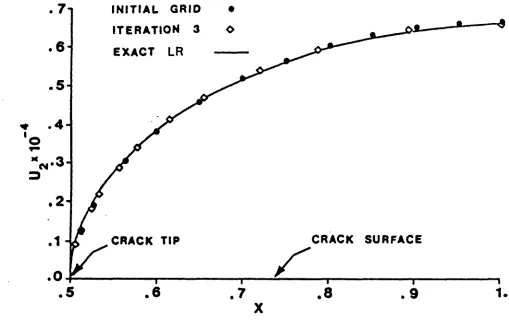
3.4 Numerical R e s u l t s ...81

3.5 C o n c l u s i o n ... 90

Chapter Four A n Adaptive h-r Algorithm For the Equations of Linear Elasticity 4.1 I n t r o d u c t i o n ... Qi 4.2 Truncation E r r o r ...91

4.3 The Adaptive A l g o r i t h m ... 99

4.4 Numerical R e s u l t s ...104

4.5 Conclusion ... 112

Chapter Five Stability and Singularity 5.1 I n t r o d u c t i o n ... 113

5.2 Continuous Distribution F u n c t i o n s ...117

5 .3 Singular Distribution F u n c t i o n s ... 120

Chapter Six C o n c l u s i o n ...132

Chapter S e v e n Appendix I 7.1 The Proof of Theorem 2 . 1 ...135

7.2 The Extension of Mean Value T h e o r e m ... 141

7.3 The Basic Formulas in Boundary Element Methods ...142

7.4 An Interpolation Error Analysis of the Cauchy Mean Value I n t e g r a l ... 149

Chapter Eight Appendix II

8.1 Fundamental Equations in Linear Elasticity

vi i i

... 157 8.2 Tl»e Analytic Solution of Example 2 . 3 ... 158 8.3 The Analytic Solution of Example 2 . 4 ... 159 8.4 The Formula for Stress Intensity F a c t o r 161 8.5 The Analytic Solution of Example 4 . 1 ... 163

Chapter One Introduction

1.1 Background

1.1.1 Adaptive Methods

Adaptive methods have become important tools in the numerical solution of o r d i n a r y and partial differential equations m a i n l y due to the need for ext e n s i v e analysis of computer output p a r t i c u l a r l y when an initial solution is not satisfactory. It is v e r y de s i r a b l e to incorporate automatic C adaptive!) decision ma k i n g algorithms into software such as finite element. fi n i t e d ifference and bo u n d a r y element programs. A d a ptive techniques have been used for a long time in the s t e p s i z e control of o r d i n a r y differential equations. T h e recent advances in Expert Systems and Artificial Intelligence have triggered considerable research in the area of adaptive algorithms £4. 42.493. Four recent conferences on this topic reflect the major activities undertaken b y mathematicians and engineers in this area £6,7,20,323.

In the context of the numerical s o l u t i o n of partial differential equations, an adaptive method is an automatic adjustment of certain parameters based o n the approximate solution obtained. In general, this adjustment takes place o n l y after an initial solution has been obtained in parts of

1

the domain where the discretization is poor as identified b y

an a /posteriori error indicator and therefore, such methods

are iterative in nature. Most of the work in this area is based on local methods. For this reason, our discussion is implicitly directed to such techniques. The term adjustment, which is fundamental in an adaptive method, has been applied in three different contexts as follows:

1. h-method Cmultigrid, local refinement and h-version); 2. p —method;

3. r —method Coptimal mesh and mesh redistribution^.

These concepts have been used in some commercial codes [2,3,8,28,34,35,663. In the h-method. the number, of nodal points in the discretization is increased in the whole domain or only in the areas of large solution gradients. This procedure is perhaps the oldest technique for improving the quality of the numerical solution. In the p-method. the number of nodal points is kept fixed but the degree of the approximating polynomial is increased. The concept of p — method is still under intensive investigation. Finally, the r-method is the least explored subject in the numerical solution of partial differential equations among the three algorithms. In the r-method, the number of nodal points and the degree of the approximating polynomial are kept fixed but the positions of the nodes are altered. Naturally, there should be a large concentration of nodal points in regions of steep gradients.

dependent upon the error indicator. In most investigations* the numerical di s c r e t i z a t i o n error in solv i n g differential equations is used as an error indicator. Because of the rigorous theoretical foundations, most a d a p t i v e techniques hav e been s u c c e s s f u l l y and p r i m a r i l y applied t o finite element methods. Unfortunately* the b o u n d a r y element methods CBEMD d o not benefit f r o m suc h rigour and* therefore, there is more heuristics involved. This is perhaps because of a fundamental diffe r e n c e between differential and integral equations. It is well k n o w n that elliptic differential operators are local in nature whereas the integral operators arising i n regular elliptic b o u n d a r y v alue problems d o not possess this property. Recently* s o m e theoretical analysis on the local character of the b o u n d a r y integral equations was presented b y Wendl a n d and Yu £643* where the b o u n d a r y integral equations were c o n s i d e r e d as a p s e u d o —differential operator acting on th e boundary. T h e exi s t e n c e of residual e stimates of the global error has a lso bee n d e m o n strated b y Rank £403 for the G a l e r k l n b o u n d a r y element method. Thus, s ome of th e results obtai n e d for the a d a p t i v e fin i t e element method h ave b e e n t r a n s f e r r e d to t h e a d a ptive b o u n d a r y e lement method. Until r e c e n t l y most of the research i n adaptive -boundary elements has focused on th e h —method* such as the results p r e sented b y Rencis an d Mu l l e n £43], Rencis £44], Wendland a n d Yu £643. Rank £41]. Guiggiani £23] and Gomez-Lera, Cer r o l a z a a n d Alar c o n £213. V e r y f e w articles have dealt with the a d a p t i v e p —met h o d £1*14*38.613 and I— method £13*29,573. In general* th e latter is b ased o n a

3

stricter error expression. The error analysis known in the boundary element method is still not precise enough in spite of the theoretical results and error estimates for boundary integral equations presented b y Wendland C62.633, Hisao C25] and Costabel a n d Stephen Cl63. There are numerous other

r e f e r e n c e s b u t d u e t o l a c k o f s p a c e o n l y s o m e a r e l i s t e d

here C21.27.31.32,33.45,46.47,48.51 .53.55,603 .

Recently, some combined adaptive algorithms have been explored. Theoretically, a n y combination of the h, p and r methods can produce an adaptive algorithm. The onl y combined algorithms known in the literature are the adaptive h-p method used in finite elements b y Gui and Babuska C223 and boundary elements b y Guo, von Petersdorff and Stephen C243 and our adaptive h-r method to be presented in chapters 3 and 4.

1.1.2 Optimal Mesh

At the e a r l y stages of the development of digital computers. most algorithms for numerical solution of differential equations employed uniform meshes. As o n e of the e arly pioneers. Brown CQ3 used a non-uniform mesh in solving a nonlinear two-point bound a r y value problem where the truncation error o n the n on-uniform mesh was of higher o r d e r .

expressed as

rain RCu,x.} C l . 1.1}

subject, to : x < x < < x * ueH

J O 1 N N

where RCu.x^} is an obj e c t i v e f u n ction d e n o t i n g an error or a physical indicator. H is an N —dimensional space of the solutions of the p r o b l e m and u is a s o l u t i o n with respect to the mesh Cx^}. When the n e c e s s a r y conditions for minimization are used, the optimal mesh is chara c t e r i z e d b y the s y s t e m of nonlinear equations.

5^ - * o i = i . a , . . . , M , c i . l . a }

(7U.

= O J * 1 , 2 N. C l . 1.3} i

where M is the number of nodal unknowns and N is the number of grid points. In general. Cl.1.1} is a nonlinear pr o g r a m m i n g p r o b l e m w i t h c onstraints w h i c h cannot be solved analytically. A l t h o u g h the s t a n d a r d co n s t r a i n e d nonlinear programming algorithms w e r e p r o p o s e d to s o l v e the optimal mesh p r o b l e m £11,52,633, numerical c o m p u t a t i o n can be v e r y expensive. In these references, RCu.x} is defi n e d as the e n e r g y functional a l l o w i n g bot h the nodal values and coordinates to enter as unknowns. A practical method is to t r y to uncouple equations C l . 1.2} and C l . 1.3} and then s o l v e t hem iteratively.

1 .1.3 G r a d i n g Function

T h e concept of the grad i n g f u n c t i o n was o r i g i n a l l y

S

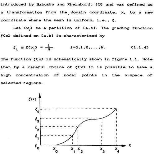
introduced b y Babuska and Rheinboldt C53 an d was defined as a transformation f r o m the domain coordinate, x, to a n e w coordinate where the mesh is uniform, i . e. , £.

Let ■CsO' a. partition of Ca,b3. The grading function £Cx3 defined on Ca,bl is characterized b y

s ?Cx.) - -4r- i = 0 , 1 , 2 N. Cl.1.40

i t N

The function £CxD is s c h e matically shown in figure 1.1. Note that b y a careful choice of £C xD it is possible to hav e a high concentration of nodal points in the x —s pace of selected regions.

Fig. 1.1 Mapping f r o m x to £ through the grading function

In most theoretical studies, the o b j ective function RCu,x.Z) in section 1 . 1 . 2 is assumed to be an error indicator in the numerical solution of the differential equation. R c an therefore be expressed as a function of the solution uC xD and h., where lv is the element length, i.e. , h.«x. —

expressed in terms of th e grad i n g function £Cx3 as follows.

min RCu.?3 C l . 1.53

Z

ueH

N

The above p r o b l e m is on e of calculus of variations and. in s o m e cases. closed f o r m solutions c a n b e obtained. The algorithms derived in this thesis will f o l l o w s u c h a concept.

1.2 C a r e y and D±nh*s Method

In 1685. C a r e y and D i n h ti23 p r esented a n analysis of optimal mesh and optimal grading f u n c t i o n i n various norms and seminorms for a p i e c e w i s e polynomial of I n t e rpolation problem. This analysis was als o appl i e d t o s o l v e t w o —point b o u n d a r y value problems b y the finite d i f f e r e n c e and finite element methods. Th e k e y points of their work are presented in this section.

Al t hough on e is m a i n l y i n terested i n optimal mesh d i s t r ibution schemes for the a p p r o x i m a t e s o l u t i o n of differential equations. C a r e y and Dinh b egan b y constructing a n optimal mesh for an i n t e rpolation p r o b l e m as d e scribed below.

Let WCxD be a f u n c t i o n d e f i n e d o n [ a . b ] . For the g i v e n g r i d <x.> on C a ,b 3 , let WCxD be a p i e c e w i s e polynomial of deg r e e k which Interpolates WC xD at th e g r i d points. The global error in the H ”*—semi n o r m is d e f i n e d as

a

C l . 2.13

7

w here EC x3 = WC x3 —WC x3 is t h e gl oba.1 error of the c rn > d m E

i n t e r p o l a t i o n problem. E s --- .

,HI

d x

C a r e y and Din h d e v e l o p e d an a d a p t i v e a l g o r i t h m for the se l e c t i o n of optimal £Cx3 i n the i n t e r p o l a t i o n problem. Th e m e s h o n w h i c h the global error of the i n t e r p o l a t i o n p r o b l e m is m i n i m i z e d i i n the H m-seminorm is o b t a i n e d as the s o l u t i o n of C l . 1.53* i.e. fin d a g r a d i n g f u n c t i o n s u c h that an upper b ound of flEl2 is m i n i m i z e d wit h respect to the variations of

H HTit

the mesh coordinates. Their d e r i v a t i o n is p r e s e n t e d below. E xp a n d i n g th e error EC x3 and its deriva t i v e s o n the subinterval tx ,x 3 i n a Fourier s i n e series.

It*4 i

qo nnC x —x. 3

ECxD - r a s i n r-— — , Cl. 2. 23

n h.

r>= l v

then

oo _ ^ m nnCx-x. 3 , . N m/ 2 _ fnn I . i-i

C-13

[fJ-J

[r--r>= 1 i y i

e‘"\Jx 3

m even

co - _ m

. 4 . _ fnrr

1

n = 1 v

nnC x-x, 3

i -l . .

c o s --- m od d

C l . 2. 3 3

We then h a v e P a r s e v a l ’s i d e n t i t y for th e H ™ —semi nor ms of the error

J_{sc. n. oo} - .2m

1 C E <Tn>32d x - £ a 2 C l . 2.43

X, n » l n i J

Multiplying both sides of equation Cl.2.55 b y gi VA9

, , 21 k — m >

. h, .2(xti-«i> ,x, . n . n 00 , .2n

h r - ]

f :

t

-v - / x . n=i v t

t-l

Cl. 2. 65 Comparing equations Cl.2.45 and Cl.2.65 term-by-term leads to the inequality

r

1 C E <m>J2d x < J 1 IE 4>J*dx.

~L-1 *1-1

Cl. 2. 75 Since WCx5 is assumed to be a piecewise polynomial of degree k , we have

„ < k -*■ l > . . M (k+1>. . E Cx5 =* W Cx5 .

Hence* the inequality Cl.2.75 reduces to

h. - 2ck-*-i-n»>

£

Cl. 2. 85 The global error of the interpolation in HTn—semi n orm i: gi ven by

oo - h. ^ 2 fJc+l-m> j( .

f

l

EC

5

E hr-)

J

1

cw +

1

>c^ l

2

d^

x -1

i . e.

00 - h_2(k-t-l-rr>>

W ^ — fit#

m * < E |-~] EWCx D J 2Cl-*OCh0 3 Cl. 2.93 "* n = 1 ** n ■* V

where x. Is an Int e r m e d i a t e point of subinterval £x. ,x. 3.

x i-i i

B y the definition of grading function,

j

1

£

- i —

x ._{i -1}

Furthermore

J ?

i v x

X .

l-l

F r o m Cl. 2.105 and Cl. 2.113, h. can be obtained, v

h. - --- Cl-*-0ChO3 . Cl.2.123 v Nf'Cx.3 1

t

Sub s t i t u t i n g Cl.2.123 I n t o Cl . 2.93 gives

4 r,.t<ktl>4i— . ,J

1 CD £ W C x 3]

m

2

< --- r

2

.

13

}

m ^ . „2(kti-m) “ - ,2( k t l - m )

CnN3 n= l E?'Cx,33

i

The s u m in e x pression Cl. 2.133 c a n be i n t e r preted as the Riemann sum. Therefore

1 rb C W ' k ^ C x D D 2

wher e h = m a x h..

i

Now, let the right hand term in Cl. 2.143 be the objective function R in Cl. 1.53, i.e. we consider an optimization problem as following

C W <k*1>Cx3 3*

min

f dx

Cl.

2.153

£ CnND

a C*r*Cx

3

3

where W <k*A>Cx3 is assumed to be known. Then Cl. 2.153 is a typical problem in calculus of variations with respect

to the grading function £Cx3.

The grading function £Cx3 satisfies the Euler—Lagrange equation

[ W <kt4)C s O ] 2

d x |y*Cx3 O . C l . 2.163

Equation Cl. 2.163 can be solved for ^*CsO, i.e.

£Cx3 - constant f C W* * *1 *Cx3 3 axc 2 * k * 4~m> * 1 Jdx. Cl. 2.173

•*a

Finally. because of the b o u ndary condition i £Cb3«l, the constant in Cl.2.173 can be determined leading to

f

^cl______

J** cw'

* r\

♦1>- .. ,2Xt2(k+l-m>+*J .

Cx3 3 d x

?Cx3 = — 2--- . Cl. 2.183

(ki-l>- . .2/C2(k-*-l-m>+ll .

Cx3 3 d x

B y the definition of the grading function, for a given

11

number or grid points. the optimal mes h ca n be determined b y solving the fol l o w i n g s y s t e m of equations

A V

+

*

■

»

r

(k-t-l>- ^ ,2/I2(k+-l— .

C x3 3 d x .

a - , i =1 . 2, . . . N.

N

C W CxD 3 2^2(ktt-tn>+Uj^

Cl. 2 . 1Q3 As an example, if pie c e w i s e linear Inter p o l a t i o n is used Ck=i3, the g r a d i n g f u n c t i o n in the L 2- norm C m =03 is

C

J

Cx3 32y'3d x

{Cx3 = -- =--- . Cl. 2. 203 j C W"

J

-C x3 3 2/Sd x

In C a r e y a n d Dinh*s paper, it was proved that the error measure in Cl.2.133 is equivalent to the e n e r g y functional in finite elements for a t w o —point b o u n d a r y v a l u e problem.

1 . 3 Th e outline of this thesis

consi d e r e d where constant,, linear and quadratic b o u n d a r y elements are employed. C a r e y an d D i n h ’s method is also extended to solving the linear e l a s t i c i t y equations. Similarly, a systematic simu l a t i o n of the linear e l a s t i c i t y problems with and without singularities is presented. In

a d d i t i o n , t h e a l g o r i t h m i n t h i s c h a p t e r i s b a s e d o n t h e

m i n i m ization of the asymptotic global error of interpolation rather than the upper bound of the global error as used in C a r e y and Dinh*s work.

In chapter three, a c o m b i n e d a d a ptive h —r a l g o r i t h m is developed. This idea is based on the minimization of a truncation error which results i n f i n d i n g an asymptotic optimal mesh and the optimal number of g rid points. Finally, numerical examples with and without singularities for potential problems a r e pr e s e n t e d w h e r e th e adapt i v e h —r a l g o r i t h m and linear b o u n d a r y elements ar e used.

In chapter four, we extend t h e a d a p t i v e h —r a l g o r i t h m to the linear e l a s t i c i t y equations. Du e to a fundamental diff e r e n c e in the n a t u r e of the s i n g u l a r i t y i n the potential and linear e l a s t i c i t y equations, a n it e r a t i o n process has to be used to find the optimal grad i n g f u n ction in the latter case.

Th e • numerical results in chapters t hree and four in d icate that the c o m b i n e d a d a p t i v e h —r b o u n d a r y element method seems to b e m ore e f f e c t i v e i n i m p r o v i n g th e s o l u t i o n q u a l i t y than the h — or r-methods individually.

In chapter five, s o m e results on th e s t a b i l i t y of the optimal mesh a l g o r i t h m a r e discussed. First, it will b e

13

pr o v e n that the optimal mes h d i s t r i b u t i o n is c o n t i n u o u s l y dependent on the d i s t r i b u t i o n f u n ction and the optimal error indicator. Secondly, we e x t e n d the analysis i n t o a class of singular problems which a r i s e in f luid dynamics and linear elasticity. It is obvious that the optimal mesh

c o r r A s p o n d i n g t o t h e s in g u l a r d i s t r i b u t i o n f u n c t i o n c a n n o t

s a t i s f y the condition of the q u a s i —u n i f o r m m e s h p r e sented b y Pereyra and Sewell [37] w here the discu s s i o n was r estricted to sm o o t h problems. Hence, the concept of the k-regular m esh will b e introduced. We a l s o p r o v e that the optimal m esh c o r r esponding to s ome singular problems is k —regular on which the error indicator has a n optimal order. Similar results on s t a b i l i t y a r e a l s o presented. If the d i s t r ibution f u n c t i o n has roots in its domain, it results in an u n r e a sonable mesh C to o s p a r s e near the roots). For s u c h cases, a m o d ified d i s t r i b u t i o n f u n c t i o n is presented. Th e optimal m esh c o r r esponding t o the m o d i f i e d d i s t r ibution f u n c t i o n is still a s y m p t o t i c a l l y optimal a n d t h e error indicator has an asymptotic m i n i m u m value.

Chapter Two

The Optimal M e s h A l g o r i t h m C r —method)

2.1 Intr o d u c t i o n

Th e optimal mesh a l g o r i t h m was o r i g i n a l l y appl i e d i n the context of a p p r o x i m a t i o n theory. O n l y r e c e n t l y it has been e x t ended t o the fi n i t e element s o l u t i o n of differential equations. Generally, all optimal mes h a lgorithms are b a s e d on th e concept of e q u i d i s t r i b u t i n g a cert a i n error indicator, i.e. the error indicator is u n i f o r m l y d i s t r i b u t e d on e a c h element under s o m e norm. As will b e c o m e clear, the optimal m e s h a l g o r i t h m for f i n i t e element and fi n i t e d i f f e r e n c e methods is a p p l i e d p r i m a r i l y to o n e dimensional problems. Two-dimensional extensions, if possible, a r e not straightforward.

D u e to the n a t u r e of the b o u n d a r y element method, which reduces a two-dimensional b o u n d a r y v a l u e p r o b l e m i n t o a n integral e q u ation a l o n g the one-dimensional boundary, it is p o s s i b l e t o e m p l o y t h e optimal m e s h a l g o r i t h m for the computational purposes. B y th e m a x i m u m principle, the m i n i m i z a t i o n on the b o u n d a r y will result i n the min i m i z a t i o n in the w h o l e d o m a i n £273. C a r e y a n d K e n n o n £133 were the first to extend s o m e of th e results f r o m t h e o n e —dimenslonal i n t e r p o l a t i o n t h e o r y t o th e two-dimensional b o u n d a r y element

IS

so l ution of L a p l a c e ’s equation. C a r e y and Kennon's' approach is based on the grad i n g function d e scribed in chapter one and the error analysis of an upper bound for the global error of interpolation w h e r e the f u n c t i o n values are i m p l i c i t l y given b y the b o u n d a r y integral equations.

I n this chapter, a stricter error analysis of th e one-dimensional i n t e rpolation p r o b l e m is presented. An asymptotic global error t e s t i m a t e is g iven which is e quivalent to the upper b ound of the global error deri v e d b y C a r e y and Kennon. This asymptotic global error will be used as an error indicator in the optimal m esh algorithm. Next, a s y stematic simul a t i o n of th e optimal m e s h a l g o r i t h m is presented in the c a s e of Laplace's equation, where the constant, linear and quadratic direct b o u n d a r y element formulations are used. Finally, w e e x t e n d the alg o r i t h m to Navier's equations for linear elasticity.

2 , 2 Error Indicator

C a r e y and Dinh's a d a p t i v e optimal m esh a l g o r i t h m is b ased on t h e minimization of an error indicator which is an upper bound on t h e global error of Interpolation. In this section, we prove that their m i n i m ization is equivalent to minim i z i n g the asymptotic global error of interpolation.

Let W CxD be a f u n ction defi n e d on Ca.b]. For a g iven partition

ri: x < x < . . . < x

on Ca,b3. let W C x O be a p i e c e w i s e i n t e r p o l a t i o n polynomial rl

of WCx5. Let <x|> J=0,i,.. . ,k, b e nodal points in the subinterval [ x. ,x,] with

i-l i

C k . A 4

x. = x. , x. = x., i =0,1,. . . , n.

L l-l t 1

The n in E x^ ^ , x^ 3 . W^Cxl> is a polynomial of degree k which interpolates WCx5 in <x£>, J=0,l,...,k. T h e global error of the interp o l a t i o n is defi n e d as

EC x5 = WCx5 - W C x5 n

B y s t a n d a r d results f r o m i n t e r p o l a t i o n theory, ECx5 c a n b e expressed as

k

ECxD = WExf . x 1 ,. . . ,x. ,x3 I I C x — x:5 i t i . 1 * i

j = o

xeEx. »x. 3 C2. 2.15

i - l i

o l k

where WEx. x. ,x3 denotes th e N e w t o n divi d e d

t i t

diffe r e n c e of WCx5 in <x?>. t

Lemma 2. 1 Csee r e f e r e n c e E303 pp. 2525 Let <y^>eEa,b3 a n d fCy5 h a v e a continuous nth d e r i v a t i v e i n Ea,b3. Then if the points y o »y±»''' • y„ a r e distinct.

ftyo>yi

yr?

- J dt« / ‘dV--J

f <n>Ct Ey - y 3+ ... +t Ey - y 3+y 5dt C2.2.25

n r» n- 1 1 1 o o n

L emma 2 . 2 If fCy5 has c o ntinuous d erivatives of order m+k+1 i n Ea,b3 an d < y t>«Ea,b3 an d for is^J* then there exists

17

7)«Cmin<y >, max-Cy.^3 s u c h that,

m , .(wtktl>

r t y a * y t y k*y3 = C m + k + l D ! . m+k+± fC>)3

d y d y

C2. 2. 33

P r o o f : B y Lomnui 2. 1 •

fty0 ,y» y k *y3 *

X dt, X

X

X k

o o o o

f<lM,4>C t C y - y J + ... +t t y - y 3+yo3 dt C2. 2. 43

Diff e r e n t i a t i n g bot h sides of C 2 . 2.43, we ob t a i n

, m

d y

ftyo,y,

yv y:

= X dt, X ‘dV - X "‘dtk X

l”f lk**>C t [ y - y ]* ... +tjIyi-yo 3+y(>id t C 2 . 2. S3

B y the mean value theorem, C2 . 2.S3 ca n b e exp r e s s e d as

its rtyo>y»

yk-yJ * f<w”>Cr>;,X

dt1

X ‘dli •••

d y o o

t. t

... J dt J t”dt C2 . 2.03

o o

where Y)eCmin<yi> , masc<yi> 3 . T h e n

,m . .Cmtkti)

a « ha • a ^

— ™ ftyo-y ....... y k-yl ■ dn,- kT ij.- . „,k..

d y d y

to C a r e y and D i n h ’s analysis in section 1.2, we use the H -seminorm defined in C a ,b] as follows:

.b - ~ 2 ie,» ■ L [e ‘" ' c x 3 ) d x •

Theorem 2.1 With the above notation, if WCxDeCTO+Wlta,bl , and function T C x 5 = C W <k^ * >C s O ] a is s t r i c t l y positive C T C x 3 > a > C D . the global error Cwith the Hm -seminorm, m<kD can be expressed as

2

rb EW<k*

4

>CxD

3

a

|E j = C [ • - • d x + oC*0 C2. 2.7D ■ "m I ,«. 2(k + 1 -m>

•'a Cz D

where C is a constant. ?CxD is the grading function defined in chapter one and oC*0 denotes an infinitesimal q u a ntity of the t e r m ahead of it as N — >oo.

Proof: C see Appendix I, 7. ID.

B y Theo r e m 2.1. the optimal mesh can be constructed b y m inimizing the asymptotic global error rather than its upper bound used in C a r e y and D i n h ’s algorithm. Because of the s i m i l a r i t y of C 2 . 2.7D and Cl. 2.1 5 D , it is obvious that the optimal mesh with respect to the asymptotic global error analysis is the sam e as that in C a r e y and Dinh's algorithm.

Clearly. T h e o r e m 2.1 is true under som e other norms and semi nor ms such as L^-norm and a weaker c o n t i n u i t y condition.

Similar to the minimization described in chapter one. the optimal mesh ca n b e considered as the following optimization problem.

19

Then the optimal mesh can be d etermined b y

kCi-13+J

nk ~

[ 1

a.__________________________________

I JW C xDI d x

J

i s liSv*<<«ni J " l « 2 f . a *tk C 2. 2. 2D and on the optimal mesh, the error indicator has its mini m u m value as f o l 1ows

Eq - C J |W<W4>CxD |2Xq d x C2. 2. 9D

•* Q

where q = 2 C k + 1 —m D +1.

2.3. Adaptive Optimal M e s h A l g o r i t h m

W<k+4>Cs^ as

WCs .»s . 3 k=0

J J+i

WCs. , s.,s. 3 + WCs,,s. ,s. 3 k=l j - 1 j J+l j j+l J+2

WC s . . s ., s . . s . 3 k =2

J-l j j+i J f2

in Cs.,s. 3. At, t h e points which a r e fixed due to

J J* *

geometrical constraints. the a l g o r i t h m uses one s ided divided d i fference for the calcul a t i o n of W tk<-1>Cs3. Therefore, the optimal mesh is dete r m i n e d b y the following s y s t e m of equations

N

TCx D d x ’a.

f.

X.

TC x 3 d x

— C2. 3. ID

X.

j

;

where w e still use notation <x^> . i «=0,1,. . . , N, r e placing < x ^ > . i=0,l,...,n, J=0.1,...,k, and N=nk. Hence, the optimal m esh a l g o r i t h m is an i t e r a t i v e procedure. After the numerical s o l u t i o n o n an initial mes h is o b t ained wit h the b o u n d a r y element method, the n e w mesh can be d etermined b y solving C 2 . 3.15. Then. s o l v i n g the b o u n d a r y element equations again on the n e w mesh gives a further numerical s o l ution which, in principle, is of higher accuracy. The general f ormulation for the b o u n d a r y integral equation and b o u n d a r y element method are presented in A p p e n d i x 7.2.

In g e n e r a l . the s y s t e m of equations is nonlinear and therefore, a numerical me t h o d s u c h as Ne w t o n I t eration or secant method can be used to s olve t h e m iteratively.

21

However, when the distribution function TCxD is a piecewise constant polynomial, a direct a l g o r i t h m for solving equation C2. 3. has been p r e sented b y D e Boor C173 and C a r e y and Dinh Cl23, where iteration is not necessary. For the cas e of piecewise linear polynomial, a direct algorithm is shown below.

Let -Cx^> be a mesh on the b o u n d a r y and the asymptotic optimal mesh dete r m i n e d b y C 2 . 3.ID. TC xD is a piecewise linear f u n ction defined on Ca,b] and it is expressed as

TCxD « b. + a,Cx-x.) xet x. , x, 3 . C2. 3. 22)

l i t v i ♦ i

Substituting C2. 3.2D i n t o C2 . 3 . ID gives

i_ N

C b +a C x —x D 3 d x +

p+i p-t-i p .

J, Ib+^CX-X^ldX

1=1 l-l

P

A

i . e

»

leading to

and p is chosen to s a t i s f y

PE * Cg a thj+b h 1 > A > £ t g a h j+b h ] C2. 3. 42>

l=i 1=1

Solving equation C2. 3. 3D, we obtain

-b + + 2a c

x _ x B p»l Y __ p+i_____ p*i p

i p a

p+i

which is a real root where

V A

h

Thus, the asymptotic optimal mesh ca n be obtai n e d b y the following formula

-b + / b 2 + a c

x. =x + -^ --- £!£_£_, i-i. a ... M. C2. 3. S3

v p % + i

In this thesis, we o n l y e m p l o y the p i e cewise constant a p p r oximation to TC x D . Now. the s t r a t e g y of th e optimal mesh al g o r i t h m is summarized as follows:

STE P 1: Decide on the important part of the b o u n d a r y w here the solution has to be a c c u r a t e l y determined;

STE P 2: Decide on the ch o i c e of WCxD;

STE P 3: Construct an initial mes h on the boundary;

23

STEP 4: S olve the original p r o b l e m using the b o u n d a r y element method;

STEP S: On the part of* the b o u n d a r y in STE P 1* construct a piecewise constant distribution function and then solve the equation C 2 .3.ID using the a l g orithm in C13,32] . In the cas a of pi.acawiso linear funeiion, equation C2. 3. ID can be solved b y the a l g orithm presented in C2. 3. 3D through C2. 3. BD ;

STE P 6: Check the s t o pping criterion. If the user tolerance is met, stop. Otherwise, return to'STEP 4.

There are two choices for the stopp i n g criterion which can be used in STE P 6 as follows:

1. Use the d ifference of the meshes between two s u ccessive iterations, i.e.

which was recommended b y C a r e y and Dinh C123.

2. Use the difference of the mini m u m error indicator between two successive iterations

where Eq is the m i n i m u m error indicator presented in C2. 2. 9D.

In the last chapter, we will p rove that the two s t o pping criteria are asymptotic equivalent. A stopping criterion based on the physics of the p r o b l e m has been

N

C2. 3. 7D

£ - IE Cx.D - E Cx. D I

presented in C613.

It is important to note that, in this chapter, we do not specify a stopping criterion as described in Step 6. All examples use a total of three iterations and the two quantities in C2. 3. 73 and C2. 3. 83 are evaluated.

2*4 Potential

In this section, the optimal mesh algorithm is tested against two benchmark problems with the constant, linear and quadratic direct boundary element formulation. Both problems involve the solution of Laplace's equation with singularities on the boundary.

Since there is o n l y one unknown at each node for the potential problem, the natural choice for WCs3 is this unknown variable. For constant elements, the optimal mesh can be determined b y solving

i=l ,2,. . . ,N. where m is dependent on the norm to be used. For the linear and quadratic elements the mesh is described b y the following two equations respectively.

Reproduced with permission of the copyright owner. Further reproduction prohibited without permission.

2/(9-2m)

a

C constant el ement3

J " | W"C xD j z/(5T2m>d x

--- C 1 i near el ementD I |W"CxD j d x

a

x.

J ‘ |V'Cx5|J''<7'I”,>dx

— — ^--- Cquadratic element)

J

|W' • *Cx3 j2/(7-2w>dx

^ a.

i*l»2,...N. In this chapter, o n l y m=0 corresponding to the L^—n orm is employed.

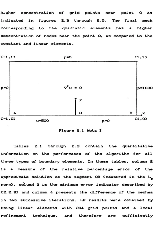
Example 2. 1 Consider Laplace's equation in a rectangular region or dimensions 2 x 1. subject to the boundary conditions described in figure 2.1 Cthe well-known Motz I problem!), where p=^r. The solution has a square root f l u x

on

singularity at point O. In general, the adaptive optimal mesh algorithm deals with the entire b o u ndary but it can equa l l y be applied to portions of the boundary which require more attention. In the present problem, the algorithm is applied to the segment AB.

higher c o n c entration of grid points near point O as indicated in figures 2 . 3 through 2. S. T h e final m esh c o r r esponding to the quadratic elements has a higher concentration of nodes near the point O. as compared to the constant an d linear elements.

C-i.iD p= 0 C l . 15

7 2u * O p-iOOO

‘ y

A O B X

»OZ>

u=500 a n O Cl .03

Figure 2.1 Motz I

Tables 2.1 thro u g h 2. 3 cont a i n the quanti tati ve i n f o r m a t i o n on the p e r f o r m a n c e of the a l g o r i t h m for all three types of b o u n d a r y elements. In these tables, c o l u m n 2 is a meas u r e of the r e l a t i v e p e r c e n t a g e error of the a p p r o x i m a t e s o l u t i o n o n th e segment O B C m e a s u r e d in the L

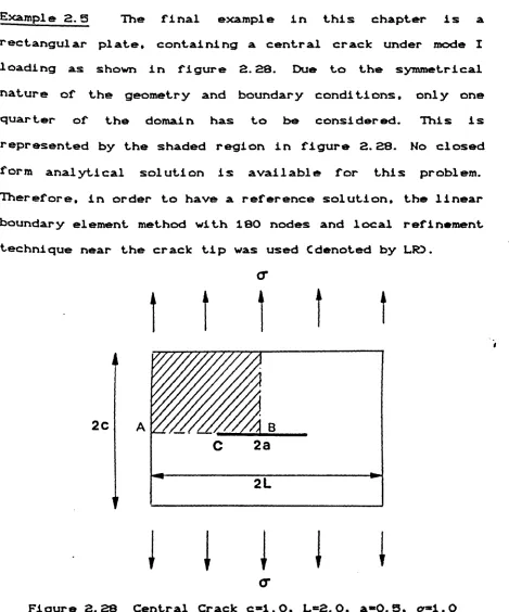
2

n o r n O , columrl 3 is the m i n i m u m error indicator d e scribed b y C 2 . 2 . Q3 and column 4 presents the d i f f e r e n c e of the meshes in two s u c c e s s i v e iterations. L R results wer e o b t a i n e d b y u sing linear elements with 2 0 4 gri d points and a local refinement technique, an d t h e r e f o r e a r e s u f f i c i e n t l y

27

accurate to represent the exact s o l ution for comparative purposes. The v a r iable u^ represents the numerical solution of the potential problem. S i n c e the approximation to the second and third derivatives is not as a c c u r a t e as that to the first derivatives near the singular point O, the co n v e rgence of a l g o r i t h m with constant element is fastest as shown in column 4 of tables 2 . 1 —2.3.

The numerical solutions on OB ar e s hown r e s p e c t i v e l y in figures 2.6. 2.7 and 2.8.

TABLE 2.1 Motz I w ith constant element

o. of iteration

juh -u 1 L>

E COBD

o E |x -x | oa

l“ h |o

O initial O. 823 Y. 0.331 E OO 0.363 E OO

1 O. 604 V. 0.663 E-Ol 0.272 E-Ol

2 O. 511 y. 0.261 E-Ol 0 .230 E —02

T ABLE 2 . 3 Motz I w i t h linear element

o.of iteration

m h LX Ju -u

rtfs'* _{E C OB3}

o E 1^.

OB -*il lu h #o

O initial O. 622 y O. 156 E O O O.131 E Ol

1 O. 401 y O. 412 E-Ol O. 281 E OO

2 O. 342 y O . 2 0 2 E-Ol O. 742 E-Ol

3 O. 298 y O . 15 2 E-Ol 0.112 E-Ol

T A B L E 2.3 M otz I w i t h quadratic element

o. of i t eration

. h L* Ju -u

»o r\tv* _{E COBD}

o E

OB "X il

I'S'lo

O initial O. 488 y O . 93 9 E-Ol 0.114 E O O

1 O. 271 y O. 31 5 E-Ol 0.190 E O O

2 O. 176 y 0 . 1 7 8 E-Ol O. 645 E-Ol

3 O. 136 y O . 121 E-Ol 0 . 128 E-Ol

29

4 --- 4--- 1--- 1--- 1--- 1--- 1--- 1--- 1--- 1--- I--- 1 --- «--- 1--- t

■4---1---1---1---— 4---•---1---1---I---1---1----1---<---1---»■

F ig u re 2.2 In it ia l M esh

H 1--- 1--- 1--- 1--- h H 1 h H 1--- 1--- h

F ig u re 2.4 T h e M esh in Ite ra tio n 3 for M o tz I ( L B E M )

B

Figure 2.5 The Mesh in Iteration 3 for Motz I (QBEM)

B

31

1000-1

INITIAL GRID

ITERATION 3

E X A C T (LR)

750-500

0

2

.4

6

1.0

X

F ig u re 2.6 T h e P o te n tia l on O B for M o t z I ( C B E M )

INITIAL GRID

ITERATION 3

EXACT(LR )

U

2

IU

u p

CO

CO

Oi

3 3

Reproduced with permission of the copyright owner. Further reproduction prohibited without permission.

Exam p l e 2. 2 The next b o u n d a r y value p r o b l e m to be solved is the well known Motz II p r o b l e m which is depicted i n figure

2. Q.

C-i.lD U_1 CO,ID P,=° Cl,ID

x -*— ►

Cl ,03 C -1 ,03

p =o

Figure 2.Q Motz II

singularities than the constant a n d linear counterparts.

Tables 2 . 4 through 2. © represent the error and conver g e n c e results on s e c t i o n OB. The c o r r esponding results on the section C D are s h o w n in tables 2 . 7 through 2.9 for all three types or elements. T h e LR results a r e o b t ained b y using linear elements wit h 2 2 4 gri d points and local refinement techniques which c a n in fact represent the exact solution nee d e d for compar a t i v e purposes. The sam e comments conce r n i n g the faster c o n v e r g e n c e of const a n t elements as in exam p l e 2.1 can be applied here.

TABLE 2 . 4 Mot z II wit h constant element

lo. of iteration

lu h Io

COBD E COBD

o T. |5\

O B

O initial 2. 79 5 V. 0 . 3 4 4 E O O O. 163 E Ol

1 2. 041 y. 0.091 E-Ol O. 152 E-Ol

2 1. 91 9 y 0 . 2 1 7 E-Ol O. 873 E —0 2

3 1. 914 y 0 . 1 7 7 E-Ol O. 991 E —03

35

TABLE 2.5 Motz II wit h linear element

o. of iteration

|u -u

lo

E COB5 o

OB l“ h |lo

O initial 1. 961 y» 0.184 E OO 0.133 E Ol

1 _{1. 481} y O. 412 E-Ol O . 554 E-Ol

2 O. 937 y O . 187 E-Ol O. 102 E —02

3 O. 872 y O. 143 E-Ol 0.355 E —03

T ABLE 2 . 6 Motz II with quadratic element

o. of iteration

a h LR a

lu ” U l o ------- 2 c O B 3

l“ h | o

E COBD

o E j ^ - x . J

O B

O initial 1. 4 3 2 y 0.965 E-Ol

i

0 .107 E Ol

1 O. 741 y. 0.270 E-Ol 0 .154 E OO

2 O. 448 y. O . 129 E-Ol 0.573 E-Ol

TABLE 2.7 Motz II w ith constant element

o.of iteration

J -U _to

vV»~rvs _{E CCDD}

o E |x

CD lu h «o

O initial 1. 826 y. O . 3 7 2 E OO 0.158 E Ol

1 O. 982 y* O . 361 E-Ol O. 433 E-Ol

2 O. 940 y. O. 211 E-Ol 0.121 E —0 2

3 O. 933 y O. 19 6 E-Ol O. 312 E —03

T ABLE 2.8 Motz II w i t h linear element

o.of iteration

■ *» LR |u -U

E C CDD

o

E |xt

CD ~X il

)

J

0

£

3

O initial 1. 421 0.134 E O O O. 146 E O O

1 O. 686 y. 0 . 3 7 7 E-Ol O. 928 E-Ol

2 O. 433 y O . 162 E-Ol O. 434 E —0 2

3 O. 3 9 9 y„ O . 13 3 E-Ol O. 988 E —0 3

37

TABLE 2.9 Motz II with quadratic element

No.of iteration

. h LX Iu “u _lo

E CCDD

o E l*t

CD -*tl |-h lo

O initial O. 920 V. O.970 E-Ol 0.113 E Ol

1 O. 491 y» O. 205 E-Ol O. 130 E OO

2 O. 290 y- O . 140 E-Ol O. 748 E-Ol

3 O. 183 y» 0.911 E-Ol O. 928 E —0 2

t D C

1--- !----1--- 1--1-t-H H <-1-,--4--- ( ■ 4 ..

-I 4- - I f---4--4-4-4+» 4 4— i f ■■ ->---1---

-A O B

Figure 2.10 The Mesh in Iteration 3 for Motz II CCBEM3

E D c

4 ■ 4 4— > ■I■t 4 4 4 4--4— 4 ■ -4---4■ ■■...

---1 4■- I---4— 1----4-4-»-4-4-4--4---4 4.... I---

-A O B

Figure 2.11 The Mesh in Iteration 3 for Motz II CLBEM3

E D C

. -4---1 4- ■.■»---4— 444-44 4--4 ■ 4■ 4...4---

-—.4 ■■> I ■ ♦— 4 44 44 4 4 4 4 4 4 4

A O ®

Figure 2.12 The Mesh in Iteration 3 for Motz II CQBEM3

39

.25-U

INITIAL GRID

ITERATION 3

EXACT LR

0

₂

₄

₆

₈

_1.0

x

F ig u re 2.13 T h e P o te n tia l on O B fo r M o tz I I ( C B E M )

.25-U

INITIAL GRID

ITERATION 3

EXACT LR

1.0

8

4

6

2

.25-U

INITIAL GRID

ITERATION 3

EXACT LR

1.0

X

F igure 2.15 T h e P o ten tial on O B for M o tz I I ( Q B E M )

INITIAL GRID

ITERATION 3

.75-U

.2

.0

.4

.6

8

1.0

X

F ig u re 2 .1 6 T h e P o te n tia l o n C D fo r M o tz I I ( C B E M )

41

INITIAL GRID

ITERATION 3

X

F ig u re 2 .1 7 T h e P o te n tia l 011 C D fo r M o tz I I ( L B E M )

1.0

INITIAL GRID

ITERATION 3

EXACT LR

.75-U

.0

.2

.4

.6

.8

1.0

2.5 Linear elasticity

The numerical results presented in the previous section s h o w that the optimal mesh algorithm i s - reliable for solving L a p l a c e ’s equation. Here we extend the algorithm originally developed b y C a r e y and Kennon CQ3 to treat the concept of asymptotic optimal mesh in the boundary element elastostatic problem. This extension has several important features. To begin with. the algorithm is simple enough to be incorporated into existing two-dimensional boundary element stress analysis codes. Furthermore, the algorithm leads to an asymptotic optimal discretization and therefore a more accurate BEM solution. In order to demonstrate the strategy, three benchmark problems are treated, one of which is a centered crack problem. All three benchmark problems involve boundaries consisting of straight line segments. The procedure is similar to that of the previous section, the major difference being in the choice of function WCxD. Both the linear and the quadratic b o u ndary elements are experimented with. Th e reason for excluding the constant elements is that t h e y are found to result in inaccurate pr edi c tions.

A word of caution is in order. Preferably, in the two-dimensional elasticity equations, the displacement variables are referred to the C x ,x D coordinate system. But for the

1 2

sake of convenience, in this chapter we ar e referring to the Cx,yD system.

43

The elasticity computer program used in this thesis is designed for two-dimensional problems and thickness variable is not requested as an input.

Example 2. 3 Here we consider a simple plane stress problem

o f t w o d i m e n s i o n a l l i n e a r e l a s t i c i t y . T h e d i m e n s i o n s *

boundary conditions and material properties are given in figure 2.19 where the imposed load is P=Py/c and P=SO. O.

2C

A

_B

Figure 2.19 The Idealized Plane Stress* Ex. 2.3* c=0.25. L*1.0, Young's modulus E=SO. O, Poisson's ratio 3.

The - exact solution to the idealized plane stress problem can eas i l y b e derived from the equilibrium equation Csee A p p endix II, 8.23 where the displacements are given b y

u^Cx,y3 P_

u^Cx.yD = C2. S. 2D

In the above expression* u^ and are the displacements in the x and y directions respectively.

The first step is to i d e n t i f y the portion Cor portions}

o f t h e b o u n d a r y w h e r e t h e m e s h i s t o b e r e d i s t r i b u t e d . I n

this particular problem* the optimal mesh a l gorithm is to be applied on the top and bo t t o m horizontal boundaries. An initial b o u ndary element mesh is chosen and shown in figure 2.20. Note that the mesh is not u n i f o r m adjacent to the corners on the two horizontal segments.

S ince an elast i c i t y problem has two dependent variables* there c a n b e different choices for the function WCxD. In this example the choice

WCsD = u CsD

2

was made, w here s is the arc length on the boundary. We also note that u cannot be chosen as WCxD beca u s e u * ' eO o n both

1 l

top and bottom horizontal boundaries. For the above choice and linear elements* the optimal mesh is determined b y C 2 . 3.ID with the function TCxD given b y

The closed f o r m analytic solution C2 . 5.2D implies that

f unction of x. Therefore, the function in C2.5.3D is constant* i . e. , an o p t i m u m u n i f o r m mesh is anticipated. N ote

TCsD - |u"CsD j2"'3 C2. S. 3D

on the top and b o t t o m boundaries* u^CsD is a quadratic

AS

that, the actual red i s t r i b u t i o n takes p lace o n l y on the top and b o t t o m horizontal boundaries. C o n v e r g e n c e to a u n i f o r m mesh is expected.

At this point the a l g o r i t h m des c r i b e d in s e c t i o n 2. 3 was applied and the results after t hree iterations are r e c orded in Table 2.10. T h e sec o n d and third columns of this table reflect the r e l a t i v e error in the two displacement components o n t h e b o t t o m b o u n d a r y m e a s u r e d in the L^—norm. Note that as the mesh is redistributed, the error is reduced raonotonically. Th e fourth co l u m n in T a b l e 2 . 1 0 describes the de viation f r o m the u n i f o r m mesh on the b o t t o m boundary. In the last row, E O D denotes the b o u n d a r y element solution on the exact optimal mesh, i.e. in C 2 . 3. ID, TC xZ> =TC xD is a k nown analytic solution.

T A B L E 2 . 1 0 Ex. 2 . 3 w i t h linear element

No. of iteration

K _ u illou r a

Ju — u h

1 2 2 »o acvs

E IXi-xfl

A B

|uh |

a i i0 |uh |a 2 *o

O initial 1. 2 0 y 3. 96 % 0 . 2 5 8 E OO

1 1.01 y 2. 5 2 y. 0 . 2 9 6 E-Ol

2 O. 3 9 y 2. 3 9 y 0. 1 5 2 E —02

3 O. 9 0 y 2. 38 y O. 11 8 E —0 3