Complete and equivalent query rewriting using views.

(1)

University of Windsor University of Windsor

Scholarship at UWindsor

Electronic Theses and Dissertations Theses, Dissertations, and Major Papers

1-1-2007

Complete and equivalent query rewriting using views.

Minghao Li

University of Windsor

Follow this and additional works at: https://scholar.uwindsor.ca/etd

Recommended Citation Recommended Citation

Li, Minghao, "Complete and equivalent query rewriting using views." (2007). Electronic Theses and Dissertations. 6993.

https://scholar.uwindsor.ca/etd/6993

(2)

C

o m p l e t e

a n d

E

q u i v a l e n t

Q

u e r y

R

e w r i t i n g

u s i n g

v i e w s

by

Minghao Li

A Thesis

submitted to the Faculty of Graduate Studies and Research

through Computer Science

in Partial Fulfillment of the Requirements for

the degree of Master of Science at the

University of Windsor

Windsor, Ontario, Canada

2007

(3)

Library and Archives Canada

Bibliotheque et Archives Canada

Published Heritage Branch

395 W ellington S treet O ttaw a ON K1A 0N4 C a n a d a

Your file Votre reference ISBN: 978-0-494-35018-8 Our file Notre reference ISBN: 978-0-494-35018-8

Direction du

Patrimoine de I'edition

395, rue W ellington O ttaw a ON K1A 0N4 C a n a d a

NOTICE:

The author has granted a non exclusive license allowing Library and Archives Canada to reproduce, publish, archive, preserve, conserve, communicate to the public by

telecommunication or on the Internet, loan, distribute and sell theses

worldwide, for commercial or non commercial purposes, in microform, paper, electronic and/or any other formats.

AVIS:

L'auteur a accorde une licence non exclusive permettant a la Bibliotheque et Archives Canada de reproduire, publier, archiver,

sauvegarder, conserver, transmettre au public par telecommunication ou par I'lnternet, preter, distribuer et vendre des theses partout dans le monde, a des fins commerciales ou autres, sur support microforme, papier, electronique et/ou autres formats.

The author retains copyright ownership and moral rights in this thesis. Neither the thesis nor substantial extracts from it may be printed or otherwise reproduced without the author's permission.

L'auteur conserve la propriete du droit d'auteur et des droits moraux qui protege cette these. Ni la these ni des extraits substantiels de celle-ci ne doivent etre imprimes ou autrement reproduits sans son autorisation.

In compliance with the Canadian Privacy Act some supporting forms may have been removed from this thesis.

While these forms may be included in the document page count,

their removal does not represent any loss of content from the

Conformement a la loi canadienne sur la protection de la vie privee, quelques formulaires secondaires ont ete enleves de cette these.

(4)

Abstract

Query rewriting using views is a technique for answering a query using a set o f views

instead of accessing the database relations directly. There are two categories of rewritings,

i.e., equivalent rewriting using materialized views applied in query optimization, and

maximally contained rewriting used in data integration. Although maximally contained

rewriting is acceptable in data integration, there are cases where an equivalent rewriting

is desired. More importantly, the maximally contained rewriting is a union of all the

contained queries, many o f which are redundant. This thesis gives an efficient algorithm

to find a complete and equivalent rewriting that is a single conjunctive query. We proved

that the algorithm is guaranteed to find all the complete and equivalent rewritings, and

that the produced rewriting is guarantee to be equivalent without additional containment

checking. We showed that our algorithm is much faster than other algorithms by

complexity analysis and experiments.

(5)

Acknowledgements

I would first like to thank my supervisor, Dr. Jianguo Lu, for his constant encouragement

and guidance. He has walked me through all the stages of my research work and thesis

writing. Without his support, the work presented in this thesis would not have become a

reality.

I would extend my appreciation to Calisto Zuzarte, Xiaoyan Qian and Wenbin Ma from

IBM Toronto Lab, for their enlightening discussion and help when I studied DB2 Query

Rewriting in IBM CAS Toronto. I would also like to thank Mr. Kenneth Cheung for his

excellent work on a preliminary version of query translating and rewriting system.

Most of all, I would like to express my deepest gratitude to my dear fiancee Ms. Juan Liu.

It is her unconditional love and support that helps me overcome all the difficulties and

finish this work eventually. My thanks would also go to my parents for their loving

considerations and great confidence in me all through these years.

Many others, too numerous to mention, provided encouragement and support as I carried

(6)

-List of Tables

Table 2-1: Bucket table for bucket algorithm ... - 22

Table 2-2: Table of view combinations... - 22

Table 3 -1: Query and views for example 3.1... -28

Table 3-2: Contained rewritings and expansions for example3.1... ... - 29

Table 3-3: Queries in example for tail containment mappings... .-31

i Table 3-4: all possible mappings in example 3.3... ...- 32

Table 3-5: Views in example 3.4... ... ... ... - 35

Table 3-6: Buckets after the first stage ... -35

Table 3-7: Buckets after applying Rule 1... ...-37

Table 3-8: Buckets after applying rule 2 ... ... ... ... - 42

Table 3-9: Matching sets for subgoals of view V I ... -4 4 Table 3-10: Constructed m appings... ...- 45

Table 4-1: The number of queries having contained or CE rewritings . .... - 53

Table 4-2: Average number of contained rewritings per query... - 55

Table 4-3: The number o f queries having CE rewritings ... - 57

Table 4-4: The total number of CE rewritings for all testing queries...-58

Table 4-5: Rewriting time for 200 queries(in m s ) ... -6 0

(10)

List of Figures

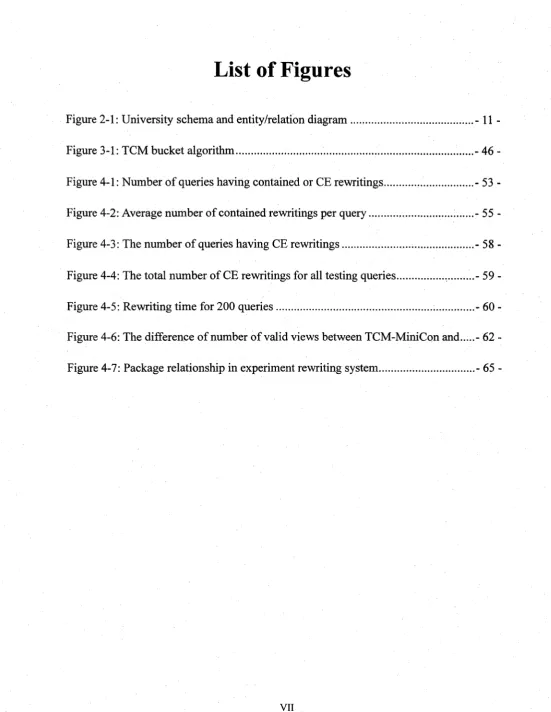
Figure 2-1: University schema and entity/relation diagram ... -11

Figure 3-1: TCM bucket algorithm... ...- 46

Figure 4-1: Number o f queries having contained or CE rewritings ...- 53

Figure 4-2: Average number of contained rewritings per query ... ...-55

Figure 4-3 : The number of queries having CE rewritings... ... ... - 58

Figure 4-4: The total number of CE rewritings for all testing queries... ... - 59

Figure 4-5: Rewriting time for 200 queries ... ...- 60

Figure 4-6: The difference o f number o f valid views between TCM-MiniCon and... 62

(11)

Chapter 1 Introduction

1.1 Application Background

Query rewriting using views is also known as answering query using views [1] or query

folding [2]. Informally speaking, the problem can be described as following: given a

i query on a database schema, and a set of views over the same schema, how can the query

be rewritten so that it partially or completely refers to the set of views? Query rewriting

plays a very important role in many database management applications, such as query

optimization [3, 4], data integration [5, 6, 7, 8], and data warehouse [9, 10, 11].

In query optimization, some views are created to perform the frequently executed query

operations, and the results of these views are stored in disk for future uses. These views

are called materialized views. Given a query posed over database relations, if it can be

answered using materialized views, then the evaluation process of this query will become

more efficient, because some computations are pre-performed by the materialized views.

Therefore, from the query optimization point of view, query rewriting is to generate

logical plan that is equivalent to the original query using materialized views.

In the context of data integration, query rewriting using views is also unavoidably

(12)

systems, such as Information Manifold [5] and Infomaster [12], provide a uniform query

interface to a number of heterogeneous data sources. In order to do so, the data

integration system first defines a global schema according to a particular application, and

then describes all data sources as views over the global schema. Users pose queries over

the global schema as well. Global schema, however, is a set of virtual relations, which

means there is no actual data stored in them. In order to answer those queries, the system

has to find rewritings of the queries that only refer to data source descriptions (views).

The rewriting result might be a union of several queries that are contained in the original

query.

This thesis focuses on the discussion of query rewriting algorithms for data integration

applications. Thus in the next section, we will talk about data integration architecture in

more detail.

1.2 Data Integration

1.2.1 Introduction

Along with the booming o f World Wide Web, there is tons of information on the Internet.

Apart from the Web, there is also a large number of public databases and many other

(13)

can we make efficient use of all those information? Data integration system is one of the

solutions to this problem.

Data integration system provides uniform access to various distributed heterogeneous

information sources. The information sources can include traditional database systems,

structured data like XML files, or even semi-structured data like information in HTML

pages. Data integration system frees the users from finding information from many

t different sources and then manually combining them together. Taking advantages of data

integration architecture, users are able to pose queries against a uniform schema, without

knowing the type of data sources that is used behind.

In previous researches, several information integration systems have been proposed.

• Information manifold, a project of AT&T Lab [5].

• TSIMMIS, a cooperative project between Stanford University and IBM [6].

• Infomaster, a practical integration system from Stanford University [12].

• SIMS, a service and information management system for decision support [13].

1.2.2 Data Source Modeling

Data integration system is also known as mediator system. The two approaches to define

(14)

1. Global-As-View (GAV) approach defines the mediator schema as views in terms of

the schema of information sources. The mediator schema is considered as a set of

query patterns. A query is defined in terms of mediator schema. A query can be

answered by the mediator if it matches one of those patterns, otherwise it cannot be

handled. When a data source is added into or removed from the mediator, the

mediator schema has to be reformulated. Some known data integration systems are

based on GAV approach, for example, TSIMMIS, a cooperative project between

Stanford University and IBM [6], TSIMMIS uses GAV approach although it adopts

a different rule language.

2. Local-As-View (LAV) approach is the opposite of GAV. The mediator schema in

LAV is a global virtual schema designed according to the need of specific

application. It is called virtual schema because there is no data actually stored in the

mediator schema. Both user queries and source descriptions are defined in terms of

the global schema.. In order to answer a query, the system first rewrites the query

using source description views, and then retrieves the best result from the rewritings.

Since the virtual mediator schema contains no data, the rewritten query must only

refer to data descriptions (views). Because some data sources might be incomplete,

the system allows a rewritten query not equivalent to the original query, but to be

(15)

Adding or deleting an information source is just creating or removing a source

descriptor. Therefore, the data integration system based on LAV approach has

excellent extendibility and is suitable for Internet based applications. Information

Manifold system from AT&T Lab [5] and Infomaster system from Stanford

University [12] are two famous data integration systems that use LAV approach.

In these two systems, query rewriting plays an essential role. In the following

sections, we will introduce some existing query rewriting algorithms used in data

integration applications.

1.3 Query Rewriting Using Views

Query rewriting using views is a technique that offers a way to answer a query referring

to pre-defmed views instead of database relations. According to different criteria, query

rewritings can be categorized into:

1. Complete Rewriting vs. Partial Rewriting

• Complete Rewriting is a rewriting of query that only refers to views.

• Partial Rewriting is a rewriting of query that refers to both views and database

(16)

2. Equivalent Rewriting vs. Maximally Contained Rewriting

• Equivalent Rewriting is a rewriting having the same answer set as the original

query.

• Contained rewriting is a rewriting whose answer set is contained by the answer

set of the original query.

• Maximally contained rewriting is a contained rewriting whose answer set

contains the answer set of any other contained rewriting of the query.

Different applications require different type of query rewritings. Query optimization

application looks for an equivalent rewriting that has the shortest evaluation time, while

data integration application needs a rewriting that only refers to views and has the same

answering set as the original query. Therefore, complete and equivalent rewriting, also

known as CE rewriting is the best solution for data integration application. However,

some queries might not have equivalent rewriting based on all available views, and then

complete maximally contained rewriting can work as an alternative solution.

Many algorithms have been proposed to solve the query rewriting problem for data

integration applications. These algorithms generally fall into two classes: bucket-based

algorithm and inverse rule-based algorithm. The primary bucket algorithm was first

proposed by A.Y. Levy in [5]. More recently, some other bucket-based algorithms, such

(17)

CoreCover algorithm [16] were developed to improve the performance o f primary bucket

algorithm.

The idea of inverse rule was first proposed by X. Qian in [2], and presently the inverse

rule algorithm was formally discussed in [17]. We are going to review these algorithms

in section 2.3.

1.4 Thesis motivation and contribution

Existing complete query rewriting algorithms [5] [14] [15] [16] are designed to produce

complete maximally contained rewritings. The result of those algorithms is a union of all

complete contained rewritings that can be found. In application where there is a large

number of views available for query rewriting, there might exist a single conjunctive

query that is equivalent to the original query. This equivalent rewriting itself is sufficient

to answer the query. However, existing complete query algorithms include all the other

contained conjunctive queries into the result, which in fact are redundant and make the

evaluation of the rewriting inefficient.

In order to find the complete and equivalent conjunctive rewriting, we propose a TCM

(Tail Containment Mapping) Bucket algorithm that expands the bucket algorithm to

(18)

inappropriate views from being added to the buckets generated in the first stage of the

bucket algorithm, so that the rewritings produced in the combination stage are

automatically CE rewritings without any extra containment checking.

In the experiments o f this thesis, we implement MiniCon algorithm, an advanced bucket

based algorithm, with our TCM checking rules and compare this combination with some

other algorithms. All testing data we use in our experiments, containing hundreds of

relations, views and queries, are extracted from real e-commerce projects, rather than

generated by ourselves.

1.5 Thesis overview

The main body o f this thesis is organized as follows. Chapter 2 introduces the relevant

notations, gives the formal definition of the query rewriting problem and some important

concepts, and briefly goes over two previous query rewriting algorithms in the last

section. In chapter 3, we first discuss the motivation and benefit of answering query

using complete equivalent rewriting, and then we present our TCM bucket algorithm.

Chapter 4 provides the results and analyses of the experiments that we conduct. Chapter

(19)

Chapter 2 Overview of Query Rewriting Using Views

In this chapter, we will first introduce some concepts that are related to query rewriting

using views and are used throughout this thesis. Secondly, we will describe some

different kinds of query rewritings surveyed in [1]. And at last, we will discuss some

related works that have been already done under this topic.

2.1 Query Language

All the queries and views discussed in this thesis are SPJ queries, whose relational

algebra expressions only contain project, select and join operations. We also assume that

no queries contain redundant subgoal, and that neither query nor view contains

comparison predicates.

We use Datalog to define all the queries and views in this paper. Datalog [18] is a

powerful query language that is widely used to express queries and views in [16, 15, 14,

19]. Using Datalog expression, a SPJ query Q can be conveyed to a rule in the following

form:

(20)

where Q and n , • • •, rn are predicate names, and X, Xi, • • •, Xn are tuples of variables

or constants. Q( X) is the head of query, denoted by H(Q). Variables in X are called

distinguished variables or head variables. The variables in X i, • • • , X„ but not in X are

called existential variables. To be safe, distinguished variables must also appear in

subgoals of relations or views. ri( Xi), • • • , rn( Xn) are called source subgoals, which

refer to database relations or views. And we use Subgoal(Q) to denote all source relations

of a query Q.

In a datalog clause, we always assume that the ith variable of a subgoal r(X) refers to the

th

i attribute o f the relation table that r(X) refers to. And the fact that the same variable

appears in two source subgoals implicates that there is a join predicate on this variable

between the two relations or views referred by these two subgoals. Such variables are

called join variables. A Datalog clause may also include subgoals of arithmetic

comparison predicates, such as <, =, >• These subgoals are called comparison subgoals.

Variables in a comparison subgoal must also appear in subgoals of relations or views.

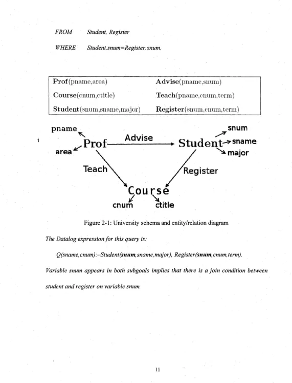
Example 2.1 Here we give an example o f Datalog notation based on a university

schema as in Figure 2-1 [1J. We will use this schema throughout this thesis. Based

on this schema, suppose there is a query that asks fo r the name o f a student and the

course this student registered. The SQL expression fo r this query is as follows:

(21)

FROM Student, Register

WHERE Student. snum= Register, snum.

P r o f

(pname, area)

A dvise(pna

me .snum)

'Course

(cnum, ctitle)

S tu dent

(simiiijSiianiejiiajo

Teachfpnau

f)

R eg iste r

(si

ie, cnum, term)

turn.cnum. term)'

pname

snum

Advise

S tu d e n t^ sname

major

Register

Course

/

V

cnum

ctitle

Figure 2-1: University schema and entity/relation diagram

The Datalog expression fo r this query is:

Q(sname, cnum):-Student (snum, sname, major), Register (snum, cnum, term).

Variable snum appears in both subgoals implies that there is a jo in condition between

(22)

2.2 Query Rewriting

2.2.1 Query Containment and Equivalence

The problem of conjunctive query containment was first studied in [20]. Query

containment is used to decide the containing relationship between two queries, and is

important to check the correctness o f a query rewriting. The formal definition of query

containment and equivalence is as below [1].

Definition 2.1 (Query containment and equivalence)

A query Qi is sa id to be contained in another query Q2, denoted a s Qj c : Q2, i f f o r any

database D, the set o f tuples com puted f o r Qi is a subset o f those com puted f o r Q2, i.e.,

Qi(D) cr Q2(D). The tw o queries are sa id to be equivalent, den oted as Qi = Q2, i f Qi cr

Q2 and Q2c " Qi.

2.2.2 Containment Mapping

Generally speaking, whether a query Qi is contained in query Q2 is undecidable. For

conjunctive queries that are considered in this thesis, the containment relationship is

decidable [21]. Containment mapping [20] provides a method to decide containment

relationship between conjunctive queries.

(23)

It maps a variable in ith position of a source subgoal in query Qi to a variable in ith

position of a subgoal referring to the same relation in query Q2. A formal definition of

containment mapping is given below [18]:

Definition 2.2 (Containment Mapping)

Given two queries Qi and Q2 over database schema S, and a mapping cp from variables

o f Q2 to variables o f Qi. Mapping cp is a containment mapping from Q2 to QI, i f

1. The head o f Q2 maps to the head o f Qi; and

2. Every subgoal o f Q2 is mapped to a subgoal o f Qi.

Intuitively, a containment mapping from Q2to Qiguarantees that all join relationships in

query Q2 are retained in query Qj. In addition, query Q; may have more subgoals than

query Q2.Thus, comparing to Q2,query Qi has same or even stricter conditions to select

tuples. There is a well-known and important conclusion based on containment mapping

as below [18].

Theorem 2.1 Given conjunctive queries Qi and Q2, Qi c; C hif and only if there is a

containment mapping from Q2 to Qi.

Example 2.2 Suppose we have three queries as below:

Q i(pnal,cnul,snul):-Teach(pnal,cnul,terl), R egister(snul,cnul,terl)

Student (snul,snal,m ajl)

(24)

Q3(pnaS, cnu3, sna3):-Teach(pna3, cnu3, ter3), Register(snu3, cnu3, ter3)

We can form a mapping (p2ifrom Q2 to Qi as following:

<P2P {pna2 -^pnal, cnu2 ->cnul, ter2 ->terl, snu2 ->snul ter2 ’-U teri’}

(P2 1 satisfies the conditions o f containment mapping, so QI is contained by Q2. For query

Q3, the only possible mapping cp 3 1 we can construct from Q3 to Qj is shown below.

<P3d {pna3 ~>pnal, cnu3 ->cnul, ter3 ->terl, snu3 ->snul ter3 ->terl ’}

However, it is not a containment mapping because variable ter3 o f Q3 is mapped to two

different variables terl and terl ’ o f Qj. As a result, Qi is not contained by Q3.

Theorem 2.1 provides a basic way to check whether a conjunctive query Qi contains

another query Q2. Finding containment mapping from Qi to Q2 is an NP-complete

problem [20]. In the worst case, its time complexity is 0(m n), where n is the number of

subgoals in Qi and m is the number of subgoals in Q2. In practice, the size of queries or

views is usually not large; hence, the execution time for containment checking is

acceptable. More important, the performance of an algorithm could be significantly

improved if the use of containment checking is avoided or reduced.

2.2.3 Query Rewriting Using Views

The problem of query rewriting using views, a.k.a. answering query using views, is about

(25)

instead of accessing the database relations. The formal definitions of two kinds of query

rewritings are shown below.

Definition 2.3 (Equivalent Rewriting) [1]

Given a query Q referring to database relations o f a schema, and a set o f views V =

Vi, ■ ■ ■, Vm over the same schema, the query Q ’ is an equivalent rewriting o f Q using V

i f

• Q ’ refers to one or more views in V; and

• Q ’ is equivalent to Q.

Definition 2.4 (Maximally-Contained Rewriting) [1]

Given a query Q referring to database relations o f a schema, and a set o f views V =

Vj, ■ ■ -, Vm over the same schema, Q ’ is a rewriting o f Q using views from V, then

1) Q ’ is a contained rewriting o f Q, i f Q ' c:Q.

2) Q ’ is a maximally-contained rewriting o f Q if:

• Q ’ c:Q; and

• There is no another rewriting Q ” o f Q using the same query language, such

that Q ’ c Q ” c Q , i.e., fo r any database D, Q ’(D) cr Q ”(D) cr Q(D).

Definition 2.5 (Complete and Equivalent Rewriting) [1]

Given a query Q referring to database relations o f a schema, and a set o f views V =

V i , " - ; V m over the same schema, Q ’ is a rewriting o f Q using views from V, then

(26)

2) Q ’ is a complete and equivalent rewriting o f Q if:

• Q ’ is complete rewriting; and

• G’« 0 .

In this thesis, we abbreviate the complete and equivalent rewiring to CE rewriting.

Here are some examples of different types of query rewritings.

Example 2.3 Suppose that we have a query over the schema defined above which

asks fo r student names who are taught by professors in “Database ” area in winter

term.

Q(sname):—Register(sname, cnum, term), Teach(pname, cnum, term, year),

P ro f (pname, area), area= “Database ”, term=“w in ”.

Besides the database relations, we have two views Vj and V% Vj shows the professors in

Database area and the courses they teach. V2 shows the registration information in

winter term.

Vj (pname, cnum):-Prof(pname, area), Teach(pname, cnum, term),

area= “Database

V2 (sname, cnum):-Register (sname, cnum, term), term=“w in ”.

There are three rewritings o f query Q using Vj and V2 shown below. We can see both Q )

and Q '2 are partial rewritings, while Q ’3 is a complete rewriting o f Q.

Q ’i(sname):-V](pname,cnum), Register (sname, cnum, term), term =“w in ”.

(27)

Prof(pname,area), area= ’’Database

Q ’3(sname):-Vi(pname,cnum),V2(sname,cnum).

Query rewriting is used in various database applications. Different applications require

different kinds of query rewritings. For the purpose of query optimization, equivalent

rewriting is required, but both complete and partial rewritings are acceptable. While in

data integration applications, the rewriting must be complete rewriting, because data

* relations in this case are virtual relations and actual data sources are described as views.

When equivalent rewriting cannot be approached, maximally-contained rewriting is

accepted then. In this thesis, we only discuss the problem of finding complete rewriting.

2.2.4 Query Expansion

For a query Q over a database schema referring to not only relations but also views, the

expansion of Q is a query Qx constructed by substituting the views in the body of Q with

their definitions and renaming the variables to maintain the equivalence with the original

query Q.

Suppose the original query is as below:

Q(X):- ri(X i),. ., rn(Xn), V (Y).

(28)

V (Z ):-p1(Z1) , . ; . , p m(Zm).

then the expansion o f Q is o f the form:

Q x ( X ) : -nCXO,. . . , rn(Xn), pK V O ,. . . , pm(Vm). Q x is created in two steps:

1. Replace the subgoal V(Y) in Q with the body o f the definition of view V.

2. Rename all variables from V definition, Z \ ,... ,Zm, using the following rules:

(a) If variable Zj is a distinguished variable o f V, i.e., z; e Z, rename Zj as a

corresponding variable in Y from the original query.

(b) If variable z; is an existential variable of V, i.e., z* gZ, rename Z; as a new

variable of Q which is not in Xi U . . . U Xn.

Example 2.4 Consider the following query and views:

Q(pname, cnum,sname):-V](pname,area,snum), V2(pname,area, cnum),

Student (snum,sname,majo).

Vi(pnal,arel,snul) Advise(pnal,snul), Prof(pnal,arel.)

V2(pna2,are2,cnu2) Prof(pna2,are2), Teach(pna2,cnu2,ter2).

The expansion o f Q is as below:

Qx(pname, cnum, sname):—Advise(pname,snum), Prof(pname,area),

Prof(pname,area), Teach(pname,cnum,ter2)

(29)

2.2.5 Rewriting Containment Verification

Given a query Q on a database schema S, and a rewriting Q ’ o f Q referring to some

views over the same schema, it is not applicable to compare Q and Q ’ directly, but taking

advantage of Q ’x , it can be decided whether Q ’ is contained or equivalent to Q .

The rewriting Q ’ referring to Y is computed using view instance d. While in Q ’x , all

subgoals referring to views are substituted by the definitions o f these views, so that Q ’eXp

refers to database relations. Based on our assumption that the instance of any view

contains all tuples that satisfy its definition, we can infer that Q ’ and Q ’x yield the same

set of resulting tuples, i.e., Q ’ = Q ’x.

For a rewriting Q ’ o f query Q, both Q ’x and Q refer to schema S, therefore according to

Theorem 2.1, it can be decided whether Q ’x is contained or equivalent to Q by finding

containment mapping between Q and Q’x. Furthermore, it can be inferred whether Q ’ is

contained or equivalent to Q using corollary 2.1.

Corollary 2.1 Given a database schema S, a set o f views V is defined on S. Suppose Q is

a conjunctive query on S, and Q ’ is a rewriting o f Q referring to V.

1) Q ’ c Q i f f Q f c z Q .

(30)

2.3 Previous Algorithms for Query Rewriting

Two types of rewriting algorithms have been proposed for data integration applications

in previous researches: bucket based algorithm and inverse rule based algorithm. The

primary bucket algorithm was first proposed by paper [5] for Information Manifold

system. In the later research, several improved version of bucket algorithm were

developed, such as MiniCon algorithm [14], shared variable bucket algorithm (SVB) [15]

and CoreCover algorithm [16]. The basic idea about inverse rule was proposed by paper

[2], and was then developed into the inverse rule algorithm in [17]. Other inverse rule

based algorithms were proposed in [22], [19]. Both bucket based algorithms and inverse

rule based algorithms aim to find maximally contained rewriting, so that output o f these

algorithms are a union of all contained rewritings that can be found.

Before continuing the thesis, it may be necessary to introduce the bucket algorithm in

more detail.

Bucket Algorithm

The input of bucket algorithm is a conjunctive query Q referring to database relations and

a set of views V: Vi, • • • , Vn. Both the query Q and view Vi are non-recursive SPJ

(project-select-join) queries. The output of bucket algorithm is a union of conjunctive

(31)

With the input Q and V, bucket algorithm proceeds in following two steps.

1. bucket constructing

For each source subgoal r e subgoal(Q), create a bucket, and put the views V; e V ,

which can satisfy the following condition, into the bucket o f subgoal r.

• View Vi has a subgoal ryi, representing the same relation to r, and there exists a

partial containment mapping \|/ from r to rv i.

When a view is added to a bucket, the view variables in the domain of \jr are renamed

as the corresponding variables of Q, while other variables are renamed as new

variables (primed).

2. making Combination and containment checking

First, make a Cartesian product within all buckets, and for each tuple of the result of

Cartesian product, create a conjunct query Q ’ by joining all elements in the tuple.

Then proceed a containment checking to decide if Q ’ c Q. If so, add Q ’ to the output

union.

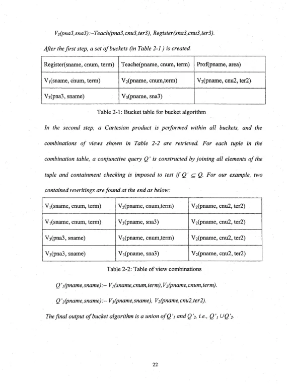
Example 2.5 Suppose we have the query and views as following.

Q(pname,sname).-Register(sname, cnum, term), Teach(pname, cnum,term),

Prof(pname,area).

Vfsnal, cnul, terl) .-Register(snal, cnul, terl), Course(cnul, ctil).

(32)

V3(pna3, sna3):-Teach(pna3, cnu3, ter3), Register(sna3, cnu3, ter3).

After the first step, a set o f buckets (in Table 2-1) is created.

Register(sname, cnum, term) Teache(pname, cnum, term) Prof(pname, area)

Vi(sname, cnum, term) V2(pname, cnum,term) V2(pname, cnu2, ter2)

V3(pna3, sname) V3(pname, sna3)

Table 2-1: Bucket table for bucket algorithm

In the second step, a Cartesian product is performed within all buckets, and the

combinations o f views shown in Table 2-2 are retrieved. For each tuple in the

combination table, a conjunctive query Q ’ is constructed by joining all elements o f the

tuple and containment checking is imposed to test i f Q ’ cr Q. For our example, two

contained rewritings are fo u nd at the end as below:

Vi (sname, cnum, term) V2(pname, cnum,term) V2(pname, cnu2, ter2)

Vi (sname, cnum, term) V3(pname, sna3) V2(pname, cnu2, ter2)

V3(pna3, sname) V2(pname, cnum,term) V2(pname, cnu2, ter2)

V3(pna3, sname) V3(pname, sna3) V2(pname, cnu2, ter2)

Table 2-2: Table of view combinations

Q ’](pname,sname)V](sname,cnum, term), V2(pname,cnum,term).

Q jfpnam e,snam e):-V3(pname,sname), V2(pname,cnu2,ter2).

(33)

Chapter 3 Finding Complete and Equivalent Rewriting

In the last chapter, we have introduced some algorithms of answering query using views.

The objective of those algorithms is to find maximally contained rewriting. In this

chapter, we will present our TCM (Tail Containment Mapping) Bucket algorithm, which

is designed to find equivalent and complete rewritings for a conjunctive query. We will

first explain the motivation of our research in section 3.1. Then, we will discuss two

solutions for finding complete and equivalent (CE) rewritings. In section 3.3, we will

propose our TCM Bucket algorithm, and the analysis of its time complexity will be given

in the last section.

3.1 Motivation

In the context of data integration, most of query rewriting algorithms [5][14] [15] [16]

are designed to produce maximally contained rewriting. The output of those algorithms is

a union of all contained rewritings they can find. We denote such maximally contained

rewriting as Q ’m, Q ’m = Q ’ i U , . . . , U Q ’n, where Q ’i, 1 < i < n, is a conjunctive

(34)

However, among all those contained rewritings Q ’ i, . . . , Q ’n, there might be an

equivalent single conjunctive rewriting, say it is Q ’i, Q ’j = Q , and i is in {1, ..., n}.

Obviously, answering Q using Q ’i will be much more efficient than using Q ’m- Since Q ’i

is already equivalent to Q , there is no need to evaluate all other contained rewritings in

Q ’ l, • • • ,Q ’n •

In application where a large number of views are available for query rewriting, the

number of contained rewritings for a query could also be very large. Among those

contained rewritings, there usually exist CE rewritings. For example, in our experiment

in section 4.2.1, when the number of views is 450, 158 queries have 3273 contained

rewritings in total. On average, a query Q has 20 contained rewritings. 116 out of these

158(73%) queries have CE rewritings. Suppose a query Q has 20 contained rewritings,

and one of those rewritings, say Q ’e is equivalent to Q , then using Q ’e instead of Q ’m to

answer query Q will have following significant benefits:

• Save the time on generating other 19 contained rewritings.

• Avoid evaluating all other 19 contained rewritings.

• Save the time on making a union of the results of all rewritings.

Suppose it takes the same time to evaluate every single conjunctive contained rewriting,

then using Q ’e to answer Q will be at least 20 times faster than using Q ’M .

(35)

rewritings for data integration applications. We have explored two approaches to find CE

rewriting. One is expanding equivalent rewriting algorithms, and the other one is

utilizing complete rewriting algorithms.

3.2 Expanding equivalent rewriting algorithms

Equivalent query rewriting algorithms [23, 24] are designed for the purpose of query

♦ optimization. The result of those algorithms are required to be equivalent rewritings, but

not necessary to be complete.

In an equivalent rewriting algorithm, the rewriting is achieved by a sequence of

substitutions. Each substitution replaces one or more subgoals o f the original query with

that of the given views. In order to obtain an equivalent rewriting in the end, the

algorithm guarantees the result of each substitution to be equivalent to the original query.

In general, it requires that every substitution is a safe substitution [23], which means all

subgoals and predicates o f the view must be able to be mapped to their counterparts of

the original query.

Due to the sequential application of the substitutions and the strict restriction on safe

substitution, in certain cases such algorithm cannot find any complete rewriting even if

(36)

and two views refer to R. In this case, one view is used and the relation R is removed,

hence the second view can never be used and some possible CE rewritings may be

missed.

Example 3.1 Given one query Q and two views V/ and V2 as below:

Q(a, d) :-A (a, b), B(b, c), C(c, d).

Vj(a, b, c) :-A (a, b), B(b, c).

V2(b, c, d) B(b, c), C(c, d).

Obviously, Vi can substitute subgoals A and B in Q, and V2 can substitute subgoals B

and C in Q. Because both two substitutions are safe substitutions, after the first iteration,

an equivalent rewriting algorithm will generate two partial equivalent rewritings:

Q’i(a, d) V,(a, b, c), C(c, d).

Q’2( a ,d ) :- A ( a ,b ) ,V2(b ,c ,d ).

Nevertheless, in the next iteration, we find out that subgoal C in Q ’i cannot be safe

substituted by V2. Because subgoal B has been replaced by Vi already, B in V2 is not

able to be mapped to any subgoal in Q’i. Likewise, situation exists between Q2and Vi.

As a result, the algorithm stops, and Q’i and Q’ 2 are the final result. However, the

algorithm misses two CE rewritings:

Q’3( a ,d ) : - V1( a ,b ,c ’) ,V2(b ,c,d ).

(37)

In order to make use of equivalent query rewriting algorithms to find CE rewritings, we

have to adjust the query to be rewritten, in every iteration of substitution, by adding some

extra subgoals and predicates, so that we can continuously conduct safe substitutions

until all source subgoals in the query are replaced by views. However, adding extra

subgoals will add unnecessary overhead, and make the algorithm very complicated.

Equivalent query rewriting algorithm, therefore, is not a proper start point for CE

4 . .

rewritings.

3.3 Expanding Complete Rewriting Algorithms

Complete rewriting algorithms are designed for data integration applications.

Accordingly, the result of this kind of algorithms must be complete rewriting. There are

two major types of complete rewriting algorithms, bucket based algorithm [5, 14, 15] and

inverse rule based algorithm [2, 17]. Complete rewriting algorithms can always find

maximally contained rewritings. It implies that if there exist equivalent rewritings of the

original query based on the given views, these algorithms can find at least one of them.

The only problem is that such algorithm does not generate any single conjunctive query

as its result; instead, it produces a union of all contained conjunctive queries.

(38)

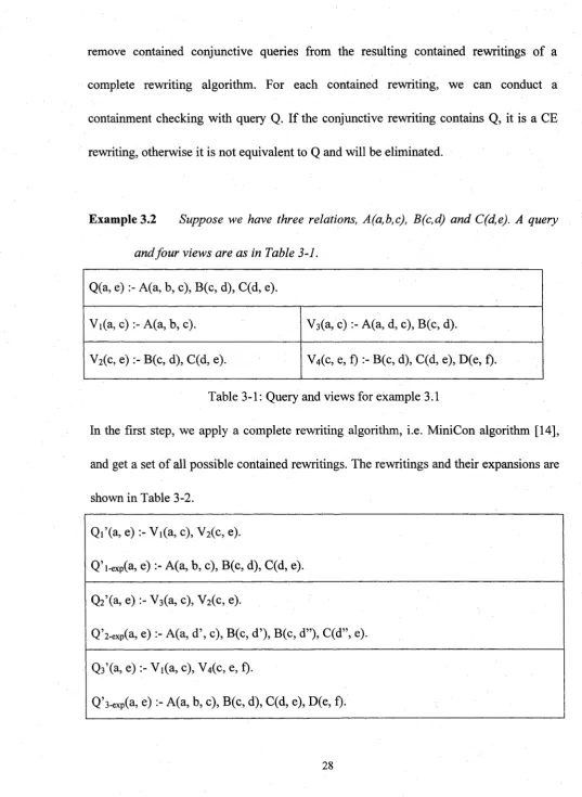
remove contained conjunctive queries from the resulting contained rewritings of a

complete rewriting algorithm. For each contained rewriting, we can conduct a

containment checking with query Q. If the conjunctive rewriting contains Q, it is a CE

rewriting, otherwise it is not equivalent to Q and will be eliminated.

Example 3.2 Suppose we have three relations, A(a,b,c), B(c,d) and C(d,e). A query

and four views are as in Table 3-1.

Q(a, e ) :- A(a, b, c), B(c, d), C(d, e).

Vi(a, c ) : - A(a, b, c). V3(a, c ) :- A(a, d, c), B(c, d).

V2(c ,e ):-B (c ,d ),C (d ,e ). V4(c, e, f) :- B(c, d), C(d, e), D(e, f).

Table 3-1: Query and views for example 3.1

In the first step, we apply a complete rewriting algorithm, i.e. MiniCon algorithm [14],

and get a set of all possible contained rewritings. The rewritings and their expansions are

shown in Table 3-2.

Q i’(a,e) :-V !(a,c), V2(c, e).

Q ’ i-exp(a, e) :- A ( a , b, c), B(c, d), C(d, e).

Q2’(a, e) :- V3(a, c), V2(c, e).

Q ’2-exp(a, e) :- A ( a , d \ c), B(c, d ’), B(c, d”), C(d”, e).

Q3’(a, e ) : - V1(a ,c ),V4(c, e, f).

(39)

Q4’(a, e) V3(a, c), V4(c, e, f).

Q’4-exP(a, e ) A ( a , d’, c), B(c, d’), B(c, d”), C(d”, e), D(e, f).

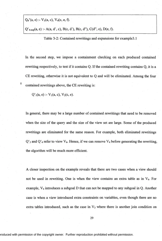
Table 3-2: Contained rewritings and expansions for example3.1

In the second step, we impose a containment checking on each produced contained

rewriting respectively, to test if it contains Q. If the contained rewriting contains Q, it is a

CE rewriting, otherwise it is not equivalent to Q and will be eliminated. Among the four

contained rewritings above, the CE rewriting is:

Q’](a,e) : - Vi(a, c), V2(c, e).

In general, there may be a large number of contained rewritings that need to be removed

when the size of the query and the size of the view set are large. Some of the produced

rewritings are eliminated for the same reason. For example, both eliminated rewritings

Q’ 3 and Q’ 4 refer to view V4. Hence, if we can remove V4 before generating the rewriting,

the algorithm will be much more efficient.

A closer inspection on the example reveals that there are two cases when a view should

not be used in rewriting. One is when the view contains an extra table as in V4. For

example, V4 introduces a subgoal D that can not be mapped to any subgoal in Q. Another

case is when a view introduced extra constraints on variables, even though there are no

(40)

the second attributes o f A and B. In this case, variable d’ in expansions of Q’ 2 and Q’4,

which is introduced by V 3 , can not be mapped to any variable in Q. Hence, Q’ 2 and Q’ 4

are not equivalent to Q.

Based on the observations above, we can see that view V 3 and V4 should not be used to

generate CE rewriting of Q. Therefore, we should eliminate V 3 and V4 before rewritings

are constructed, hence prevent non-equivalent rewriting Q ’2, Q’ 3 and Q’ 4 from being

generated, and avoid afterward containment checking.

3.4 TCM Bucket Algorithm

We now propose an algorithm that expands the bucket algorithm, a complete rewriting

algorithm, to generate CE rewriting, which is much efficient than the naive approach in

section 2.3. The main idea is to prevent inappropriate views from being added to the

buckets in the first stage of the bucket algorithm, so that the rewritings produced in the

combination stage are automatically CE rewriting without any extra containment

(41)

3.4.1 Definitions

Before going into the detail of TCM bucket algorithm, we first introduce some

definitions and terms used in the algorithm.

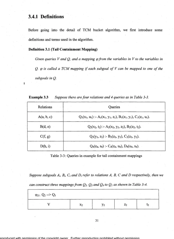
Definition 3.1 (Tail Containment Mapping)

Given queries V and Q, and a mapping (p from the variables in V to the variables in

Q. cp is called a TCM mapping i f each subgoal o f V can be mapped to one o f the

subgoals in Q.

Example 3.3 Suppose there are four relations and 4 queries as in Table 3-3.

Relations Queries

A(a, b, c) Q i(xb ui) Ai(xb yi, zO, Bi(zi, yi), Ci(zi, ui).

B(d, e) Q2(x2, t2) A 2(x2, y2, z2), B2(z2, t2).

C(f, g ) QaCys, z3) B3(z3, y3), C3(z3, y3).

D (h,i) Q4(z4, s 4) C4(Z4, m), D4(u4, s 4).

Table 3-3: Queries in example for tail containment mappings

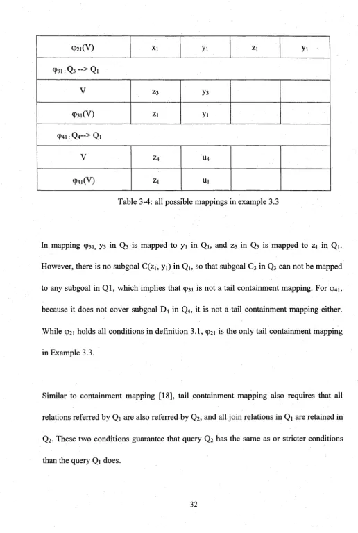
Suppose subgoals A„ Bi:C, and Dt refer to relations A, B, C and D respectively, then we

can construct three mappings from Q2, Q3 and Q4 to Qj as shown in Table 3-4.

921 : Q2 Ql

(42)

9 2 i ( V ) X i _{y i} Z i _{y i} <P31 :Q 3 “ > Ql

V Z 3 _Y3

9 3 i ( V ) Z i _{y i}

941 : Q 4 ” > Ql

V z4 u4

q>4i(V) Z i U i

Table 3-4: all possible mappings in example 3.3

In mapping (p^ y3 in Q3 is mapped to yi in Qi, and z3 in Q3 is mapped to z\ in Qi.

However, there is no subgoal C(zi, yi) in Qi, so that subgoal C3 in Q3 can not be mapped

to any subgoal in Q I, which implies that cp3i is not a tail containment mapping. For cp4i,

because it does not cover subgoal D4 in Q4, it is not a tail containment mapping either.

While 9 2 1 holds all conditions in definition 3.1, 9 2 1 is the only tail containment mapping

in Example 3.3.

Similar to containment mapping [18], tail containment mapping also requires that all

relations referred by Qi are also referred by Q2, and all join relations in Qi are retained in

Q2. These two conditions guarantee that query Q2 has the same as or stricter conditions

(43)

The difference between tail containment mapping and containment mapping is that tail

containment mapping does not require that all head variables of Q2 can be mapped to

head variables of Qi. Intuitively, a tail containment mapping from Q2 to Qi represents

that without considering projection to head variables, tuples that satisfy Qi also satisfy

q2.

f In order to verify TCM mapping, we first introduce some definitions and theorems.

Definition 3.2 (Variable Range)

Given a query Q, fo r any variable x e Q, the range o f x in Q, denoted by R(x, Q), is

the set o f relation attributes to which x refers.

For example, there are two relations A(a,b,c) and B(d,e), and a query Q(z) A(x,y,z),

B(z,u). Then the range of variable x in Q is {A.a}, i.e. R(x,Q) = {A.a}, and the range of z

in Q is {A.c,B.d}, i.e. R (y,Q )= {A.c,B.d}.

The range o f variable x in query Q reflects the specific join relationship in query Q. If

R(x,Q) contains only one attribute, it means there is no join on that attribute. If R(x, Q)

has more than one attributes, it implicates that in query Q, all those attributes are joined

(44)

Definition 3.3 Given subgoal S j( x i,.., x j from query Qi, and S2(yi,. . .,yr) from query Q2,

Si can be mapped to S2, i f

1. Si and S2 refer to the same database relation, and

2. The r a n g e o f any variable o f Si is a subset o f the range o f corresponding variable in S2,

i.e. R(xit Qi) c R (y u QT), 1 < i <n.

Intuitively, the fact that subgoal Si can be mapped to S2 means all the join predicates

applied on Si in query Qi can be mapped to some join predicates on S2 in query Q2. This

is very important to tell whether a tuple satisfying Q2 can also satisfy Qi, i.e., there is a

TCM mapping from Qi to Q2.

3.4.2 Expanding Bucket Algorithm with TCM

We now propose an algorithm that expands the bucket algorithm to generate CE

rewriting, which is much efficient than the naive approach in section 3.3. The main idea

is to refine the buckets generated in the first stage of the bucket algorithm, so that the

rewritings produced in the combination stage are automatically CE rewriting without any

extra containment checking.

We illustrate the TCM bucket algorithm with the following example.

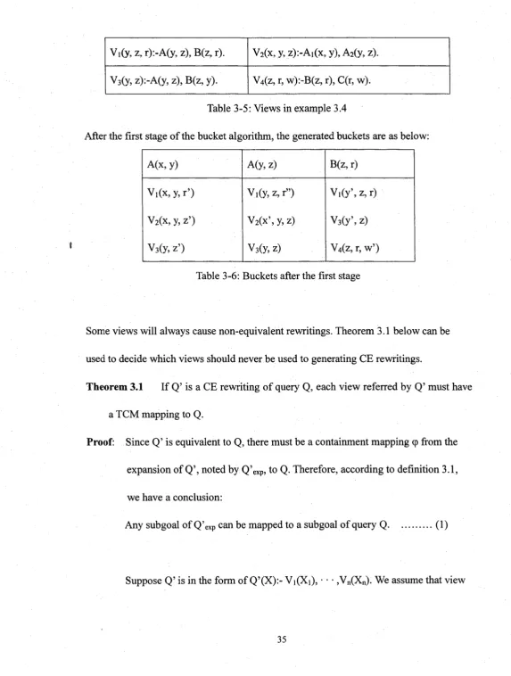
Example 3.4 Given a query Q(x, r):-A(x, y), A(y, z), B(z, r)., and four views as

(45)

Vi(y, z, r):-A(y, z), B(z, r). V2(x, y, z):-Ai(x, y), A2(y, z).

V3(y, z):-A(y, z), B(z, y). V4(z, r, w):-B(z, r), C(r, w).

Table 3-5: Views in example 3.4

After the first stage of the bucket algorithm, the generated buckets are as below:

A(x, y) A(y, z) B(z, r)

V i(x ,y ,r’)

V2(x, y, z ’)

V3(y ,z ’)

V i(y ,z ,r”)

V2(x’, y, z)

v 3( y , z)

Vi(y’, z, r)

V3(y’,z )

V4(z, r, w ’)

Table 3-6: Buckets after the first stage

Some views will always cause non-equivalent rewritings. Theorem 3.1 below can be

used to decide which views should never be used to generating CE rewritings.

Theorem 3.1 If Q’ is a CE rewriting o f query Q, each view referred by Q’ must have

a TCM mapping to Q.

Proof: Since Q ’ is equivalent to Q, there must be a containment mapping cp from the

expansion of Q \ noted by Q ’exp, to Q. Therefore, according to definition 3.1,

we have a conclusion:

Any subgoal of Q ’exp can be mapped to a subgoal of query Q... (1)

(46)

Vi( X;):- Si( Yi), • • • ,Sm( Ym) does not have TCM mapping to Q. So there

must be a subgoal of view Vj, say S( Y) that can not be mapped any subgoal of

Q-Suppose in the Q ’exp, subgoal S(yi,...,yn) of Vj is changed to S(zi,...,zn), where

Zj is renamed from yb 1 < i < n. There are two cases of zb

a) Variable Zj is a fresh new variable in Q ’exp, which means Zj does not

appear in any views other than Vj. Then R(zi, Q ’exp ) = R(yi,vo.

b) Variable z; is a variable in Q, so that R(zb Q ’exp)= R(yi,Vj) U ... U R(xn,

Vn), where xn is the variable in view Vn that is also renamed to zb Then

we have R(zi, Q’exp) e R (y i5Vi).

Based on a) and b), for any variable yi of subgoal S(yi,...,yn), R(zb Q ’eXp) £

R(yi,Vi), where Zj is the corresponding variable in subgoal S(zi,...,Z n). Thus we

can draw another conclusion:

A subgoal S(yi,.. .,yn) in view Vj can be mapped to the corresponding subgoal

S (Z i,...,Z n ) in Q exp- ...( 2 )

While according to conclusion (1), subgoal S(zi,...,zn) can be mapped to a

subgoal, say it is Sq, of Q. Then it is easy to infer that S(yi,.. .,yn) can also be

(47)

mapped to any subgoal of Q. It means that any view Vi must have a TCM

mapping to Q.

Q.E.D.

Intuitively speaking, Theorem 3.1 proves that views having no TCM mapping to a query

Q can never be used to generate CE rewritings of Q, no matter how they are combined

with other views. Based on the theorem 3.1, we develop the first rule of our algorithm,

i Rule 1: If a view does not have a TCM mapping to the given query, remove it before

running the bucket algorithm.

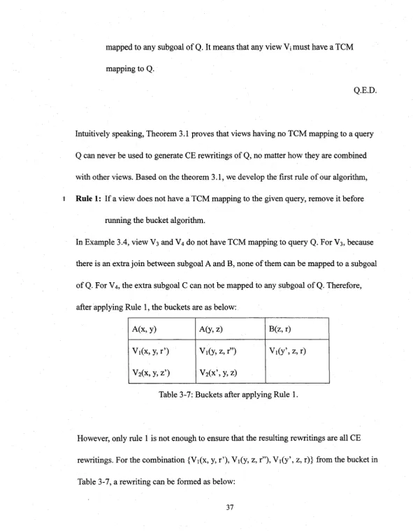
In Example 3.4, view V 3 and V 4 do not have TCM mapping to query Q. For V 3 , because

there is an extra join between subgoal A and B, none of them can be mapped to a subgoal

of Q. For V 4 , the extra subgoal C can not be mapped to any subgoal of Q. Therefore,

after applying Rule 1, the buckets are as below:

A(x, y) A(y, z) B(z, r)

V i(x ,y ,r’)

V2(x, y, z ’)

V i(y, z, r”)

V2( x \ y, z)

Vi(y’,z ,r )

Table 3-7: Buckets after applying Rule 1.

However, only rule 1 is not enough to ensure that the resulting rewritings are all CE

rewritings. For the combination {Vi(x, y, r ’), Vi(y, z, r”), V i(y’, z, r)} from the bucket in

(48)

Q i’(x, r):- Vi(x, y, r ’), Vi(y, z, r ” ), V i(y \ z, r).

After optimization, Q i’ becomes:

Q’i(x, r)> Vi(x, y, r ’), Vi(y, z, r).

Q’i.eXp(x, r):-A(x, y), B(y, r ’), A(y, z), B(z, r).

Q’i is a properly contained rewriting, i.e. Q’icQ , because in the expansion of Q’i,

subgoal B(y, r ’) cannot be mapped to any subgoal of Q.

In order to prevent generating a contained rewriting like Q ’ i, we need to refine the TCM

mapping to Bucket-TCM mapping as below.

Definition 3.4 (Bucket-TCM mapping)

Given a bucket (or subgoal) S(xj, x f in query Q, and a subgoal S(yi,...,yn) in a

view V. A mapping cp is a Bucket-TCM mapping from V to Q wrt S ( x i ,x j if

• S(yi, ...,yr) is mapped to the subgoal S(xj, x„); and

• All other subgoals in V are mapped to some subgoals in Q.

Different from the TCM mapping, Bucket-TCM mapping is relevant to one particular

subgoal. Through this definition, we are aware of that Vi does not have a Bucket-TCM

mapping to Q wrt the bucket S(x, y), hence Vi cannot be added to this bucket.

Generalizing from this observation, we developed the following theorem:

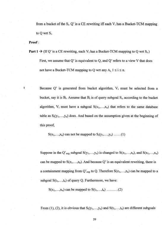
Theorem 3.2 Given a rewriting Q ’:-Vi, • • •, Vn. of query Q:-Si, ..., Sn., the rewriting

(49)

from a bucket of the Si. Q’ is a CE rewriting iff each Vj has a Bucket-TCM mapping

to Q wrt Sj.

Proof:

Part 1 (If Q ’ is a CE rewriting, each Vj has a Bucket-TCM mapping to Q wrt Sj.)

First, we assume that Q ’ is equivalent to Q, and Q ’ refers to a view V that does

not have a Bucket-TCM mapping to Q wrt any Ai; 1 < i < n.

* Because Q’ is generated from bucket algorithm, Vj must be selected from a

bucket, say it is Bj. Assume that Bj is of query subgoal Sj, according to the bucket

algorithm, V; must have a subgoal S(xi,...,xn) that refers to the same database

table as Sj(yi,...,yn) does. And based on the assumption given at the beginning of

this proof,

S(xi,...,xn) can not be mapped to Sj(yi,...,yn) ...(1)

Suppose in the Q ’eXp, subgoal S (yi,.. .,y„) is changed to S (zi,.. ,,zn), and S(xi,.. .,xn)

can be mapped to S(zi,... ,zn). And because Q’ is an equivalent rewriting, there is

a containment mapping from Q’eXp to Q. Therefore S (zi,.. ,,zn) can be mapped to a

subgoal S (ti,...,tn) of query Q. Furthermore, we have:

S(xi,... ,xn) can be mapped to S(ti,... ,tn) ... (2)

(50)

of query Q.

On the other hand, because Q ’ is an equivalent rewriting of query, the bucket

algorithm ensures that there is a containment mapping for Q to Q ’eXp that maps

subgoal S(yi,...,yn) to S(zi,...,zn), which means S i(yi,...,yn) can be mapped to

S(zi,...,zn). Because S(zi,...,zn) can be mapped to query subgoal S(ti,...,tn), the

conclusion can be drawn that Si(yi,...,yn) can be mapped to S(ti,...,tn). As

Si(yi,...,yn) and S (ti,...,tn) are different subgoals of Q , it can be proved that

Si(yi,...,yn) is redundant in query Q . This is contradictory to the earlier

assumption in this paper that no queries contain redundant subgoals.

In conclusion, the assumption at the beginning of this proof is not true.

Part 2 4r (If each V j has a Bucket-TCM mapping to Q wrt S j , Q ’ is a C E rewriting.)

Because the bucket algorithm guarantees that Q ’ is a complete rewriting and Q ’ c ; Q ,

we only need to prove Q c Q ’.

Because there is TCM mapping from Vj to Q , upon Theorem 3.1, any subgoal

S(xi,...,xm) ofV j can be mapped to a subgoal S(yi,. ..,ym) of Q , which means for any

(51)

Suppose in the Q’exp, subgoal S(xi,..,,xm) is changed to S (zi,...,zm), and variable zj,

1< j < m, is renamed from Xj using following rule:

a) If Xj is not a distinguished variable from subgoal S v i , Zj is a fresh variable in Q ’ eXp which does not appear in subgoals from views other than V j . So R ( z j ,

Q ’exp) = R ( X J , V i ) c R ( y j , Q ) .

b) If Xj is a distinguished variable from subgoal Svi, Xj is renamed to y ], i.e. Zj =

yj. According to the bucket algorithm, all variables that are mapped to yj are

renamed to Zj. So R(Zj, Q ’eXp) = R(xj, V j ) U ... U R(t, V t) . Because Svi can be

mapped to S q i, R(xj, V j ) c=R(yj, Q), same as all other variables that are

renamed to zj. So R(zj, Q ’exp) cR (yj5 Q).

Based on the two situations a) and b) above, any subgoal of V i in Q ’eXp can be

mapped to a subgoal of query Q . Similarly, all other subgoals in Q ’exp can also be

mapped to subgoals in query Q . Based on Definition 3.1, there is a TCM mapping

from Q ’exp to Q .

In addition, the bucket algorithm guarantees that all the head variables of Q ’exp have

1:1 map to the head variables of query Q. Overall, a conclusion can be drawn that

there is a containment mapping from Q ’eXp to Q, which proves Q c Q ’.

(52)

Based on Theorem 3.2, we develop the second rule for our algorithm:

Rule 2: When a view V is added to a bucket A of query Q, V must have a Bucket-TCM

mapping to Q wrt A.

For the buckets in Table 3-7, the only view that does not satisfy rule 2 is view Vi(x, y, r ’)

in the bucket of A (x, y). It can be verified that subgoal A(y, z) of Vi can only be mapped

to subgoal A(y, z) of Q, but not A(x, y) of Q. Based on rule 2, Vi should not be added to

the bucket of A(x, y). After rule 2 is applied, the buckets in Table 3-7 are changed as

below:

Ai(x, y) A2(y,z) B(z, r)

V2(x, y, z ’) V i(y, z, r”)

V2(x’, y, z)

Vi(y’,z ,r )

Table 3-8: Buckets after applying rule 2

In the combination stage of the bucket algorithm, with the buckets in Table 3-8, two

rewritings are generated as below. It can be verified that both Q’ 2 and Q’ 3 are CE

rewritings.

Q’2(x, r):-V2(x, y, z ’), Vi(y, z, r).

Q ’2-exP( x , r):-Ai(x, y), A2(y, z’), A(y, z), B(z, r).

Q’3(x, r):-V2(x, y, z), V i(y’, z, r).

(53)

Theorem 3.1 and 3.2 prove that by applying rule 1 and 2 in the first stage of the standard

bucket algorithm, the algorithm only produces CE rewriting. We refer to this expanded

bucket algorithm as TCM Bucket algorithm. Many rewritings that can be generated using

standard bucket algorithm will not be produced by TCM bucket algorithm.

According to Theorem 3.2, none of those rewritings are equivalent to the original query.

In another word, all CE rewritings that the standard bucket algorithm can create are also

1 in the output o f our TCM Bucket algorithm. Because the bucket algorithm can always

produce maximally contained rewriting, if there exist CE rewritings, the bucket

algorithm is guaranteed to find one. The same conclusion applies to TCM bucket

algorithm.

3.4.3 TCM Bucket Algorithm Implementation

The TCM bucket algorithm expands the bucket algorithm, so that all produced rewritings

are automatically CE rewritings without extra containment checking. Based on the first

stage of bucket algorithm, TCM bucket algorithm needs to apply an extra TCM mapping

to test which view should be put into which bucket.

First, we need to implement a procedure to find TCM mapping from a view to the given

(54)

that there is a TCM mapping from V to Q falls into two steps.

In the first step, the algorithm attempts to find out all possible mappings from variables

of V to variables of Q that cover all subgoals of view V. It first creates a matching set for

each subgoal of V. Every matching set contains all subgoals of Q that refer to the same

database relation as the corresponding view subgoal does. If any matching set is empty,

which means the view has an extra subgoal that does not exist in query Q, the

verification fails immediately, because in that case, there would be no tail containment

mapping from Q to V.

Here we use the query Q and view Y i in Example 3 to illustrate the procedure of finding

TCM mappings.

Q(x, r):-A(x, y), A(y, z), B(z, r).

Vi(y, z, r):-A(y, z), B(z, r).

The matching set o f the two subgoals A(y, z) and B(z, r) are as in Table 3-9,

A(y,z) A(x, y), A(y, z)

B(z, r) B(z, r)

Table 3-9: Matching sets for subgoals of view VI

Then, the procedure selects one subgoal from each matching set, and constructs a

mapping from the view subgoals to those query subgoals. As for the example above, two

(55)

V, A(y, z) B(z, r) y z r

<Pi(Vi) A (x,y) B(z, r) X _y r

CP2(Vl) A(y, z) B(z, r) _y z r

Table 3-10: Constructed mappings

In the second step, we check all mappings found in the first step, to see if there exists a

tail containment mapping. For view Vi, (pi is not a tail containment mapping, because cpi

maps subgoal B(z, r) to B(y, r) which is not included in query Q. Mapping 9 2

satisfies all conditions required to be a tail containment mapping.

To apply rule 1, TCM mapping verification procedure is used to test each view. If a view

V does not have any TCM mapping to Q, V will not be added to any bucket.

To apply rule 2, we make use of the TCM mappings found in the previous step. If there is

a Bucket-TCM mapping from V to Q wrt the query subgoal o f the bucket, the head o f V will be

(56)

The whole TCM bucket algorithm is described as in Figure 3-1.

/* TCM bucket algorithm*/

Begin

/* The first stage*/

For every view V in the bucket set B

Call TCM mapping verification procedure

If there is NO TCM mapping from V to Q

Continue Else

For every bucket Bi of query subgoal Si

If has a Bucket-TCM mapping to Qwrt Si

Rename head variables o f V Add V into Bi

Endif Endfor Endif Endfor

/* The second stage*/

Execute the combination stage algorithm of the bucket algorithm with bucket sets B to generate CE rewritings.

End

Figure 3-1: TCM bucket algorithm

In fact, the two rules in TCM bucket algorithm can also be applied to other bucket based

algorithms, such as MiniCon, SVB Bucket, etc. Since all bucket based algorithms consist

o f bucket construction stage and combination stage, it is very easy to apply the two rules

Complete and equivalent query rewriting using views.

Scholarship at UWindsor

Scholarship at UWindsor

Complete and equivalent query rewriting using views.

Complete and equivalent query rewriting using views.

C

o m p l e t e

a n d

E

q u i v a l e n t

Q

u e r y

R

e w r i t i n g

u s i n g

v i e w s

Abstract

Acknowledgements

Table of Contents

-List of Tables

List of Figures

Chapter 1

Introduction

1.1 Application Background

1.2 Data Integration

1.2.1 Introduction

1.2.2 Data Source Modeling

1.3 Query Rewriting Using Views

1.4 Thesis motivation and contribution

1.5 Thesis overview

Chapter 2

Overview of Query Rewriting Using Views

2.1

Query Language

P r o f

(pname, area)

A dvise(pna

me .snum)

'Course

(cnum, ctitle)

S tu dent

(simiiijSiianiejiiajo

Teachfpnau

f)

R eg iste r

(si

ie, cnum, term)

turn.cnum. term)'

pname

snum

Advise

S tu d e n t^ sname

major

Register

Course

/

V

cnum

ctitle

2.2 Query Rewriting

2.2.1 Query Containment and Equivalence

2.2.2 Containment Mapping

2.2.3 Query Rewriting Using Views

• G’« 0 .

2.2.4 Query Expansion

2.2.5 Rewriting Containment Verification

2.3 Previous Algorithms for Query Rewriting

Chapter 3

Finding Complete and Equivalent Rewriting

3.1 Motivation

3.2 Expanding equivalent rewriting algorithms

3.3 Expanding Complete Rewriting Algorithms

3.4 TCM Bucket Algorithm

3.4.1 Definitions

3.4.2 Expanding Bucket Algorithm with TCM

3.4.3 TCM Bucket Algorithm Implementation