| INVESTIGATION
Bayesian Estimation of Population Size Changes by
Sampling Tajima
’
s Trees
Julia A. Palacios,*,†,1Amandine Véber,‡Lorenzo Cappello,* Zhangyuan Wang,§John Wakeley,** and Sohini Ramachandran††,‡‡ *Department of Statistics and§Department of Computer Science, Stanford University, and†Department of Biomedical Data Science, Stanford School of Medicine, California 94305,‡Centre de Mathématiques Appliquées, École Polytechnique 91128, Le Centre National de la Recherche Scientifique, Palaiseau, France 91767, **Department of Organismic and Evolutionary Biology, Harvard University, Cambridge, Massachusetts 02138, and††Center for Computational Molecular Biology and‡‡Department of Ecology and Evolutionary Biology, Brown University, Providence, Rhode Island 02912
ABSTRACTThe large state space of gene genealogies is a major hurdle for inference methods based on Kingman’s coalescent. Here, we present a new Bayesian approach for inferring past population sizes, which relies on a lower-resolution coalescent process that we refer to as “Tajima’s coalescent.” Tajima’s coalescent has a drastically smaller state space, and hence it is a computationally more efficient model, than the standard Kingman coalescent. We provide a new algorithm for efficient and exact likelihood calculations for data without recombination, which exploits a directed acyclic graph and a correspondingly tailored Markov Chain Monte Carlo method. We compare the performance of our Bayesian Estimation of population size changes by Sampling Tajima’s Trees (BESTT) with a popular implementation of coalescent-based inference in BEAST using simulated and human data. We empirically demonstrate that BESTT can accurately infer effective population sizes, and it further provides an efficient alternative to the Kingman’s coalescent. The algorithms described here are implemented in the R package phylodyn, which is available for download athttps://github.com/ JuliaPalacios/phylodyn.
KEYWORDSBayesian nonparametrics; coalescent; effective population size; Tajima coalescent
M
ODELING gene genealogies from an alignment of se-quences (timed and rooted bifurcating trees reflecting the ancestral relationships among sampled sequences), is a key step in coalescent-based inference of evolutionary parame-ters such as effective population sizes. In the neutral coales-cent model without recombination, observed sequence variation is produced by a stochastic process of mutation acting along the branches of the gene genealogy (Watterson 1975; Kingman 1982a), which is modeled as a realization of the coalescent point process at a neutral non-recombining locus. In the coalescent point process, the rate of coalescence (the merging of two lineages into a common ancestor at some time in the past) is a function that varies with time, and it is inversely proportional to the effectivepopulation size at time t, NðtÞ (Kingman 1982b; Slatkin and Hudson 1991; Donnelly and Tavaré 1995). Our goal is to infer ðNðtÞÞt$0, which we will refer to as the“effective population size trajectory.”
Multiple methods have been developed to inferðNðtÞÞt$0 using the standard coalescent model with or without recom-bination. Some of these methods inferðNðtÞÞt$0 from sum-mary statistics such as the sample frequency spectrum (SFS) (Bhaskaret al.2015; Terhorstet al.2017); however, the SFS is not a sufficient statistic for inferringðNðtÞÞt$0 (Sainudiin
et al.2011). Other methods have been proposed that directly
use molecular sequence alignments at a completely linked locus, i.e., without recombination (Griffiths and Tavaré 1996; Kuhner and Smith 2007; Minin et al. 2008; Li and Durbin 2011; Drummond et al. 2012; Gill et al. 2013; Palacios and Minin 2013). Our approach is of this type. Still other methods account for recombination across larger geno-mic segments (Li and Durbin 2011; Sheehan et al. 2013; Schiffels and Durbin 2014; Palacioset al.2015). In spite of their variety, all these methods must contend with two major challenges: (1) choosing a prior distribution or functional Copyright © 2019 by the Genetics Society of America
doi:https://doi.org/10.1534/genetics.119.302373
Manuscript received May 28, 2019; accepted for publication September 6, 2019; published Early Online September 11, 2019.
Available freely online through the author-supported open access option.
form forðNðtÞÞt$0, and (2) integrating over the large hidden state space of genealogies. For example, several previous ap-proaches have assumed exponential growth (Griffiths and Tavaré 1996; Kuhneret al. 1998; Kuhner and Smith 2007), in which case the estimation ofðNðtÞÞt$0 is reduced to the estimation of one or two parameters. In general, the functional form of ðNðtÞÞt$0 is unknown and needs to be inferred. A commonly used naive nonparametric prior on ðNðtÞÞt$0 is a piecewise linear or constant function defined on time intervals of constant or varying sizes (Heled and Drummond 2008; Sheehanet al.2013; Schiffels and Durbin 2014). The specifi -cation of change points in such time-discretized effective pop-ulation size trajectories is inherently difficult because it can lead to runaway behavior or large uncertainty in ðN^ðtÞÞt$0. These difficulties can be avoided by the use of Gaussian process priors in a Bayesian nonparametric framework, allowing accu-rate and precise estimation (Gillet al.2013; Palacios and Minin 2013; Lanet al.2015; Palacioset al.2015). More precisely, the autocorrelation modeled with the Gaussian process avoids run-away behavior and large uncertainty inðN^ðtÞÞt$0.
The second challenge for coalescent-based inference of ðNðtÞÞt$0 is the integration over the hidden state space of genealogies for large sample sizes. Given molecular sequence dataYat a single nonrecombining locus and a mutation model with parameter m, current methods rely on calculating the marginal likelihood function PrðYðNðtÞÞt$0;mÞby integrat-ing over all possible coalescence and mutation events. Under the infinite sites mutation model without intralocus recombi-nation (Watterson 1975), this integration requires a computa-tionally expensive importance sampling technique or Markov Chain Monte Carlo (MCMC) techniques (Griffiths and Tavaré 1994a; Stephens and Donnelly 2000; Hobolthet al.2008; Wu 2010; Gronauet al.2011). Moreover, a maximum likelihood estimate ofðNðtÞÞt$0cannot be explicitly obtained; instead, it is obtained by exploring a grid of parameter values (Tavaré 2004). Forfinite sites mutation models, current methods ap-proximate the marginal likelihood function by integrating over all possible genealogies via MCMC methods [Equation 1; Kuhner (2006); Drummondet al.(2012)]. In both cases, the marginal likelihood may be expressed as
PrYjðNðtÞÞt$0;m
¼
Z
PrðYjg;mÞPrgjðNðtÞÞt$0
dg; (1)
in which PrðÞis used to denote both the probability of dis-crete variables and the density of continuous variables. The integral above involves anðn21Þ-dimensional integral over n21 coalescent times and a sum over all possible tree topol-ogies withnleaves. Therefore, these methods require a very large number of MCMC samples, and exploration of the pos-terior space of genealogies continues to be an active area of research (Kuhner et al. 1998; Rannala and Yang 2003; Drummondet al.2012; Whidden and Matsen 2015; Aberer et al.2016).
Current methods rely on the Kingmann-coalescent process to model the sample’s ancestry. However, the state space of
genealogical trees grows superexponentially with the num-ber of samples, making inference computationally challeng-ing for large sample sizes. In this study, we develop a Bayesian nonparametric model that relies on Tajima’s coales-cent, a lower-resolution coalescent process with a drastically smaller state space than that of Kingman’s coalescent. In particular, we approximate the posterior distribution PrððNðtÞÞt$0;gT;tjY;mÞ, wheregT corresponds to the Taji-ma’s genealogy of the sample (see Figure 1A andTajima’s genealogies),ðlog NðtÞÞt$0has a Gaussian process prior with precision hyperparametertthat influences the smoothness of the resulting trajectory, and mutations occur according to the infinite sites model of Watterson (1975). This results in a new efficient method for inferring ðNðtÞÞt$0 called
Bayesian Estimation bySamplingTajima’sTrees (BESTT), with a drastic reduction in the state space of genealogies. Using simulated data, we show that BESTT can accurately infer effective population size trajectories and that it pro-vides a more efficient alternative than Kingman’s coalescent models.
Next, we start with an overview of BESTT, detail our representation of molecular sequence data, and define the Tajima coalescent process. We then introduce a new aug-mented representation of sequence data as a directed acyclic graph (DAG). This representation allows us to both calculate the conditional likelihood under the Tajima coalescent model and to sample tree topologies compatible with the observed data. We then provide an algorithm for likeli-hood calculations and develop an MCMC approach to effi -ciently explore the state space of unknown parameters. Finally, we compare our method to other methods imple-mented in Bayesian Evolutionary Analysis Sampling Trees (BEAST) (Drummond et al.2012) and estimate the effec-tive population size trajectory from human mitochondrial DNA (mtDNA) data. We close with a discussion of possible extensions, and limitations of the proposed model and implementation.
Materials and Methods
Overview of BESTT
likelihood, Equation 1, will differ only by a combinatorial factor from the corresponding likelihood under the Kingman coalescent. Our DAG represents the data with a gene tree (Griffiths and Tavaré 1994a), constructed via a modified ver-sion of the perfect phylogeny algorithm of Gusfield (1991). This provides an economical representation of the uncer-tainty, and conditional independences induced by the model and the observed data.
Under the infinite sites mutation model, there is a one-to-one correspondence between observed sequence data and the gene tree of the data (Gusfield 1991) (Summarizing
sequence data Y as haplotypes and mutation groups and
Representing Yh3m as a gene tree). We further augment
the gene tree representation with the allocation of the num-ber of observed mutations along the Tajima’s genealogy to generate a DAG (An augmented data representation using directed acyclic graphs). The conditional likelihood PrðYjgT;mÞ is then calculated via a recursive algorithm that exploits the auxiliary variables defined in the DAG nodes, marginalizing over all possible mutation allocations (Computing the conditional likelihood). We approximate the joint posterior distribution PrððNðtÞÞt$0;gT;tjY;mÞvia an MCMC algorithm using Hamiltonian Monte Carlo for sam-pling the continuous parameters of the model and a novel Metropolis–Hastings algorithm for sampling the discrete tree space.
Summarizing sequence dataYas haplotypes and
mutation groups
Let the data consist of nfully linked haploid sequences or alignments of nucleotides atssegregating sites sampled from nindividuals at timet¼0 (the present). Note that any labels we affix to the individuals are arbitrary in the sense that they will not enter into the calculation of the likelihood. We fur-ther assume the infinite sites mutation model of Watterson (1975) with mutation parameter m and known ancestral states for each of the sites. Then, we can encode the data into a binary matrix Y ofn rows ands columns with elements yi;j2 f0;1g, where 0 indicates the ancestral allele.
To calculate the Tajima’s conditional likelihood PrðYjgT;mÞ, wefirst record each haplotype’s frequency and group repeated columns to formmutation groups; a mutation group corresponds to a shared set of mutations in a subset of the sampled individuals. We record the cardinality of each mutation group (i.e., the number of columns that show each mutation group). In Figure 2A, there are two columns labeled “b,” corresponding to two segregating sites that have the exact same pattern of allelic states across the sample. Fur-ther, two individuals carry the derived allele of mutation group b, so in this case the frequency of haplotype 7 and the cardinality of mutation group b are both equal to 2. Like-wise, haplotype 4 has frequency 1 and carriesfive mutations that are split into mutation groups“a,” “f,”and“g”(the latter is not shown in Figure 2A, but appears in Figure 2B) of re-spective cardinalities 1, 3, and 1. We denote the number of haplotypes in the sample as h, the number of mutation groups asm, and the representation ofYas haplotypes and mutation groups asYh3m.
RepresentingYh3m as a gene tree
Yh3m(Figure 2A) can alternatively be represented as a gene tree or perfect phylogeny (Gusfield 1991; Griffiths and Tavaré 1994b). This representation relies on our assumption of the infinite sites mutation model in which, if a site mutates once in a given lineage, all descendants of that lineage also have the mutationand no other individuals carry that muta-tion. The gene tree is a graphical representation of the hap-lotypes (as tips) arranged by their patterns of shared mutations. The haplotype data summarized in Figure 2A cor-respond to the gene tree given in Figure 2B. Details of the correspondence between haplotype data and gene tree are listed below, and an additional example is given in Figure E1 (Appendix E).
Agene treefor a matrixYh3m ofhhaplotypes andm
mu-tation groups is a rooted treeT withhleaves and at leastm edges, such that (Figure 2B):
1. Each row ofYh3m corresponds to exactly one leaf ofT. The black numbers at leaf nodes in Figure 2B are the haplotype frequencies.
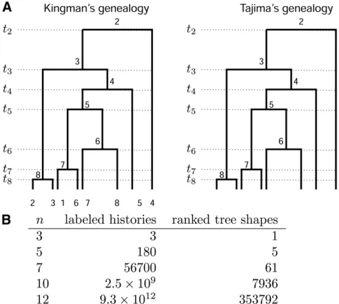
2. Each mutation group of Yh3m is represented by exactly one edge of T, which is labeled accordingly (letters in Figure 2, A and B). The red numbers along edges in Figure Figure 1 For a sample of sizen, the number of Tajima’s genealogies is
superexponentially fewer compared to the number of Kingman’s gene-alogies. (A) A Kingman’s genealogy and a Tajima’s genealogy forn¼8. A Kingman’s genealogy (left) comprises a vector of coalescent times and the labeled topology; the number of possible labeled topologies for a sample of sizenisn!ðn21Þ!=2n21. A Tajima’s genealogy (right)
com-prises a vector of coalescent times and a ranked tree shape. In both cases, coalescent events are ranked from 2 at timet2tonat timetn. Coalescent
2B give the cardinality of each mutation group (i.e., the number of segregating sites in this group; see Figure 2A). Some external edges (edges subtending leaves) may not be labeled, indicating that they do not carry additional mutations to their parent edge. This happens when the other edges emanating from the parent node necessarily correspond to other mutation groups.
3. Edges are placed in the gene tree in such a way that each “path”from the root to a leaf fully describes a haplotype.
Edges corresponding to shared mutations between several haplotypes are closest to the root. For example, in Figure 2B, haplotype 4 corresponds to the leaf at which one ar-rives starting from the root and going along edges a, g, and f; in contrast, haplotype 7 corresponds to the leaf at which one arrives going from the root along edge b. Thus, the labels and the numbers associated with the edges along the unique path from the root to a leaf exactly specify a row ofYh3m.
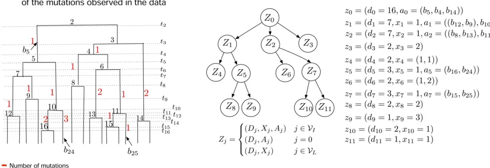
Figure 2 Data structures employed by our method, Bayesian Estimation of population size changes by Sampling Tajima’s Trees (BESTT), for calculating the conditional likelihood of the data. (A) Compressed data representationYh3mofn¼16 sequences ands¼18 (columns, only thefirst 10 of which
are shown), comprised of nine haplotypes and 13 mutation groups. Rows correspond to haplotypes and each polymorphic site is labeled by its mutation groupfa;b;c;. . .;mg. (B) Gene tree representation of the data in (A). Red numbers indicate the cardinality of each mutation group [number of columns with the same label in (A)]. Black letters indicate the mutation group [column labels in (A)], and black numbers indicate the frequency of the corresponding haplotype. (C) A Tajima’s genealogy compatible with the gene tree in (B). Internal nodes are labeled according to order of coalescent events from the root to the tips. Coalescent eventihappens at timetiand branches are labeledbi(seeAn augmented data representation using
directed acyclic graphsfor details). (D) A Directed Acyclic Graph (DAG) representation of the gene tree in (B) together with allocation of mutation groups along the branches of the Tajima’s genealogy in (C).VIdenotes the set of internal nodes andVLthe set of leaf nodes. A detailed description of the DAG
Dan Gusfield’s perfect phylogeny algorithm (Gusfield 1991) transforms the sequence dataYh3minto a gene tree and this transformation is one-to-one. We note that the perfect phylogeny T or gene tree is not the same as the genealogy g. While a genealogy is a bifurcating tree of individuals of the sample, the gene tree is a multifurcating tree of haplotypes.
Tajima’s genealogies
Our method of computing the probability of the recoded data,
Yh3m, uses ranked tree shapes rather than fully labeled
histo-ries. We refer to these ranked tree shapes as Tajima’s geneal-ogies but note they have also been calledunlabeled rooted trees (Griffiths and Tavaré 1995) and evolutionary relationships (Tajima 1983). In Tajima’s genealogies, only the internal nodes are labeled and they are labeled by their order in time. Tajima’s genealogies encode the minimum information needed to compute the probability of data Yh3m, which consists of
nested sets of mutations, without any approximations. In Fig-ure 1A for example, it matters only that mutation group e occurs on a subgroup of the individuals who carry mutation group“a,”and that this is different from the subgroups carrying c, d, and f. No other labels matter because individuals are exchangeable in the population model we assume.
This represents a dramatic coarsening of tree space com-pared to the classical leaf-labeled binary trees of Kingman’s coalescent. The number of possible ranked tree shapes for a sample of sizencorresponds to then-th term of the sequence A000111 of Euler zig-zag numbers (Disanto and Wiehe 2013) whereas the number of labeled binary tree topologies is n!ðn21Þ!=2n21. As can be seen from Figure 1B, this pro-vides a much more efficient way to integrate over the key hidden variable, the unknown gene genealogy of the sample, when computing likelihoods.
We model this hidden variable using thevintaged and sized
coalescent(Sainudiinet al.2015), which corresponds exactly
to this coarsening of Kingman’s coalescent. As can be seen in Figure 1A, we assign vintages/labels 2 throughnstarting at the root of the tree and moving toward the present, so that the node created by thefinal splitting event, which is also the
first coalescence event looking back in the ancestry of the sample, is labeled n. We write tk for the time of node k, measured from the present back into the past. We set tnþ1:¼0 to be the present time. Then during the interval ½tkþ1;tkÞ the sample has exactly k extant ancestors, for k2 f2;. . .;ng.
The coarsening of the tree topology does not change the law of the times between two coalescence events. Thus, conditional on the effective population size trajectory ðNðtÞÞt$0and the timetkþ1at which the number of ancestors to the sample decreases to k, the distribution of the time during which the sample haskancestors is given by
Prtk2tkþ1jtkþ1;ðNðtÞÞt$0
¼ Ck
NðtkÞ
exp
2
Z
tk tkþ1
Ck
NðtÞdt
(2)
(Slatkin and Hudson 1991), where Ck¼
k 2
. Writing the density att¼ðt2;t3;. . .;tnÞof the vector of coalescence times as a product of conditional densities, we obtain
PrtjðNðtÞÞt$0
¼Y n
k¼2
Prtk2tkþ1jtkþ1;ðNðtÞÞt$0
: (3)
We use a lower triangular matrix denoted F to represent Tajima’s genealogies; see Appendix A. The probability of a ranked tree shape was derived independently in Sainudiin et al.(2015) and Palacioset al.(2015). Specifically, for every ranked tree shapeFwithnleaves,
PrðFÞ ¼ 2 n2c21
ðn21Þ!; (4)
wherecis the number of cherries inF(i.e., nodes subtending two leaves;c¼3 in Figure A1A). Note that this probability is independent of the effective population size trajectory since the choice of the pair of lineages that coalesce during an event is independent of ðNðtÞÞt$0 (recall that in King-man’s coalescent, the coalescing pair is chosen uniformly at random among all possible pairs). Since the distribution of Tajima’s genealogies gT¼ ðF;tÞ conditional on ðNðtÞÞ
t$0 can be factored as the product of the probability of the ranked tree shape Fand the coalescent times density, we arrive at
PrgTjðNðtÞÞt$0
¼ 2n2c21 ðn21Þ!
Yn
k¼2
Ck
NðtkÞ
exp
2
Z
tk tkþ1
Ck
NðtÞ dt
: (5)
An augmented data representation using directed acyclic graphs
A key component of BESTT is the calculation of the conditional likelihood PrðYjgT;mÞ. We compute the conditional likeli-hood recursively over a DAG,D. Our DAG exploits the gene tree representation T of the data (Figure 2B), incorporates the branch length information of the Tajima’s genealogy
gT(Figure 2C), and facilitates the recursive allocation of mu-tations to the branches ofgT. Here, we detail the construction of the DAG.
Constructing the DAGD:The graph structure of our DAG
D¼ fZ;Eg(Figure 2D) with nodes Zand edges Eis con-structed from a gene treeT. The number of internal nodes in the DAGDis the same as the number of internal nodes in T. However, sister leaf nodes inT with the same number of descendants are grouped together in D and leaf nodes descending from edges with no mutations are treated as singletons grouped together inD. For example, the leaves in Figure 2B subtending from edgesiandjare grouped into Z6 in Figure 2D, as they both have haplotype frequency 2. However, the leaves subtending from the e and f edges are not grouped (and correspond toZ8 andZ9in the DAG Fig-ure 2D) since they have respective haplotype frequencies 2 and 1. We label the root node ofDasZ0and increase the indexiof each nodeZifrom top to bottom, moving left to right. Fori,j, we assign a directed edgeEi;jif the node inT corresponding to Zi is connected to the node inT corre-sponding to Zj. The index set of internal nodes in D is denoted by VI and the index set of leaf nodes is denoted byVL.
Information carried by the nodes in D: Each node in D
represents a vector, Zj, which includes number of descen-dants, number of mutations, and latent allocation of muta-tions. Although the number of descendants and number of mutations are part of the observed data, the allocation of mutations can be seen as a random variable; for ease of ex-position, we use capital letters to denote all three types of information. We define the vectorZjas follows:
Zj¼ 8 < :
ðDj;Xj;AjÞ j2 VI;
ðDj;AjÞ j¼0 ðthe root nodeÞ; ðDj;XjÞ j2 VL;
whereDjdenotes the number of descendants of (i.e., of sam-pled sequences subtended by) nodeZj,Xjdenotes the number of mutations separatingZjfrom its parent node, andAjdenotes the allocation of mutations alonggT (described in detail be-low). The number of descendants Dj is thus the number of individuals/sequences descending from nodeZj(this informa-tion is part ofT). For internal nodes,Xjrecords the cardinality of a mutation group, represented as a red number along the edgeEi;jofT in Figure 2B, whereiis the index of the parent node ofZj. Leaf nodes inDmay correspond to more than one leaf node inT, namely any sister nodes with the same number of descendants. In this case,Xjis a vector with the cardinalities of the corresponding mutation groups (see for example node Z6in Figure 3B). To keep the DAG construction simple, we only allow groupings of leaf nodes and not of internal nodes with identical descendants carrying identical numbers of mutations. We note that, in principle, it would be possible to compress the number of internal nodes of the DAG by exploiting all the symmetries observed in the data.
Allocation of mutation groups alonggT:The latent
alloca-tion variablesfAjgdetermine a possible correspondence be-tween subtrees in gT and nodes in D; in particular, Aj indicates the branches ingTthat subtend the subtrees corre-sponding to nodesfZkgiffZkgare child nodes ofZj.
Allocations of mutations to branches are usually not unique and computation of the conditional likelihood PrðYjgT;mÞ requires summing over all possible allocations. In Figure 3A we show one such possible allocation of the mutation groups of the gene tree in Figure 2B along the Tajima’s genealogy in Figure 2C. For example, mutation group a in Figure 2B with cardinality 1 (number in red) is a mutation observed in seven individuals (sum of black numbers of leaves descending from Figure 3 Directed Acyclic Graph (DAG) construction. (A) A Tajima’s genealogy from Figure 2C with added allocation of mutations shown in red. (B) The corresponding augmented DAG with allocation of mutations. At the rootZ0, there are no mutations by convention. NodeZ0has 16 descendants across
three subtrees of 7;7 and two descendants, corresponding to nodesZ1;Z2; and Z3. These three subtrees subtend fromb5;b4, andb14, respectively, ingT
(A). NodeZ1corresponds to the tree subtending fromb5of size 7 withX1¼1 mutation alongb5, and subtends three subtrees fromðb12;b9Þandb10.
Subtrees subtending fromðb12;b9Þare grouped together in leaf nodeZ4because they both have two descendants and have the same parent node. When
edge marked a). This same mutation group, a, is shown as a red number 1 in Figure 3A allocated to branchb5. IfZjis an internal node, the number of mutations Xjis denoted as a vector of length 1. IfZjis a leaf node,Xjcan be a vector of length.1. Details on notation for allocations can be found in Appendix B.
Computing the conditional likelihood
Under the infinite sites mutation model, mutations are super-imposed independently on the branches ofgT as a Poisson process with ratem. To compute PrðYjgT;mÞ ¼PrðT jgT;mÞ, we marginalize over the latent allocation information in the DAGD; that is, we sum over all possible mappings of muta-tions inT to branches ingTas follows:
PrYjgT;m¼X A0
X
A1 . . .X
AnI
PrDjgT;m
¼X A0
X
A1 . . .X
AnI
PrZ0;. . .;ZnIþnLjg
T;m
¼X A0
X
A1 . . .X
AnI Y nIþnL
i¼1
Pr ZijZpaðiÞ;gT;m
wherenI¼ jVIj,nL¼ jVLj,paðiÞdenotes the index of the par-ent of nodeiinD, and we setPðZ0gT;mÞ ¼1 because it is assumed that there are no mutations above the root node and the length of the root branchl2¼0. WritingLfor the tree length ofgT(i.e., the sum of the lengths of all branches ofgT) and factoring out a global factor e2mL (due to the Poisson distribution of mutations across the genealogy) from each of the above products overi2 f1;. . .;nIþnLg, we have
where Pðxi;kÞ is the set of all permutations of xi¼ fxi1;. . .;xikgdivided into mi groups of different sizes. The number of different permutations of thekvalues ofxidivided intomigroups of sizesk1;. . .;kmiis
jPðxi;kÞj ¼
k!
Qmi
j¼1
kj!
: (6)
For example, assume that xi¼ f2;2;2;0;3;3g andapaðiÞ¼
ðb3;b4;b5;b6;b7;b8Þ with branch lengthsfl3;l4;l5;l6;l7;l8g. In this case,k1¼3 because there will be three branches with
two mutations,k2¼1 because there will be one branch with no mutations, andk3¼2 because there will be two branches with three mutations. The number of permutations ofk¼6 mutations groups divided intomi¼3 groups with cardinal-ities 2;0;3 of sizes 3;1;2 is 6!=ð3!1!2!Þ ¼60.
The conditional likelihood PrðYgT;mÞis calculated via a backtracking algorithm (Appendix C). The algorithm margin-alizes the allocations by traversing the DAG from the tips to the root. The pseudocode and an example can be found in Appendix C.
The case of unknown ancestral states
Up to now, we have assumed that the ancestral state was known at every segregating site. The representation of the data Ythat we use in this case records the cardinalities of each mutation group and the genealogical relations between these groups, but does not assign labels to the sequences. Hence, in the terminology of Griffiths and Tavaré (1995), our data corresponds to anunlabeled rooted gene tree.
When the ancestral types are not known, the data (now denoted Y0) may be represented as an unlabeled unrooted gene tree. By the remark following Equation 1 in Griffiths and Tavaré (1995), ifsis the number of segregating sites, then there are at mostsþ1 unlabeled rooted gene trees that cor-respond to the unrooted gene tree of the observed data ðRðY0ÞÞ. By the law of total probability [see also Equation 10 in Griffiths and Tavaré (1995)], the conditional likelihood ofY0can be written as the sum over all compatible unlabeled rooted gene treesYðiÞof the probability ofYðiÞconditionally
ongT. That is:
PrY0jgT;m¼ X
Rð ÞY0
i¼1
P Yð Þi jgT;m
; (7)
where each of the YðiÞ corresponds to a unique
unla-beled rooted gene tree compatible with the unrooted gene treeY0 andRðY0Þdenotes the number of those un-labeled rooted gene trees. In the following sections, we shall assume that the ancestral type at each site is known.
Pr Zi¼zijzpaðiÞ;gT;m
¼
(
Pr Xi¼xijapaðiÞ¼bj;gT;m
}ðmljÞxi if jxij ¼1;
PrðXi¼ ðxi1;. . .;xikÞÞ japaðiÞ¼ ðbj1;. . .;bjkÞ;g
T;m} X
s2Pðxi;kÞ Yk
m¼1
ðmljmÞ
sm if jx
Bayesian inference of the effective population size trajectory
Our posterior distribution of interest is
Prg;gT;tY;m}PrYgT;mPrgTgPrðgjtÞPrð Þt ; (8)
where logN tð ð ÞÞt$0¼ðgð ÞtÞt$0 GPð0;Cð Þt Þhas a Gauss-ian process prior with mean0and covariance functionCðtÞ
(Rasmussen and Williams 2006). This specification ensures ðNðtÞÞt.0is nonnegative. In our implementation, we assume a regular geometric random walk prior, that is, g1¼ logNðt*
1Þ;. . .;gB¼logNðtB*ÞatBregularly spaced time points in½0;Twith
Cov
h
gi;gji¼Cov
logN t*i
;logN t*j
¼t min t*i;t*j
:
The parametertis a length-scale parameter that controls the de-gree of smoothness of the random walk. We place agprior with parametersa¼0:01 andb¼0:001 ont, reflecting our lack of prior information in terms of high variance about the smoothness of the logarithm of the effective population size trajectory.
We approximate the posterior distribution of model pa-rameters via an MCMC sampling scheme. Model papa-rameters are sampled in blocks within a random scan Metropolis-within-Gibbs framework. Our algorithm initializes with the corresponding Tajima genealogy of the UPGMA estimated tree implemented in phangorn (Schliep 2011). Given an ini-tial genealogy, our algorithm iniini-tializes Ne and t with the method of Palacios and Minin (2012) implemented in phylo-dyn (Karcheret al.2017). We then proceed to generate: (1) a sample of the vector of effective population sizes and pre-cision parameter as described in Split Hamiltonian Monte Carlo updates ofðg;tÞ, (2) a sample of the vector of coales-cent times as described inHamiltonian Monte Carlo updates of
coalescent timesandLocal updates of coalescent timeswhere
we modify a single coalescent time, and (3) a sample of ranked tree shape as described in Metropolis–Hastings
up-dates for ranked tree shapesin each iteration. To summarize
the effective population size trajectory, we compute the pos-terior median and 95% credible intervals pointwise at each grid point in½0;T^, wereT^is the maximum time to the most recent common ancestor sampled.
Metropolis–Hastings updates for ranked tree shapes:There
is a large body of literature on local transition proposal distri-butions for Kingman’s topologies (Kuhneret al.1998; Rannala and Yang 2003; Drummondet al.2012; Whidden and Matsen 2015; Abereret al.2016). In this paper, we adapted the local transition proposal of Markovtsovaet al. (2000) to Tajima’s topologies. We briefly describe the scheme below and provide a pseudocode algorithm in Appendix C (Algorithm 3).
Given the current state of the chain g;t;gT¼
g;t;Fn;t
f g, we propose a new ranked tree shapeF*in two steps. For step 1, we first sample a coalescent intervalek¼ ðtkþ1;tkÞ uniformly at random, where kUðf3;. . .;ngÞ.
Note that we will never select the intervalðt3;t2Þat the top of the tree (see Figure A1A). Givenk, we focus solely on the coalescent events at timestkandtk21. For step 2, there are two possible scenarios. Case A: the lineage created at timetk, labeledk, coalesces at timetk21(first row of Figure 4A). Case B: lineage kdoes not coalesce at time tk21 (Figure 4B). In Case A, we choose a new pair of lineages at random to co-alesce at time tk from the three lineages subtending kand k21 (excludingk), and we coalesce the remaining lineage withkattk21(Fn*;1andFn*;2in Figure 4). In Case B, we invert the order of the coalescent events; that is, the two lineages descending fromkare set to coalesce at timetk21and line-ages descending fromk21 are set to coalesce at timetk(F*
n;3 a in Figure 4). Note that the numerical labels 1;2;3 are in-cluded to clarify the picture: lineages subtending both Case A and Case B can be either labeled (if there is a vintage sub-tending that lineage) or not (if there is a singleton). The transition probabilityqðF*
nFnÞis given by the product of the probabilities of the two steps. The new ranked tree shapeF*
nis accepted with probability given by the Metropolis–Hastings ratio defined below:
aFn¼min 1;
Pr YjF*
n;t;m
Pr F*
n q FnjF*n
PrðYjFn;t;mÞPrð ÞFn q F*njFn
( )
: (9)
We note that our proposal can result in the same ranked tree shape. However, we tested alternative proposals that pre-cluded this event and we did notfind any notable difference in the overall performance of the MCMC algorithm.
Split Hamiltonian Monte Carlo updates ofðg;tÞ:To make
efficient joint proposals ofgandt, we use the Split Hamilto-nian Monte Carlo method proposed by Lan et al. (2015). Figure 4 Markov moves for topologies. First row: possible coalescent pat-terns (Case A or Case B) for a given topology Fn. Second row: possible
Markov moves in Case A (F*
n;1andFn*;2) and Case BðFn*;3Þ.kindexes the
coalescent interval sampled. Numerical labels at the tips are added for con-venience: conditionally on a givenFn, tips can be labeled (vintage) or not
Conditioned ongT, the target density becomespðg;tÞ}PrðtjgÞ PrðgjtÞPrðtÞ. This is the same target density implemented in Karcheret al.(2017) forfixed coalescent timest.
Hamiltonian Monte Carlo updates of coalescent times:
Given the current statefg;t;gTg ¼ fg;F
n;t;tg, we propose a new vector of coalescent times with target density
pðt9Þ}PðYjFn;t9;mÞPðt9jgÞby numerically simulating a Ham-ilton system with HamHam-iltonian
Hðlogðt9Þ;sÞ ¼ 2logðpðlogðt9ÞÞÞ þ1
2s
TMs; (10)
where s is the momentum vector assumed to be normally distributed. The system evolves according to:
@s
@x¼=logpðlogðt9ÞÞÞ
@t0
@x¼Ms: (11)
We use theleapfrogmethod (Neal 2011) with step sizeeand a p Poisson with mean 10 distributed number of steps to simulate the dynamics from timex¼0 tox¼pe. Each leap-frog step of sizeefollows the trajectory:
sxþe 2 ¼sxþ
e
2=logpðlogðt 0
xÞÞÞ
t0xþe¼t0xþeMsxþe 2
sxþe¼sxþe 2 þ
e
2=logpðlogðt 0
xþeÞÞÞ: (12)
For our implementation, we set the mass matrixM¼I, the identity matrix. We simulate the Hamiltonian dynamics of the logarithm of times to avoid proposals with negative val-ues. Solving the equations of the Hamilton system requires calculating the gradient of the logarithm of the target density with respect to the vector of log coalescent times. The gradi-ent of the log conditional likelihood (score function) is cal-culated at every marginalization step in the algorithm for the likelihood calculation.
At the beginning ofBayesian inference of the effective
pop-ulation size trajectory, we described how we assume a regular
geometric random walk prior on ðNðtÞÞt$0 at B regularly spaced time points in½0;T. Ideally, the window sizeTmust be at leastt2, the time to the most recent common ancestor (TMRCA). However, t2 is not known. Our initial values of coalescent timestare obtained from the UPGMA implemen-tation in phangorn (Schliep 2011) with times properly rescaled by the mutation rate, and we setT¼t2. We initially discretize the time interval ½0;Tinto B intervals of length T=ðB21Þ. As we generate new samples oft, we expand or contract our grid according to the current value oft2by keep-ing the grid interval lengthfixed toT=ðB21Þ, effectively in-creasing or dein-creasing the dimension ofg.
Local updates of coalescent times: In addition to
Hamilto-nian Monte Carlo (HMC) updates of coalescent times, we propose a move of a single coalescent time (excluding the TMRCA t2) chosen uniformly at random and sampled uni-formly in the intercoalescent interval; that is, we choose iUðfn;n21;. . .;3gÞandt*
i Uðtiþ1;ti21Þ. This is a sym-metric proposal and the corresponding Metropolis–Hastings acceptance probability is
at*¼min 1;
PrYjFn;t*;m
Prt*jg
PrðYjFn;t;mÞPrðtjgÞ
( )
: (13)
While these updates may seem unnecessary in light of the Hamiltonian updates of coalescence times (Hamilto-nian Monte Carlo updates of coalescent times), we ob-served better performance of our MCMC sampler by including this additional proposal. One reason may be our choice ofMinHamiltonian Monte Carlo updates of coalescent
timesthat does not account for the geometric structure of the
posterior distribution of coalescent times. However, a better choice ofMcomes with higher computational burden than a simple local update of coalescent times.
Multiple independent loci: Thus far, we have assumed our
data consist of a single linked locus ofssegregating sites. We can extend our methodology to l independent loci withsi segregating sites for i¼1;. . .;l. In this case, our data
Y
!¼ ð
Y1;. . .;YlÞconsist oflaligned sequences with elements f0;1g, where 0 indicates the ancestral allele as before. We then jointly estimate the Tajima’s genealogiesfgT
ig l i¼1, pre-cision parameter t, and vector of log effective population sizesgthrough their posterior distribution:
Pr g;gTili¼1;tj!Y;m} Y l
i¼1
PrYijgTi;mi
PrgTi jg
( )
3PrðgjtÞPrðtÞ: (14)
In Equation 14, we enforce that all loci follow the same effective population size trajectory but every locus can have its own mutation ratemi.
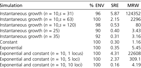
Table 1 Empirical measures of performance in the simulations described in the text
Simulation % ENV SRE MRW
Instantaneous growth (n= 10,s= 31) 96 5.87 124352 Instantaneous growth (n= 10,s= 63) 100 2.15 2296 Instantaneous growth (n= 10,s= 120) 98 0.53 80 Instantaneous growth (n= 25) 90 0.40 3.43 Instantaneous growth (n= 35) 92 0.31 3.16
Constant 100 0.30 1.16
Exponential 100 0.35 5.45
Exponential and constant (n= 10, 1 locus) 100 4.31 22608 Exponential and constant (n= 10, 5 loci) 100 2.37 309.1 Exponential and constant (n= 10, 10 loci) 100 0.16 4.19
Data availability
The methods presented in this article are implemented in the open source R package phylodyn (https://github.com/ JuliaPalacios/phylodyn). The datafiles necessary to repro-duce both the simulated and real data analyses are provided with the R package.
Results
The performance of BESTT in applications to simulated data
We tested our new method, BESTT, on simulated data under four different demographic scenarios. Note that in this section, NðtÞ is rescaled to the coalescent timescale, meaning that 1=NðtÞis the pairwise rate of coalescence at timetin the past relative to the rate at the present time zero. We simulated genealogies under four different population size trajectories:
1. A period of exponential growth followed by constant size:
N tð Þ ¼ 1 if t2 ð0;0:1Þ; exp 1ð 10tÞ if t2 ð0:1;NÞ:
(15)
2. A trajector with instantaneous growth:
N tð Þ ¼ 1 if t2 ð0;0:05Þ; 0:05 if t2 ð0:05;NÞ:
(16)
3. Exponential growth:N tð Þ ¼25e-5t. 4. A constant trajectory:N tð Þ ¼1.
Given a genealogy of length L¼Pnj¼2jðtj2tjþ1Þ, where tj2tjþ1 is the intercoalescent length while there arej line-ages, we drew the total number of mutations (segregating sites)saccording to a Poisson distribution with parametermL. We then placed the mutations uniformly at random along the branches of the genealogy. For each of thesmutations, we assigned the mutant type to individuals descending from the
branch where the mutation occurred and the ancestral type otherwise.
We summarize our posterior inferenceN^ðtÞby the poste-rior median and 95% Bayesian credible intervals (BCIs) after 200 thousand iterations, and thinned every 10 iterations with 100 iterations of burn in. Our initial number of change points forNðtÞwas set to 50 over the time intervalð0;t2Þ, wheret2is the initialized time to the most recent common ancestor; however, over the course of MCMC iterations, this number could increase or decrease according to the posterior distri-bution oft2.
We assess the accuracy and precision of our estimates using the sum of relative errors (SRE)
SRE¼ X
k
i¼1
^NðviÞ2NðviÞ
NðviÞ ;
(17)
whereN^ðviÞis the estimated effective population size trajec-tory at time vi. Second, we computed the mean relative width (MRW) as
MRW¼ X
k
i¼1
^NupðviÞ2N^loðviÞ
k NðviÞ ;
(18)
where Nup^ ðviÞ corresponds to the 97.5% upper limit and
^
NloðviÞcorresponds to the 2.5% lower limit of the estimated posterior distribution ofNðviÞ. In addition, we measured how well the 95% credible intervals cover the truth and compute the envelope measure, ENV:
ENV¼
Pk i¼11
^
NloðviÞ#NðviÞ#N^upðviÞ
k (19)
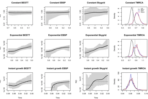
column of Figure 8. Posterior medians and 95% credible inter-vals are shown as black curves and gray shaded areas, respec-tively. The trajectories used to simulate the data are depicted as dashed lines. Figure 8 shows that our BESTT method recovers the constant and exponential growth trajectories very well, but the instantaneous growth scenario is less accurate and with high uncertainty (wide credible intervals). In all three cases, our envelope measure is.95%. Performance measures on all simulations are summarized in Table 1.
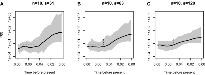
We analyzed the effect of increasing the number of segre-gating sites, the number of samples, and the number of independent genealogies on posterior inference with BESTT. In all three cases, we expect our method to better recover the truth. Figure 5 shows our results on simulated data under a population size trajectory with instantaneous growth (Equa-tion 16) ofn¼10 individuals with 31, 63, and 120 segregat-ing sites. As expected, our method recovers the truth with higher precision (MRW) and accuracy (SRE) when we in-crease the number of segregating sites. Increasing the num-ber of segregating sites may result in more constraints in the gene tree. For n¼10, there are 7936 possible ranked tree shapes; however, for the data sets simulated with 31, 63, and 102 segregating sites, there are only 2582632, 2670634, and 55667 ranked tree shapes compatible with their corre-sponding gene trees. These numbers were estimated by im-portance sampling (Cappello and Palacios 2019).
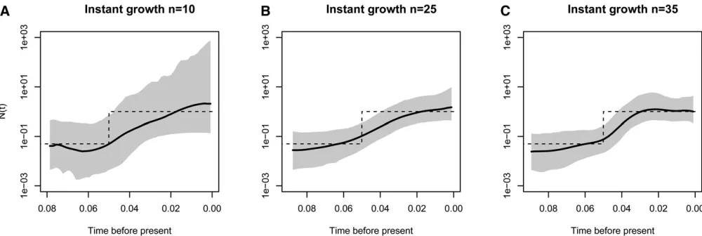
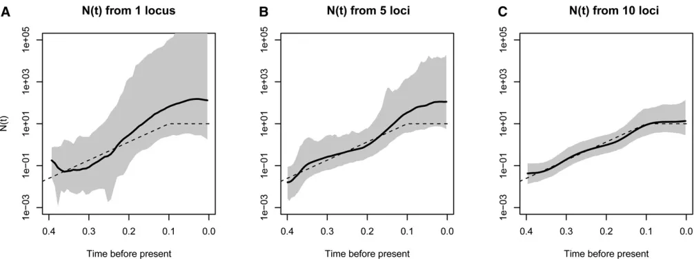
As another performance assessment, we simulated data sets from a population size trajectory with instantaneous growth with varying numbers of samples. We simulated data sets withn¼10, 25, and 35 samples with 215 expected num-bers of segregating sites. Our results depicted in Figure 6 show that our method performs better in terms of SRE and MRE when the number of samples increases. Similarly, pre-cision (MRW) and accuracy (SRE) increases when inference is done from a larger number of independent data sets. Fi-nally, Figure 7 shows our results from 1, 5, and 10 data sets simulated from 1, 5, and 10 independent genealogies of 10
in-dividuals with a population size trajectory of growth followed by a constant period (Equation 15). As expected, our meth-od’s performance substantially increases by increasing the number of independent data sets.
Comparison to other methods
To our knowledge, there is no other method for inferring (variable) effective population size over time from haplotype data that assumes the infinite sites mutation and a nonpara-metric prior onNðtÞ; therefore, we cannot directly compare our method to others. Moreover, our method is the only one that explicitly averages over Tajima genealogies instead of Kingman genealogies. BEAST (Drummond et al.2012) is a program for analyzing molecular sequences that uses MCMC to average over the Kingman tree space and it is therefore a good reference for comparison to our method. We compared our results to the Extended Bayesian Skyline Plot method (EBSP) (Heled and Drummond 2008) and the Skygrid method (Gillet al.2013) implemented in BEAST.
Since the infinite sites mutation model is not implemented in BEAST, wefirst converted our simulated sequences of 0s and 1s to sequences of nucleotides by sampling sancestral nucleotides uniformly on fA;T;C;Gg and assigning one of the remaining three types uniformly at random to be the mutant type. This corresponds to a simulation of the Jukes– Cantor mutation model (Jukes and Cantor 1969) that is cur-rently implemented in BEAST.
We compare the results of BESTT to those of BEAST EBSP and Skygrid (Drummondet al.2005, 2012) in Figure 8. We note that results from BEAST are generated from 10 million iterations and thinned every 1000 iterations, while results from BESTT are generated from 200 thousand iterations.
intervals are uneven with very wide intervals at the ends. In all cases, the BEAST Skygrid results have wider credible in-tervals. For the instantaneous growth simulation (Figure 8, third row), BEAST EBSP did not generate many simulations beyond the time point 0.06; for this reason, we recomputed the performance statistics for the overlapping time interval ð0;0:06Þ. In this interval, BESTT outperforms both methods implemented in BEAST in terms of envelope and SRE. The last column of Figure 8 shows the posterior distribution of the TMRCA. For the case of constant population size, the true value of the TMRCA is contained in the 95% BCI estimated with BESTT but it is not contained in the 95% BCIs estimated with the two methods implemented in BEAST. In the expo-nential growth simulation, the true TMRCA is contained in the 95% BCIs estimated with the three methods and the in-stant growth method; the true TMRCA is not contained in the 95% BCIs of the three methods.
We note that BEAST Bayesian Skygrid (Gillet al.2013) is a more comparable method to BESTT since it assumes Gauss-ian process priors on logNðtÞlike BESTT.
Computational performance of BESTT
BESTT approximates the posterior distribution (a) PrððNðtÞÞt$0;gT;tY;mÞ, wheregT is a Tajima’s genealogy instead of (b) PrððNðtÞÞt$0;g;tY*;mÞ, where gis a King-man’s genealogy and Y* is the labeled data, to estimate ðNðtÞÞt.0. These two posterior distributions are the same when every individual of the sample has its own private mu-tation group and no shared mumu-tation groups. Otherwise, the number of Tajima’s trees compatible with observed dataY, i.e., Tajima’s treesgTsuch that PrðgTYÞ.0, is smaller than the number of Kingman’s trees compatible with observed labeled data Y* (Cappello and Palacios 2019). That is, we are required to estimate the posterior of a smaller number of trees. For this reason, we argue that Tajima’s coalescent is
a more efficient model than Kingman’s coalescent for estimat-ing the posterior distribution ofðNðtÞÞt$0. However, a single conditional likelihood calculation PrYgT;m requires the sum over all possible allocation of mutation groups to branches ofgT. Our algorithm only accounts for allocations constrained by the DAG and the ranked tree shape of gT. For the data depicted in Figure 2, A and B andgTof Figure 2C, there are only eight different possible allocation paths of all mutation groups to branches. In Appendix C, we detail how our algo-rithmfinds these paths. The number of paths depends on the number of subtrees with the same family size path in the DAG and in the ranked tree shape. In the best case, our algorithm willfind a path inOðnoÞ, wherenois the number of nodes in the gene tree. In general, the number of allocation paths will be much smaller than the number of labeled trees compatible with a ranked tree shape. In our implementation, we estimate posterior (a) with MCMC. The main difference between our MCMC algorithm and the MCMC algorithm implemented in BEAST is the tree topology sampler. While our MCMC algo-rithm explores the space of ranked tree shapes with local move proposals of ranked tree shapes, BEAST explores the space of labeled, ranked tree shapes with local move proposals of la-beled trees. A formal assessment of the efficiency of our MCMC algorithm and its comparison to the MCMC implementation in BEAST is beyond the scope of this manuscript and subject of future research.
Inferring human population demography from mtDNA
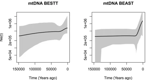
with the infinite sites mutation model. Thefinalfile is available inhttps://github.com/JuliaPalacios/phylodyn. To encode our data as 0s and 1s, we use the inferred root sequenceRSRSof Beharet al.(2012) to define the ancestral type at each site. To rescale our results in units of years, we assumed a mutation rate per site per year of 1:331028 (Rebolledo-Jaramillo et al. 2014). We compare our results with the Extended Bayesian Skyline method (Drummond et al. 2012) implemented in BEAST in Figure 9. When applying BEAST, we assumed the Jukes–Cantor mutation model. Both methods detect an infl ec-tion point20 KYA followed by exponential growth. The mean TMRCA inferred for these YRI mtDNA samples with BESTT is 170 KYA with a 95% BCI of 142ð ;868; 207;455Þ, while the mean TMRCA inferred with BEAST is160 KYA with a 95% BCI of 133ð ;239; 196;900Þ. In Appendix D, we include two more comparisons of BESTT and BEAST.
Discussion
The size of emergent sequencing data sets prohibits the use of standard coalescent modeling for inferring evolutionary
parameters. The main computational bottleneck of coalescent-based inference of evolutionary histories lies in the large cardinality of the hidden state space of genealogies. In the standard Kingman coalescent, a genealogy is a random la-beled bifurcating tree that models the set of ancestral rela-tionships of the samples. The genealogy accounts for the correlated structure induced by the shared past history of organisms and explicit modeling of genealogies is fundamen-tal for learning about the past history of organisms. However, the genomic era is producing large data sets that require more efficient approaches that efficiently integrate over the hidden state space of genealogies.
In this manuscript, we show that a lower-resolution co-alescent model on genealogies, Tajima’s coco-alescent, can be used as an alternative to the standard Kingman coalescent model. In particular, we show that the Tajima coalescent model provides a feasible alternative that integrates over a smaller state space than the standard Kingman model. The main advantage in Tajima’s coalescent is modeling of the ranked tree topology as opposed to the fully labeled tree topology, as in Kingman’s coalescent.
A priori, the cardinality of the state space of ranked tree shapes is much smaller than the cardinality of the state space of labeled trees. However, in this manuscript we show that when the Tajima coalescent model is coupled with the infi n-ite sn-ites mutation model, the space of ranked tree shapes is constrained by the data and the reduction on the cardinality of the hidden state space of Tajima’s trees is even more pro-nounced than expected.
To leverage the constraints imposed by the data and the infinite sites mutation model, we apply Dan Gusfield’s perfect phylogeny algorithm (Gusfield 1991) to represent sequence alignments as a gene tree. We exploit the gene tree represen-tation for conditional likelihood calculations and for explor-ing the state space of ranked tree shapes.
For the calculation of the likelihood of the data conditioned on a given Tajima’s genealogy, we augment the gene tree representation of the data with the Tajima’s genealogy and map observed mutations to branches. We define a DAG with the augmented gene tree. This new representation as a DAG allows for calculating the likelihood as a backtracking algo-rithm that transverses the gene tree from the leaves to the root. Our implementation’s computational bottleneck lies in the likelihood calculation. Given a Tajima’s genealogy, our likelihood algorithm sums over all possible allocations of mu-tation groups to branches. Although this number is generally much smaller than the number of labeled genealogies, our algorithm can be further optimized. In future studies, we will explore a sum-product type of algorithm for the likelihood
calculation. In the present implementation, we are able to infer effective population size trajectories from samples of size n35 on a regular personal laptop computer within few hours.
Our statistical framework draws on Bayesian nonparamet-rics. We place aflexible geometric random walk process prior on the effective population size that allows us to recover population size trajectories with abrupt changes in simula-tions. The inference procedure proposed in this manuscript relies on MCMC methods with three large Gibbs block updates of: coalescent times, effective population size trajectory, and ranked tree shape topology. We use Hamiltonian Monte Carlo updates for continuous random variables—coalescent times and effective population size—and a Metropolis–Hastings sampler for exploring the space of ranked tree shapes. For exploring the genealogical space, Markovtsovaet al.(2000) suggest a joint local proposal for both coalescent times and topology. Here, we restrict our attention to the topology alone. A future line of research includes the development of a joint local proposal of coalescent times and ranked tree shapes. We also envision that a joint sampler of coalescent times and effective population size trajectories should im-prove mixing and convergence.
Our method does not model recombination, population structure, or selection. It assumes completely linked and neutral segments from individuals from a single population, and the infinite sites mutation model. While this model is a good approximation for some human molecular data, it is not appropriate for modeling molecular data from other organ-isms such as pathogens and viral populations. Finally, haplo-type data of many organisms are usually sparse with few unique haplotypes presented at high frequencies. Since our algorithm exploits molecular data at the haplotype level, our proposed method is ideally suited for this scenario where the space of ranked tree shapes is drastically smaller than the space of labeled topologies.
Acknowledgments
We acknowledge the developers of R-ape, R-phangorn, and R-phylodyn, which facilitated our implementations, and thank the editor and two anonymous referees whose suggestions considerably improved the manuscript. This research was supported in part by National Institutes of Health grant R01 GM-131404 and funding from the Alfred P. Sloan Foundation to J.A.P, and by National Science Foundation CAREER award DBI-1452622 to S.R. A.V. was Table 2 Performance comparison between BESTT and BEAST in simulations
% ENV SRE MRW
Simulation BESTT EBSP Skygrid BESTT EBSP Skygrid BESTT EBSP Skygrid
Constant 100 100 100 0.30 0.24 0.24 1.16 1.49 4.41
Exponential 100 97 100 0.35 0.26 0.29 5.45 2.56 46.13
Inst. growth 97 94 100 0.61 2.65 22.60 105.60 14.95 .1000
BESTT, Bayesian Estimation of population size changes by Sampling Tajima’s Trees; % ENV, % envelope measure; EBSP, Extended Bayesian Skyline Plot; MRW, mean relative width; SRE, sum of relative errors. Bold values indicate best performance.
supported in part by the Chaire Modélisation Mathématique et Biodiversité program of VEOLIA Environnement, École Polytechnique, Museum National d’Histoire Naturelle, Fon-dation X. A.V. and J.A.P. were supported by the France-Stanford Center for Interdisciplinary Studies.
Literature Cited
1000 Genomes Project Consortium, Auton, A., G. R. Abecasis, D. M. Altshuler, R. M. Durbin et al., 2015 A global reference for human genetic variation. Nature 526: 68–74.https://doi.org/ 10.1038/nature15393
Aberer, A. J., A. Stamatakis, and F. Ronquist, 2016 An efficient independence sampler for updating branches in Bayesian Mar-kov chain Monte Carlo sampling of phylogenetic trees. Syst. Biol. 65: 161–176.https://doi.org/10.1093/sysbio/syv051
Anderson, S., A. T. Bankier, B. G. Barrell, M. H. de Bruijn, A. R. Coulsonet al., 1981 Sequence and organization of the human mitochondrial genome. Nature 290: 457–465.https://doi.org/ 10.1038/290457a0
Andrews, R. M., I. Kubacka, P. F. Chinnery, R. N. Lightowlers, D. M. Turnbullet al., 1999 Reanalysis and revision of the Cambridge reference sequence for human mitochondrial DNA. Nat. Genet. 23: 147.https://doi.org/10.1038/13779
Behar, D. M., M. Van Oven, S. Rosset, M. Metspalu, E.-L. Loogväli
et al., 2012 A“Copernican”reassessment of the human mito-chondrial DNA tree from its root. Am. J. Hum. Genet. 90: 675– 684.https://doi.org/10.1016/j.ajhg.2012.03.002
Bhaskar, A., Y. R. Wang, and Y. S. Song, 2015 Efficient inference of population size histories and locus-specific mutation rates from large-sample genomic variation data. Genome Res. 25: 268–279.https://doi.org/10.1101/gr.178756.114
Cappello, L., and J. A. Palacios, 2019 Sequential importance sam-pling for multi-resolution Kingman-Tajima coalescent counting. arXiv. Available at:https://arxiv.org/abs/1902.05527.
Disanto, F., and T. Wiehe, 2013 Exact enumeration of cherries and pitchforks in ranked trees under the coalescent model. Math. Biosci. 242: 195–200. https://doi.org/10.1016/j.mbs. 2013.01.010
Donnelly, P., and S. Tavaré, 1995 Coalescents and genealogical structure under neutrality. Annu. Rev. Genet. 29: 401–421.
https://doi.org/10.1146/annurev.ge.29.120195.002153
Drummond, A., and A. Rodrigo, 2000 Reconstructing genealo-gies of serial samples under the assumption of a molecu-lar clock using serial-sample UPGMA. Mol. Biol. Evol. 17: 1807–1815. https://doi.org/10.1093/oxfordjournals.molbev. a026281
Drummond, A. J., A. Rambaut, B. Shapiro, and O. G. Pybus, 2005 Bayesian coalescent inference of past population dynam-ics from molecular sequences. Mol. Biol. Evol. 22: 1185–1192.
https://doi.org/10.1093/molbev/msi103
Drummond, A. J., M. A. Suchard, D. Xie, and A. Rambaut, 2012 Bayesian phylogenetics with BEAUti and the BEAST 1.7. Mol. Biol. Evol. 29: 1969–1973.https://doi.org/10.1093/ molbev/mss075
Gill, M. S., P. Lemey, N. R. Faria, A. Rambaut, B. Shapiroet al., 2013 Improving Bayesian population dynamics inference: a coalescent-based model for multiple loci. Mol. Biol. Evol. 30: 713–724.https://doi.org/10.1093/molbev/mss265
Griffiths, R. C., and S. Tavaré, 1994a Simulating probability dis-tributions in the coalescent. Theor. Popul. Biol. 46: 131–159.
https://doi.org/10.1006/tpbi.1994.1023
Griffiths, R. C., and S. Tavaré, 1994b Sampling theory for neu-tral alleles in a varying environment. Philos. Trans. R. Soc.
Lond. B Biol. Sci. 344: 403–410. https://doi.org/10.1098/ rstb.1994.0079
Griffiths, R. C., and S. Tavaré, 1995 Unrooted genealogical tree probabilities in the infinitely-many-sites model. Math. Biosci. 127: 77–98.https://doi.org/10.1016/0025-5564(94)00044-Z
Griffiths, R. C., and S. Tavaré, 1996 Monte Carlo inference meth-ods in population genetics. Math. Comput. Model. 23: 141–158.
https://doi.org/10.1016/0895-7177(96)00046-5
Gronau, I., M. J. Hubisz, B. Gulko, C. G. Danko, and A. Siepel, 2011 Bayesian inference of ancient human demography from individual genome sequences. Nat. Genet. 43: 1031–1034.
https://doi.org/10.1038/ng.937
Gusfield, D., 1991 Efficient algorithms for inferring evolution-ary trees. Networks 21: 19–28. https://doi.org/10.1002/ net.3230210104
Heled, J., and A. J. Drummond, 2008 Bayesian inference of pop-ulation size history from multiple loci. BMC Evol. Biol. 8: 289.
https://doi.org/10.1186/1471-2148-8-289
Hobolth, A., M. K. Uyenoyama, and C. Wiuf, 2008 Importance sampling for the infinite sites model. Stat. Appl. Genet. Mol. Biol. 7: Article32.https://doi.org/10.2202/1544-6115.1400
Jukes, T. H., and R. C. Cantor, 1969 Evolution of protein mole-cules, pp. 21–132 inMammalian Protein Metabolism, edited by H. N. Munro. Academic Press, New York. https://doi.org/ 10.1016/B978-1-4832-3211-9.50009-7
Karcher, M. D., J. A. Palacios, S. Lan, and V. N. Minin, 2017 phylodyn: an r package for phylodynamic simulation and inference. Mol. Ecol. Resour. 17: 96–100.https://doi.org/ 10.1111/1755-0998.12630
Kingman, J., 1982a The coalescent. Stochastic Process. Appl. 13: 235–248.https://doi.org/10.1016/0304-4149(82)90011-4
Kingman, J. F. C., 1982b Exchangeability and the evolution of large populations, pp. 97–112 in Exchangeability in Probability and Statistics, edited by G. Koch and F. Spizzichino. North-Hol-land, Amsterdam.
Kuhner, M. K., 2006 LAMARC 2.0: maximum likelihood and Bayesian estimation of population parameters. Bioinformatics 22: 768–770.https://doi.org/10.1093/bioinformatics/btk051
Kuhner, M. K., and L. Smith, 2007 Comparing likelihood and Bayesian coalescent estimation of population parameters. Genetics 175: 155–165. https://doi.org/10.1534/genet-ics.106.056457
Kuhner, M. K., J. Yamato, and J. Felsenstein, 1998 Maximum likelihood estimation of population growth rates based on the coalescent. Genetics 149: 429–434.
Lan, S., J. A. Palacios, M. Karcher, V. Minin, and B. Shahbaba, 2015 An efficient Bayesian inference framework for coales-cent-based nonparametric phylodynamics. Bioinformatics 31: 3282–3289.https://doi.org/10.1093/bioinformatics/btv378
Li, H., and R. Durbin, 2011 Inference of human population history from individual whole-genome sequences. Nature 475: 493– 496.https://doi.org/10.1038/nature10231
Markovtsova, L., P. Marjoram, and S. Tavaré, 2000 The age of a unique event polymorphism. Genetics 156: 401–409.
Minin, V. N., E. W. Bloomquist, and M. A. Suchard, 2008 Smooth skyride through a rough skyline: Bayesian coalescent-based in-ference of population dynamics. Mol. Biol. Evol. 25: 1459–1471.
https://doi.org/10.1093/molbev/msn090
Neal, R. M., 2011 MCMC using Hamiltonian dynamics, pp.113– 162 in Handbook of Markov Chain Monte Carlo, edited by S. Brooks, A. Gelman, G. L. Jones, and X.-L. Meng. CRC Press, Boca Raton, FL.
Palacios, J. A., and V. N. Minin, 2013 Gaussian process-based Bayesian nonparametric inference of population size trajectories from gene genealogies. Biometrics 69: 8–18. https://doi.org/ 10.1111/biom.12003
Palacios, J. A., J. Wakeley, and S. Ramachandran, 2015 Bayesian nonparametric inference of population size changes from se-quential genealogies. Genetics 201: 281–304.https://doi.org/ 10.1534/genetics.115.177980
Rannala, B., and Z. Yang, 2003 Bayes estimation of species di-vergence times and ancestral population sizes using DNA se-quences from multiple loci. Genetics 164: 1645–1656. Rasmussen, C. E., and C. K. I. Williams, 2006 Gaussian Processes
for Machine Learning. MIT Press, Cambridge, MA.
Rebolledo-Jaramillo, B., M. S. Su, N. Stoler, J. A. McElhoe, B. Dick-inset al., 2014 Maternal age effect and severe germ-line bot-tleneck in the inheritance of human mitochondrial DNA. Proc. Natl. Acad. Sci. USA 111: 15474–15479. https://doi.org/ 10.1073/pnas.1409328111
Sainudiin, R., K. Thornton, J. Harlow, J. Booth, M. Stillmanet al., 2011 Experiments with the site frequency spectrum. Bull. Math. Biol. 73: 829–872. https://doi.org/10.1007/s11538-010-9605-5
Sainudiin, R., T. Stadler, and A. Véber, 2015 Finding the best resolution for the Kingman-Tajima coalescent: theory and appli-cations. J. Math. Biol. 70: 1207–1247.https://doi.org/10.1007/ s00285-014-0796-5
Schiffels, S., and R. Durbin, 2014 Inferring human population size and separation history from multiple genome sequences. Nat. Genet. 46: 919–925.https://doi.org/10.1038/ng.3015
Schliep, K. P., 2011 phangorn: phylogenetic analysis in R. Bioin-formatics 27: 592–593.https://doi.org/10.1093/bioinformatics/ btq706
Sheehan, S., K. Harris, and Y. S. Song, 2013 Estimating variable effective population sizes from multiple genomes: a sequentially Markov conditional sampling distribution approach. Genetics 194: 647–662.https://doi.org/10.1534/genetics.112.149096
Slatkin, M., and R. Hudson, 1991 Pairwise comparisons of mito-chondrial DNA sequences in stable and exponentially growing populations. Genetics 129: 555–562.
Stephens, M., and P. Donnelly, 2000 Inference in molecular pop-ulation genetics. J. R. Stat. Soc. Series B Stat. Methodol. 62: 605–635.https://doi.org/10.1111/1467-9868.00254
Tajima, F., 1983 Evolutionary relationship of DNA sequences in
finite populations. Genetics 105: 437–460.
Tavaré, S., (2004). Part I: ancestral inference in population genet-ics, pp 1–188 in Lectures on Probability Theory and Statistics,
Volume 1837 of Lecture Notes in Mathematics. Springer-Verlag, New York.
Terhorst, J., J. A. Kamm, and Y. S. Song, 2017 Robust and scal-able inference of population history from hundreds of unphased whole genomes. Nat. Genet. 49: 303–309. https://doi.org/ 10.1038/ng.3748
Watterson, G., 1975 On the number of segregating sites in genet-ical models without recombination. Theor. Popul. Biol. 7: 256– 276.https://doi.org/10.1016/0040-5809(75)90020-9
Whidden, C., and F. A. Matsen, IV, 2015 Quantifying MCMC ex-ploration of phylogenetic tree space. Syst. Biol. 64: 472–491.
https://doi.org/10.1093/sysbio/syv006
Wu, Y., 2010 Exact computation of coalescent likelihood for pan-mictic and subdivided populations under the infinite sites model. IEEE/ACM Trans. Comput. Biol. Bioinformatics 7: 611– 618.https://doi.org/10.1109/TCBB.2010.2
Appendix
Appendix A: Matrix Representation of a Ranked Tree Shape
Our algorithms exploit the following encoding of a ranked tree shape by a triangular matrix of sizen3n, which we denote byF
(Figure A1). Recall that, by convention,tnþ1 ¼0 andt1¼ þN. First, we declare thatFi;j¼0 ifj.i. Next, the number of lineages through time is encoded on the diagonal ofF:Fi;i¼i foriinf2;3;. . .;ng. Finally, forj,i, the entryFi;jdenotes the number of lineages that do not coalesce in the time interval ðtiþ1;tjÞ; in particular,Fi;1¼0 and for everyiinf2;3;. . .;ng,
Fn;idenotes the number of singletons (i.e., external branches that have not coalesced) in the time intervalðtiþ1;tiÞ(Figure A1). Other statistics of the ranked tree shape can be expressed in terms of the corresponding matrixF. Among them, the num-bercof cherries is equal to the number of times that the num-ber of singletons decreases by two between linesiandi21, since such an event means that the coalescence separating these two epochs was that of two external branches. That is,
c¼X
n
i¼3
1fFn;i2Fn;i21¼2g:
Appendix B
Detailed allocation of mutation groups alonggT
The latent allocation random variablesfAjgare constrained by the information in the Tajima’s genealogy gT. In a givengT, every subtree is labeled by its ranking from past to present (Figure A1). Subtreeiis subtended by branchbi with length li, fori¼2;. . .;n. We will assume thatl2, the length of the root branch, is 0. Letcbe the number of cherries (nodes with two leaves) ingT; the two branches of a given cherry share the same label bj2 fbnþ1;. . .;bnþcg. The actual label of external branches is arbitrary but, for ease of exposition in ourfigures, we first label the cherries’ branches from left to right by fbnþ1;. . .;bnþcg; singleton branches are labeled from left to right by bnþcþ1;. . .;b2n2c (Figure 2C). As mentioned before, the length ofXjis the number of the corresponding sister nodes inT that were grouped together in forming nodeZj. In this case, Aj¼ ðAj;1;. . .;Aj;jchðjÞjÞdenotes a collection ofjchðjÞjvectors of
branch labels ingTsubtending the child node subtrees of node Zj.Aj;1corresponds to the branch subtending from the leftmost child node ofZjonD,Aj;2corresponds to the branch subtending from the next child node ofZj, etc., andAj;jchðjÞjcorresponds to the branch subtending from the rightmost child node ofZjonD. Observe that, since we group some of the leaf nodes inT into a single node inD, anyAj;kmay be a vector of branch labels; for exampleA1;1¼ ðb12;b9ÞandA1;2¼b10in Figure 3B.
Appendix C
Algorithms for conditional likelihood calculation
The following two algorithms detail the calculation of PrðYgT;mÞ
.Yis encoded inGeneTree, the observed data
as a tree structure. Each node in GeneTreehas number of descendants (or lineages) and mutation information at-tached to it. Tajima’s genealogy gT is encoded as Fpath, which contains the ranked tree shapeFn, andtimes, which contains the vector of coalescent timestmultiplied by the mutation ratem.
Algorithm 1 Calculate LikelihoodðFpath;times;GeneTreeÞ procedure
Input:GeneTree,FPath
Output:Log LikelihoodLL
1: Initiatepoolto be the set of leaf nodes ofGeneTreewith at least one descendant. InitiateLLandindexto be zero. Initiatecurrent_ pathto be empty.
2: Call CalcLL_recursive(LL, index, current_path, Fpath, times, Genetree).
3:returnLL
Algorithm 2 CalcLL_recursive(LL, index, current_ path,
Fpath,times,Genetree) procedure
1:if index¼lenðpathÞ {When a complete path node is
found} then
2: fornodeintreedo
3: Calculate log likelihood based ontimesand number of mutations ofnodeincurrent_ path.
4: Accumulate to total log likelihoodLL
5: end for
6:else
7: fornodeinpooldo
8: Check compatibility of thenode, according to the givenFpath.
9: ifnodeis compatible withFpaththen
10: Updatenodeby assigning it to the current step in Fpath
11: Updatepool. If anodehas been mapped entirely, removenode from pool, update its parentnode, and potentially add parent node topoolif parent node has not been entirely assigned.
12: Append thisnodetocurrent_ path
13: Call CalcLL_recursive(LL, index11,current_path, Fpath, Genetree)
14: Restore previousnode,pool, andcurrent_ path
15: end if
16: end for
17:end if
To illustrate algorithms 1 and 2, we use our examples of Figure 2 and Figure 3. Algorithm 1 initiates the pool with nodes Z3;Z4;Z6;Z8;Z10. Then, Algorithm 2 cycles through this list. Assume thefirst node isZ8. This node hasd8 ¼2 descendants
![Figure 2 Data structures employed by our method, Bayesian Estimation of population size changes by Sampling Tajimawith the same label in (A)]](https://thumb-us.123doks.com/thumbv2/123dok_us/1505305.1184296/4.603.90.516.56.490/figure-structures-employed-bayesian-estimation-population-sampling-tajimawith.webp)