Improved Batching for Confidence Interval Construction in Steady-State Simulation

(1)

Abstract

STEIGER, NATALIE MILLER. Improved Batching for Confidence Interval Con-struction in Steady-State Simulation. (Under the direction of James R. Wilson.)

(2)

(3)

Biography

Natalie Miller Steiger was born on September 18, 1950 in Vicksburg, MS. She gradu-ated from St. Francis Xavier Academy in 1968. She was a member of the University Honors Program at the University of Southern Mississippi in Hattiesburg, MS where she earned B.S. (1972) and M.S. (1973) degrees in Mathematics.

In 1973, she was employed as a Junior Engineer for South Central Bell in Jack-son, MS. In 1975, she began work for Cities Service Oil and Gas Company in Tulsa, OK. She held various positions as analyst and manager while at Cities Service and remained with the company through its acquisition by Occidental Petroleum Com-pany. In 1979, she married David Steiger. She resigned from Occidental Petroleum Company in 1986 to be a full-time mother to Rebecca, who was born in November, 1985. Her son, Benjamin, was born in January, 1988.

(4)

Acknowledgments

I thank Dr. James R. Wilson, Chair of my advisory committee, for the considerable effort he expended and the extreme patience he displayed in guiding me through this research and the composition of this dissertation. His dedication to doing the job well is truly inspiring. I thank Drs. Steve Roberts, Yahya Fathi, and Len Stefanski for serving as advisors on my committee and for their constructive input. I also thank Dr. Jack Silverstein for serving as the graduate representative on my committee. I thank Dr. Jeff Joines for his assistance with programming and computer problems.

(5)

List of Tables

5.1 Steady-State Expected Waiting Time in Selected Queueing Systems . 113 5.2 Parameters for the Selected Central Server Models . . . 115 5.3 Performance of Batch-Means Procedures for the 2-State DTMC with

Alternating Correlation Structure as Defined by (3.65) and (3.66) Based on 100 Independent Replications of Nominal 90% Confidence Intervals 117 5.4 Performance of Batch-Means Procedures for the 2-State DTMC with

High Positive Correlation Structure as Defined by (3.66) and (3.67) Based on 100 Independent Replications of Nominal 90% Confidence Intervals . . . 118 5.5 Performance of Batch-Means Procedures for the 8-State DTMC as

De-fined by (3.68) and (3.69) Based on 100 Independent Replications of Nominal 90% Confidence Intervals . . . 119 5.6 Performance of Batch-Means Procedures for the AR(1) Process (3.75)

with ϕ= 0.9 and µX = 2.0 Based on 100 Independent Replications of

Nominal 90% Confidence Intervals . . . 120 5.7 Performance of Batch-Means Procedures for the EAR(1) Process (3.78)

with ϕ= 0.9 and µX = 2.0 Based on 100 Independent Replications of

Nominal 90% Confidence Intervals . . . 121 5.8 Performance of Batch-Means Procedures for the M/M/1 Queue

Wait-ing Time Process withτ = 0.9 Based on 100 Independent Replications of Nominal 90% Confidence Intervals . . . 122 5.9 Performance of Batch-Means Procedures for the M/M/1 Queue

Wait-ing Time Process withτ = 0.8 Based on 100 Independent Replications of Nominal 90% Confidence Intervals . . . 124 5.11 Performance of Batch-Means Procedures for the M/M/1 LIFO Queue

Waiting Time Process with τ = 0.8 Based on 100 Independent Repli-cations of Nominal 90% Confidence Intervals . . . 125 5.12 Performance of Batch-Means Procedures for the M/M/1 SIRO Queue

(8)

5.13 Performance of Batch-Means Procedures for the E4/M/1 Queue

Wait-ing Time Process withτ = 0.8 Based on 100 Independent Replications of Nominal 90% Confidence Intervals . . . 127 5.14 Performance of Batch-Means Procedures for the M/H2/1 Queue

Wait-ing Time Process withτ = 0.8 Based on 100 Independent Replications of Nominal 90% Confidence Intervals . . . 129 5.16 Performance of Batch-Means Procedures for the M/M/1/M/1 Queue

Waiting Time Process with τ = 0.8 Based on 100 Independent Repli-cations of Nominal 90% Confidence Intervals . . . 130 5.17 Performance of Batch-Means Procedures for the Time-Shared Model

Based on 100 Independent Replications of Nominal 90% Confidence Intervals . . . 131 5.18 Performance of Batch-Means Procedures for the Central Server Model

1 Based on 100 Independent Replications of Nominal 90% Confidence Intervals . . . 132 5.19 Performance of Batch-Means Procedures for the Central Server Model

2 Based on 100 Independent Replications of Nominal 90% Confidence Intervals . . . 133 5.20 Performance of Batch-Means Procedures for the Central Model 3 Based

on 100 Independent Replications of Nominal 90% Confidence Intervals 134 5.21 Performance of Batch-Means Procedures for the Central Server Model

4 Based on 100 Independent Replications of Nominal 90% Confidence Intervals . . . 135 5.22 Performance of Batch-Means Procedures for the (s, S) Inventory

Sys-tem Based on 100 Independent Replications of Nominal 90% Confi-dence Intervals . . . 136 5.23 Performance of LBATCH and ABATCH Algorithms under a Relative

Precision Requirement for 2-state DTMC with High Correlation as Defined by (3.66) and (3.67) Based on 100 Independent Replications of Nominal 90% Confidence Intervals . . . 137 5.24 Performance of LBATCH and ABATCH Algorithms under a Relative

(9)

List of Figures

2.1 Fishman’s Fixed Sample Size Algorithm for Determining Batch Sizem and Number of Batchesk. . . 24 2.2 Law and Carson’s Sequential Algorithm for Determining Batch Sizem

and Number of Batchesk. . . 28 2.3 LBATCH Algorithm for Determining Batch Size m and

Number of Batches k. . . 31 2.4 ABATCH Algorithm for Determining Batch Size m and

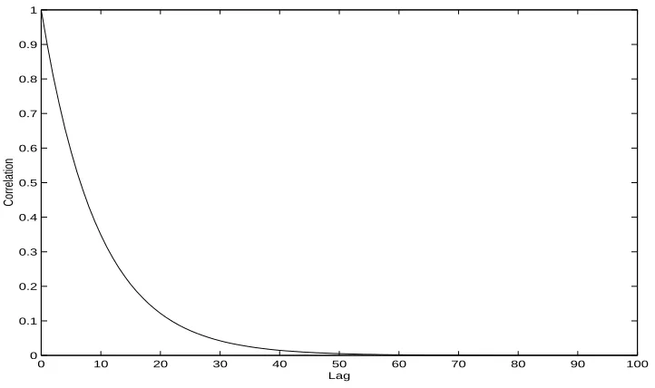
and Number of Batchesk. . . 32 2.5 Nakayama’s Absolute Half-length Two-stage Stopping Procedure . . . 33 2.6 Nakayama’s Relative Half-length Two-stage Stopping Procedure . . . 34 3.1 Lag-q Correlation Corr(Ni, Ni+q) of Observations of Cost Function

Ni = η(Xi) on 2-State DTMC with Alternating Correlation

Struc-ture as Defined by (3.65) and (3.66). The SSVC σ2 = 2.083 and σ2

N ≡Var[Ni] = 6.25. . . 51

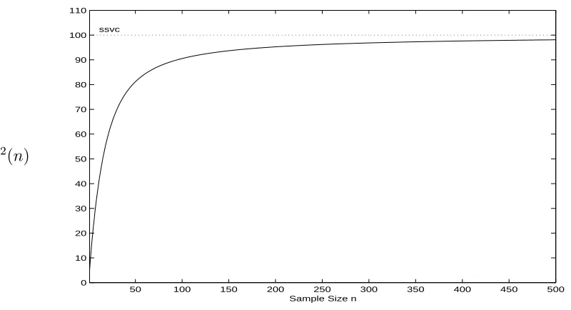
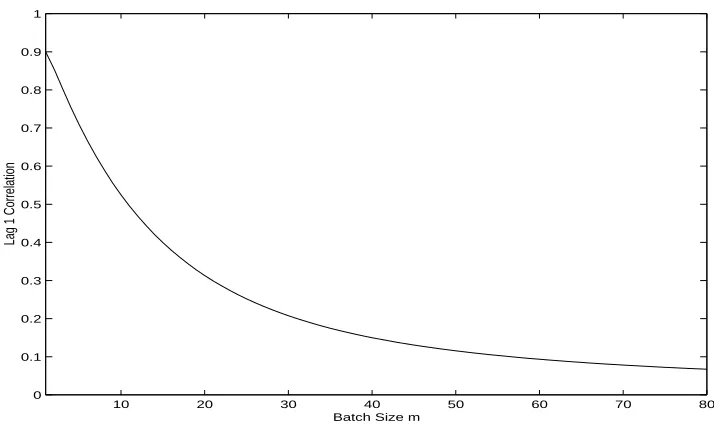
3.2 Lag 1 Correlation of the Batch Means with Batches of Size m for the 2-State DTMC with Alternating Correlation Structure as Defined by (3.65) and (3.66) . . . 51 3.3 σ2_{(n) =} _{nVar[X(n)] for Samples of Size} _n _{for the Cost Function on}

2-State DTMC with Alternating Correlation Structure as Defined by (3.65) and (3.66). The SSVC σ2 _{= 2.083. . . .} ₅₂

3.4 Condition (3.34) on RatiokVar[X(n)]/Var[X(m)] for the 2-State DTMC with Alternating Correlation Structure as Defined by (3.65) and (3.66) for k= 30 Batches of Size m. . . 52 3.5 Condition (3.35) on Ratio E[S2

n,k]/Var[X(m)] for 2-State DTMC with

Alternating Correlation Structure as Defined by (3.65) and (3.66) for k= 30 Batches of Size m. . . 53 3.6 Condition (3.36) on Ratio Var[S2

n,k]/Var

2_{[X(m)] for the 2-State DTMC}

with Alternating Correlation Structure as Defined by (3.65) and (3.66) for k= 30 Batches of Size m. . . 53 3.7 Condition (3.37) on Coefficient of Variation qVar[S2

n,k]/E[Sn,k2 ] for

(10)

3.8 Lag-q Correlation Corr(Ni, Ni+q) of Observations of Cost Function

Ni = η(Xi) on 2-State DTMC with High Positive Correlation as

De-fined by (3.66) and (3.67). The SSVCσ2 _{= 618.75 and}_σ2

N ≡Var[Ni] =

6.25. . . 55 3.9 Lag 1 Correlation of the Batch Means with Batches of Size m for the

2-State DTMC with High Positive Correlation as Defined by (3.66) and (3.67). . . 55 3.10 σ2_{(n) =}_{nVar[X(n)] for Samples of Size} _n _{for the Cost Function on 2}

State DTMC with High Positive Correlation Structure as Defined by (3.66) and (3.67). The SSVC σ2 = 618.75. . . 56 3.11 Condition (3.34) on RatiokVar[X(n)]/Var[X(m)] for the 2-State DTMC

with High Positive Correlation as Defined by (3.66) and (3.67) for k= 30 Batches of Size m. . . 56 3.12 Condition (3.35) on Ratio E[S2

n,k]/Var[X(m)] for 2-State DTMC with

High Positive Correlation as Defined by (3.66) and (3.67) for k = 30 Batches of Sizem. . . 57 3.13 Condition (3.36) on Ratio Var[S2

n,k]/Var

2_{[X(m)] for the 2-State DTMC}

with High Positive Correlation as Defined by (3.66) and (3.67) for k= 30 Batches of Size m. . . 57 3.14 Condition (3.37) on Coefficient of Variation qVar[S2

n,k]/E[Sn,k2 ] for

2-State DTMC with High Positive Correlation Structure as Defined by (3.66) and (3.67) fork = 30 Batches of Size m. . . 58 3.15 Lag-q Correlation Corr(Ni, Ni+q) of Observations of Cost Function

Ni = η(Xi) on 8-State DTMC with Damped Sinusoidal Correlation

as Defined by (3.68) and (3.69). The SSVC σ2 _{= 77.5 and} _σ2

N ≡

Var[Ni] = 132.2. . . 59

3.16 Lag 1 Correlation of the Batch Means with Batches of Sizemfor the 8-State DTMC with Damped Sinusoidal Correlation as Defined by (3.68) and (3.69). . . 59 3.17 σ2(n) =nVar[X(n)] for Samples of Size nfor the Cost Function on

8-State DTMC with Damped Sinusoidal Correlation as Defined by (3.68) and (3.69). The SSVCσ2 _{= 77.5. . . .} ₆₀

3.18 Condition (3.34) on RatiokVar[X(n)]/Var[X(m)] for the 8-State DTMC with Damped Sinusoidal Correlation as Defined by (3.68) and (3.69) for k= 30 Batches of Size m. . . 60 3.19 Condition (3.35) on Ratio E[Sn,k2 ]/Var[X(m)] for 8-State DTMC with

Damped Sinusoidal Correlation as Defined by (3.68) and (3.69) for k= 30 Batches of Size m. . . 61 3.20 Condition (3.36) on Ratio Var[Sn,k2 ]/Var

2

(11)

3.21 Condition (3.37) on Coefficient of Variation qVar[S2

n,k]/E[Sn,k2 ] for

8-State DTMC with Damped Sinusoidal Correlation as Defined by (3.68) and (3.69) fork = 30 Batches of Size m. . . 62 3.22 Lag-q Correlation Corr(Xi, Xi+q) of Wait Times in the M/M/1 Queue

with Utilization τ = 0.9. The SSVC σ2 _{= 37440 and}_σ2

X = 99. . . 64

3.23 Lag 1 Correlation of the Batch Means with Batches of Size m for the Wait Times in the M/M/1 Queue with Utilizationτ = 0.9. . . 64 3.24 σ2_{(n) =}_{nVar[X(n)] for Samples of Size}_n_{of Wait Times in the M/M/1}

Queue with Utilization τ = 0.9. The SSVC σ2 _{= 37440. . . .} ₆₅

3.25 Condition (3.34) on Ratio kVar[X(n)]/Var[X(m)] for Wait Times in the M/M/1 Queue with Utilization τ = 0.9 for k = 30 Batches of Size m. . . 65 3.26 Condition (3.35) on Ratio E[Sn,k2 ]/Var[X(m)] for Wait Times in the

M/M/1 Queue with Utilization τ = 0.9 fork = 30 Batches of Size m. 66 3.27 Condition (3.36) on Ratio Var[S2

n,k]/Var

2_{[X(m)] for the M/M/1 Queue}

Wait Time Process where Utilization τ = 0.9 for k = 30 Batches of Size m. . . 66 3.28 Condition (3.37) on Coefficient of VariationqVar[S2

n,k]/E[Sn,k2 ] for the

M/M/1 Queue Wait Time Process where Utilizationτ = 0.9 fork = 30 Batches of Sizem. . . 67 3.29 Lag-q Correlation Corr(Xi, Xi+q) of Observations of an AR(1) Process

(3.75) with ϕ= 0.9. The SSVC σ2 _{= 100 and} _σ2

X = 5.26. . . 68

3.30 Lag 1 Correlation of the Batch Means with Batches of Size m for an AR(1) Process (3.75) withϕ= 0.9. . . 69 3.31 σ2_{(n) =}_{nVar[X(n)] for Samples of Size} _n_{for an AR(1) Process (3.75)}

with ϕ= 0.9. The SSVC σ2 _{= 100. . . .} ₆₉

3.32 Condition (3.34) on RatiokVar[X(n)]/Var[X(m)] for an AR(1) Process (3.75) with ϕ= 0.9 for k= 30 and Batches Size m. . . 70 3.33 Condition (3.35) Ratio E[Sn,k2 ]/Var[X(m)] for an AR(1) Process (3.75)

with ϕ= 0.9 fork = 30 Batches of Sizem. . . 70 3.34 Condition (3.36) on Ratio Var[S2

n,k]/Var

2_{[X(m)] for an AR(1) Process}

(3.75) with ϕ= 0.9 for k= 30 Batches of Size m. . . 71 3.35 Condition (3.37) on Coefficient of Variation,qVar[S2

n,k]/E[Sn,k2 ], for an

AR(1) Process (3.75) withϕ= 0.9 fork = 30 Batches of Size m. . . . 71 3.36 Lag-q Correlation Corr(Xi, Xi+q) of Observations of an EAR(1)

Pro-cess (3.78) with ϕ= 0.9. The SSVC σ2 = 76 and σ2_X = 4.0. . . 73 3.37 Lag 1 Correlation of the Batch Means with Batches of Size m for an

EAR(1) Process (3.78) with ϕ= 0.9. . . 73 3.38 σ2(n) =nVar[X(n)] for Samples of Sizenfor an EAR(1) Process (3.78)

with ϕ= 0.9. The SSVC σ2 _{= 76. . . .} ₇₄

(12)

3.40 Condition (3.35) on Ratio E[Sn,k2 ]/Var[X(m)] for an EAR(1) Process

(3.78) with ϕ= 0.9 for k= 30 Batches of Size m. . . 75 3.41 Condition (3.36) on Ratio Var[S2

n,k]/Var

2_{[X(m)] for an EAR(1) Process}

(3.78) with ϕ= 0.9 for k= 30 Batches of Size m. . . 75 3.42 Condition (3.37) on Coefficient of Variation qVar[S2

n,k]/E[Sn,k2 ] for an

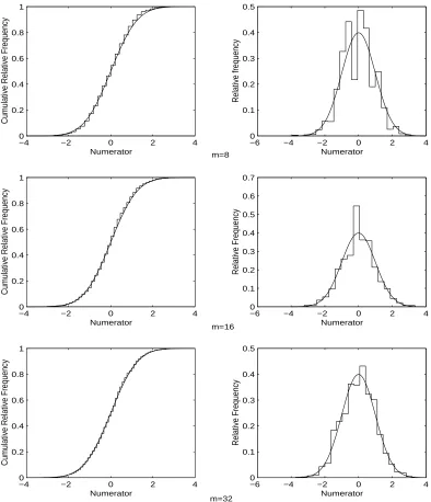
EAR(1) Process (3.78) with ϕ= 0.9 fork = 30 Batches of Size m. . . 76 3.43 Relative Frequency and Cumulative Relative Frequency of the

Numer-ator (3.31) of the t-Statistic (3.30) Based on 2000 Replications of the Alternating Correlation 2-State DTMC Defined by (3.65) and (3.66) for k= 30 Batches of Size m= 8, m= 16 and m= 32. . . 79 3.44 Relative Frequency and Cumulative Relative Frequency of the Squared

Denominator (3.32) of thet-Statistic (3.30) Based on 2000 Replications of the Alternating Correlation 2-State DTMC Defined by (3.65) and (3.66) fork = 30 Batches of Size m= 8, m = 16 and m= 32. . . 80 3.45 Relative Frequency and Cumulative Relative Frequency of the

Numer-ator (3.31) of the t-Statistic (3.30) Based on 2000 Replications of the High Positive Correlation 2-State DTMC Defined by (3.66) and (3.67) for k= 30 Batches of Size m= 16, m = 256 and m= 512. . . 81 3.46 Relative Frequency and Cumulative Relative Frequency of the Squared

Denominator (3.32) of thet-Statistic (3.30) Based on 2000 Replications of the High Positive Correlation 2-State DTMC Defined by (3.66) and (3.67) fork = 30 Batches of Size m= 16, m= 256 and m = 512. . . . 82 3.47 Relative Frequency and Cumulative Relative Frequency of the

Numer-ator (3.31) of the t-Statistic (3.30) Based on 2000 Replications of the Damped Sinusoidal Correlation 8-State DTMC Defined by (3.68) and (3.69) fork = 30 Batches of Size m= 16, m= 32 and m= 64. . . 83 3.48 Relative Frequency and Cumulative Relative Frequency of the Squared

Denominator (3.32) of thet-Statistic (3.30) Based on 2000 Replications of the Damped Sinusoidal Correlation 8-State DTMC Defined by (3.68) and (3.69) fork = 30 Batches of Size m= 16, m = 32 and m= 64. . 84 3.49 Relative Frequency and Cumulative Relative Frequency of the

Numer-ator (3.31) of the t-Statistic (3.30) Based on 2000 Replications of the M/M/1 Queue Waiting Times with Utilization τ = 0.9 for k = 30 Batches of Sizem = 16, m= 2048 and m= 4096. . . 85 3.50 Relative Frequency and Cumulative Relative Frequency of the Squared

Denominator (3.32) of thet-Statistic (3.30) Based on 2000 Replications of the M/M/1 Queue Waiting Times with Utilizationτ = 0.9 fork = 30 Batches of Sizem = 16, m= 2048 and m= 4096. . . 86 3.51 Relative Frequency and Cumulative Relative Frequency of the

(13)

3.52 Relative Frequency and Cumulative Relative Frequency of the Squared Denominator (3.32) of thet-Statistic (3.30) Based on 2000 Replications of the AR(1) Process (3.75) with ϕ = 0.9 for k = 30 Batches of Size m= 16, m= 32 and m= 64. . . 88 3.53 Relative Frequency and Cumulative Relative Frequency of the

Numer-ator (3.31) of the t-Statistic (3.30) Based on 2000 Replications of the EAR(1) Process (3.78) withϕ= 0.9 fork = 30 Batches of Sizem= 16, m= 32 and m = 64. . . 89 3.54 Relative Frequency and Cumulative Relative Frequency of the Squared

(14)

Chapter 1 Introduction

1.1 Problem of Confidence Interval Construction

in Steady-state Simulation

In discrete-event simulation, we are often interested in estimating the steady-state mean µX of a stochastic output process {Xi :i≥1} generated by a single, though

long, simulation run. Assuming the target process is stationary and given a time series of length n from this process, we see that a natural estimator of µX is the

sample mean, given by

X(n) = 1 n

n

X

i=1

Xi. (1.1)

We also require some indication of this estimator’s precision; and typically a confi-dence interval (CI) for µX is constructed at a certain confidence level 1−α, where

0< α <1.

If the Xi’s are independent and identically distributed (i.i.d.) random variables,

then the Central Limit Theorem (CLT) from classical statistics states that

√

nhX(n)−µX

i _D

−→

n→∞ N

0, σ_X2, (1.2)

where: σ2

X is the variance of the Xi’s, i.e., σ2X = E

h

(X1 −µX)

2i

, assuming this quantity is positive and finite; the symbol −→D

n→∞ denotes convergence in distribution;

and N(0, σ2

(15)

known, then an asymptotically valid 100(1−α)% CI for µX is

X(n)±z1−α/2

σX

√

n, (1.3)

where z1−α/2 is the (1−α/2)-quantile of aN(0,1) distribution. This means that

lim

n→∞Pr

(

µ ∈X(n)±z1−α/2

σX

√

n

)

= 1−α. (1.4)

If we construct a CI for µX on each of several prolonged runs of the simulation,

then the long-run proportion of these CIs which include (cover) the value µX is the

actual coverage probability. Normally, we would like the CI for µX to satisfy two

criteria: (a) the CI is narrow enough to be informative, and (b) the actual coverage probability of the CI is close to the nominal coverage probability 1−α. The CI (1.3) is based on a sample whose size n is fixed beforehand.

Another way of constructing a CI for µX is to continue sampling until some

pre-cision criterion is met. A prepre-cision requirement involving anabsolute half-length, δa,

specifies that the actual half-length of the CI given in (1.3) should be no larger than the threshold value δa, i.e.,

z1−α/2

σX

√

n ≤δa. (1.5)

A specification of arelative half-length, δr, implies that the CI half-length should be

no larger than the fractionδr of the magnitude of the final sample mean (e.g.,±10%)

so that

z1−α/2

σX

√

n ≤δr|X(n)|, (1.6)

assuming thatX(n)6= 0. If the process variance σ2

X is unknown, then a consistent estimator of σX2 can

be used in its place to construct a confidence interval for µX. Typically the sample

variance, given by

S_n2 = 1 n−1

n

X

i=1

Xi−X(n)

2

, (1.7)

is used to estimate σ2

X; and substituting Sn for σX in (1.3), (1.5), and (1.6) yields an

asymptotically valid 100(1−α)% confidence interval for µX as δa → 0 (Chow and

(16)

Unfortunately, observations of a simulation-generated output process are typically neither independent nor identically distributed. Therefore, the usual method of CI construction from classical statistics described above is not directly applicable. Sev-eral methods have been proposed for constructing CIs based on dependent observa-tions. Nonoverlapping batch means (NOBM) is one such method. Brief descriptions of other methods are given in Chapter 2.

1.2 Analysis of Steady-State Simulation Outputs

Using the Method of Nonoverlapping Batch

Means (NOBM)

In the NOBM method, the sequence of simulation-generated outputs {Xi : i =

1, . . . , n} is divided into k adjacent nonoverlapping batches, each of size mn. (In

later chapters we will wish to emphasize m’s dependence upon n; therefore we use the notation mn.) For simplicity, we assume that n is a multiple of mn so that

n = kmn; thus when k is fixed and mn → ∞, we have n → ∞. The sample mean,

Yj(mn), for the jth batch is calculated by

Yj(mn) =

1 mn

mXnj

i=mn(j−1)+1

Xi for j = 1, . . . , k. (1.8)

Then the grand mean Y(n, k) of the individual batch means, given by

Y(n, k) = 1 k

k

X

j=1

Yj(mn), (1.9)

is used as an estimator for µX (note that Y(n, k) = X(n)). Naturally, we seek to

construct a CI centered on the estimator (1.9).

(17)

output process could be readily determined from this information alone. Given that the simulation starts according to an initial distribution other than the steady-state distribution (e.g., the empty-and-idle state for a queueing system), some of the early observations of the selected output process will not be representative of the process in steady state. This is known as the initial transient orinitial bias problem, since a sample mean that includes these observations will likely be biased.

To overcome the initial transient problem, we start collecting statistics after an initial “warm-up” period. The number of observations that should be eliminated prior to the start of data collection is an area of research in itself. See, for example, Law and Kelton (1991) for a discussion. For purposes of this research, we plan to formulate a way to handle this initial bias problem in the context of the NOBM method for simulation output analysis. However, our primary focus will be on overcoming the problem of correlation between batch means and on the rate of convergence of the batch means to joint normality, since these issues affect the actual coverage of the confidence interval delivered by a batch-means procedure.

To continue the introductory discussion of NOBM methods for steady-state sim-ulation output analysis, we must introduce some basic nomenclature. For simplicity, we will assume the selected output process {Xj} is stationary (or stationary in the

strict sense), i.e., the joint distribution of theXj’s is insensitive to time shifts. If the

process{Xj :j = 1,2, . . .}is stationary, then for all positive integers r, p, j1, j2, . . . , jr

and for all real cutoff values x1, x2, . . . , xr, we have

Pr[Xj1 ≤x1;Xj2 ≤x2;· · ·;Xjr ≤xr] = Pr[Xp+j1 ≤x1;Xp+j2 ≤x2;· · ·;Xp+jr ≤xr].

A stochastic process{Xj}is said to beweakly stationary(or stationary in the wide

sense) if: (a) E[Xj] = µX for all j; and (b) the covariance between two observations

Xp and Xp+q, separated by q successive observations depends only on the lag q and

not on p,

γ(q)≡E [(Xp−µX) (Xp+q−µX)], q = 0,±1,±2, . . . . (1.10)

Stationary processes with a finite marginal variance are, therefore, weakly stationary. Processes that have a steady-state distribution are often weakly dependent, in the sense that Xj’s widely separated from each other in the sequence are almost

(18)

2) so that γ(q)→0 as q increases. These weakly dependent processes typically obey a CLT for dependent processes of the form

√

nhX(n)−µX

i _D

−→

n→∞ N

0, σ2, (1.11)

where

σ2 ≡ lim

n→∞nVar

h

X(n)i= ∞

X

i=−∞

γ(i) =γ(0) + 2 ∞

X

i=1

γ(i) (1.12) is the steady-state variance constant (SSVC) (as distinguished from the process vari-anceσ2

X). A sufficient condition for the SSVC to exist is that

P_∞

i=−∞|γ(i)|<∞; see,

for example, p. 459 Anderson (1971). Note that γ(0) = Var[Xi].

Although some output analysis methods attempt to estimate this steady-state variance constant σ2 _{for the construction of the CI (see Chapter 2), NOBM in its}

classical setting, i.e., when the number of batches is fixed, does not. NOBM seeks to make each batch a “repetition” of the experiment on the process. In order to achieve this, we assume that the batch size is sufficiently large so that the batch means {Yj(mn) : 1 ≤j ≤k} are i.i.d. normal,

{Yj(mn) : 1≤j ≤k}

i.i.d.

∼ NhµX, σ2(mn)/mn

i

, (1.13)

where the symbol ∼ is read “is distributed as,”

σ2(mn) = γ(0) + 2 mXn−1

q=1

1− q mn

γ(q), (1.14)

and Var[Yj(mn)] =σ2(mn)/mn. It follows that limmn→∞σ

2_(m

n) =σ2 and

Var[Yj(mn)]≈σ2/mn, (1.15)

provided that mn is sufficiently large.

We can now apply a classical result from statistics to compute a confidence interval for µX from the batch means {Yj(mn) : 1 ≤ j ≤ k}. If {Zj : 1≤j ≤k}

i.i.d.

∼

N(µZ, σZ2) so that the {Zi} constitute a random sample of size k from a normal

distribution with mean µZ and variance σZ2, then the sample mean Z(k) and the

sample varianceS2

k of the {Zj} are independent with

Z(k)∼N µZ,

σ_Z2 k

!

(19)

(k−1)S2

k

σ2

Z

∼χ2_k₋₁; (1.17)

and

Z(k)−µ

q

S2

k/k

∼tk−1, (1.18)

where tk−1 denotes the Student t-distribution with k − 1 degrees of freedom and

χ2_k₋₁ denotes the chi-square distribution withk−1 degrees of freedom. We can then construct an exact 100(1−α)% CI for µZ of the form

Z(k)±t1−α/2,k−1

Sk

√

k. (1.19)

Replacing Z(k) by X(n) and S2

k by the sample variance of the batch means

S_n,k2 = 1 k−1

k

X

j=1 h

Yj(mn)−X(n)

i2

(1.20) in (1.16)–(1.18), we have that (1.16)–(1.18) are approximately satisfied as the batch size mn becomes sufficiently large while the batch count k is fixed. This is because

the batch means Y1(mn), . . . , Yk(mn) become almost independent (since the process

is weakly dependent) and almost normally distributed (from an appropriate CLT for dependent processes). Brillinger (1973) showed the validity of the batch means method. Thus as mn → ∞ with k fixed so that n → ∞, an asymptotically valid

100(1−α)% confidence interval for µX is

X(n)±t1−α/2,k−1

S_√n,k

k. (1.21)

The asymptotic validity of NOBM depends on both the assumption of approximate independence of the batch means and the assumption of the batch means being ap-proximately normally distributed. The assumption that theYi(mn)’s are i.i.d. normal

random variables implies thatX(n) andS2

n,kshould be independent random variables.

If we are using a sampling technique that allows for varying the sample size, then our criterion for CI half-length can be specified using the t-statistic and the variance estimator S2

n,k. The requirement for an absolute half-lengthδa becomes

t1−α/2,k−1

S_√n,k

k ≤δa; (1.22)

and the requirement for a relative half-length expressed in terms ofδr has the form

t1−α/2,k−1

S_√n,k

(20)

Chapter 2 describes several procedures that have been proposed for implementing the NOBM method for CI estimation. These procedures address the problem of determining the batch size, mn, and the number of batches, k, that are required

to satisfy the assumptions of independence and normality. Theoretically, if these assumptions are satisfied, then we will get CIs whose actual coverage is close to the nominal coverage. However, because of the difficulty of the problem, research is still ongoing.

1.3 Scope and Objectives of Research

The primary objective of this research is to develop an easy-to-use, reliable batching method for constructing a CI for the expected response of a steady-state simula-tion model. This method, which we call Automated Simulasimula-tion Analysis Procedure (ASAP), has a theoretical basis, delivers specified accuracy and performs well on the basis of CI coverage in a variety of problems.

To provide a foundation for ASAP, first we investigate the asymptotic distri-butional properties of the vector of batch means along with the numerator and denominator of the NOBM t-ratio. Our research includes processes of the type

{f(Xn) :n≥1}, where {Xn : n ≥ 1} is a finite-state-space, Discrete-Time Markov

Chain (DTMC) andf(·) is a measurable function (e.g., a cost function associated with the occupied state). This is a nontrivial stochastic process for which a large body of literature exists. We also study other processes for which analytic expressions are available for the mean, variance, and correlations at all lags.

(21)

Some of the existing NOBM methods require intervention and interpretation by the user. Our method will remove the need for analysis and judgment calls by the user by specifying a beginning sample size, directing the user as to the amount of additional data necessary to achieve the requested precision, and ultimately delivering a CI.

The objectives of this research may be summarized as follows.

1. Investigate the convergence of batch means to joint normality and the conver-gence of the numerator and squared denominator of the NOBMt-ratio to their respective limiting distributions as the batch size increases with a fixed number of batches.

2. Develop theory and procedures, based on these convergence properties, for de-termining the batch size and the number of batches required for an asymptot-ically valid CI centered on the sample mean as the user-specified upper bound on the CI half-length tends to zero.

3. Formulate ASAP based on the foregoing analysis. ASAP operates as follows: the batch size is progressively increased with a fixed batch count until either

a) the batch means pass the von Neumann test for independence (Fishman 1978a), and then ASAP delivers the classical NOBM confidence interval (1.21); or

b) the batch means pass the Shapiro-Wilk test for multivariate normality (Tew and Wilson 1992), and then ASAP delivers a corrected confidence interval.

In case b), the correction is based on an inverted Cornish-Fisher expansion for the classical NOBM t-ratio (Hall 1983), where the terms of the expansion are estimated by fitting an autoregressive–moving average time series model to the batch means process.

4. Conduct an extensive experimental performance evaluation of ASAP, compar-ing it to other popular batch-means procedures in a broad range of stochastic systems.

(22)

1.4 Organization of the Dissertation

(23)

Chapter 2 Literature Review

In this chapter we will first discuss alternatives to NOBM in CI construction around the steady-state mean of a stationary weakly dependent process. A summary of the existing literature on NOBM will complete the literature review.

2.1 Methods of Confidence Interval Construction

2.1.1 Replication/Deletion

When employing the method of replication we simulatekindependent replicates, each of length n, of the process and obtain kn observations. Denote the ith observation within the jth replication (run) of the simulation model as Xj,i. Then

Xj(n) = n

X

i=1

Xj,i (2.1)

is the sample mean of the jth replicate, X(n) =

k

X

j=1

Xj(n) (2.2)

is an estimator of µX, and an asymptotically valid (1−α)100% CI is given by

X(n)±t1−α/2,k−1

Sk_√(n)

k , (2.3)

whereS_k2(n) = _k₋1₁Pkj=1

Xj(n)−X(n)

2

.Ifnis sufficiently large, (1.11) holds and Xj(n)∼· N

µx,σ

2

n

(24)

The method of replication causes the initial bias problem to be repeated k times, as opposed to the single long-run methods which encounter the problem only once. If the kindependent replicates are not started in steady-state and nis not large enough to dissipate the initial bias, then X(n) will be a biased estimator of µX. In this case

if we take k too large, then we run the risk of a narrow CI around a biased estimator of µX, which, therefore, may close in around the wrong value. Also n must be large

enough for the normality approximation of the replicate means to be in effect. In an effort to ameliorate the initial bias, Law and Kelton (1991), for example, make a case for deleting an initial portion of each replication before the sample aver-age is calculated and its CI is constructed; hence the name replication/deletion. Here again, we makekindependent replicates of lengthn, but we eliminate a predetermined number,`, of observations from each replicate. The time up to`is called the warm-up period. We include only the n−` observations in the calculation of the jth repli-cate sample mean, i.e., Xj(n, `) = _n1₋_`

Pn

i=`+1Xj,i. Now X(n, `) = 1_k

Pk

j=1Xj(n, `)

is a supposedly less biased estimator of µX and we have an asymptotically valid

100 (1−α) % CI generated by taking long enough replicates to achieve our desired coverage, i.e., as n→ ∞, PrhµX ∈X(n, `)±t1−α/2,k−1Sk√(n,`_k )

i

= 1−α.

Welch (1983) developed a graphical method for determining `. Law and Kelton (1991) propose using an n “much larger than the warm-up period ` determined by Welch’s graphical method.” How large n should be is an open problem; Law and Kelton (1991), for example, make no mention of how large n should be to meet the requirement of approximate normality of the replicate means.

Welch’s graphical method involves taking averages “across replicates” of the k occurrences of the ith observation, i.e., Xi = 1_k

Pk

j=1Xj,i. Moving averages, Xi(w),

at various windows w, of these Xi’s are plotted and ` is chosen to be greater than

the i where they seem to converge (Welch 1983).

The appeal of the replication/deletion method is its simplicity; it is easy to un-derstand and implement. It also has strong theoretical underpinning. From a compu-tational viewpoint, however, this method seems inefficient. We are “throwing away” ` observations from each replicate, a total of `k observations. In addition, to achieve k truly independent observations of Xj(n) we should make the determination of `

(25)

times.

2.1.2 Spectral Analysis

As mentioned in Chapter 1, some simulation output analysis methods, known as

consistent estimationmethods, seek to estimateσ2 _{(SSVC) and then use this estimate}

in constructing a CI for µX around the sample mean X(n). It is theoretically based

on the CLT for weakly dependent processes given in (1.11). Spectral analysis is one such method. We are assuming the discrete time stochastic process is stationary and is therefore weakly stationary.

We will assume that the series of covariances{γ(r) :−∞< r <∞}exists for the stationary discrete-time stochastic process we are simulating. The Fourier transform of this sequence is given by

f(λ) = 1 2π

∞

X

r=−∞

γ(r) cos (λr) ; (2.4)

where λ ∈ [−π, π] is called the frequency. The function f(λ) is the spectral density (see Anderson 1971). Obviously, from (1.12) it follows thatσ2 = 2πf(0), so we would like an estimate ˆf(0) of f(0), based on the nobservations X1, X2, . . . , Xn.

The natural estimator of the covariance γ(r) is

ˆ

γn(r) =

1 n

n_X−r

t=1

Xt−X(n) Xt+r−X(n)

. (2.5)

Given nobservations from the simulation, however, we can estimate at most (n−1) of theγ(r) terms in (2.4) with the corresponding ˆγn(r), so our estimator ofσ2 would

be

ˆ

σ_n2 = 2πfˆ(0) =

n_X−1

r=−(n−1)

ˆ

γn(r). (2.6)

Because of the large number of terms involved in the expression of the estimator ˆσ2

n,

this estimator’s variance does not go down to 0 as n → ∞. If we use a truncated

estimator _m

X

r=−m

ˆ

γ(r), (2.7)

(26)

To achieve a consistent estimator in the mean-square sense, i.e., MSEhfˆ(0)i → 0 as n → ∞, we require m → ∞ but m/n → 0. The MSE of the estimator ˆθ of a parameter θ is given by:

MSE(ˆθ) = Eθˆ−θ2

= Bias2(ˆθ) + Var(ˆθ). (2.8) See section 6.2.3 of Priestley (1981) for conditions under which this MSEhfˆ(0)i→0. Since we are assuming the process is weakly dependent, the sample covariances at the shorter lags tell us more about the dependency structure of the sequence than those at the longer lags. We can improve the estimator even further, if we could somehow weight these more informative ˆγn(r)’s, by using an estimator such as

2πfˆ(0) =

m

X

r=−m

wn(r) ˆγn(r), (2.9)

where wn(r) is an even function, called the lag window function, that is greatest

where r is close to 0 and decreases as r is farther from 0.

There are several weight functions that are frequently used in spectral density estimation. Two popular ones are Parzen and Tukey-Hanning (see, for example, Anderson 1971).

One weight function of particular interest is the modified Bartlett window func-tion, wn(r) = 1− |r|/m, which yields the following as the truncated sample spectral

density:

2πfˆ(0) =

(m_X−1)

r=−(m−1)

1− |r| m

!

ˆ

γn(r), (2.10)

form such thatm→ ∞ andn/m→ ∞asn→ ∞. It turns out that the overlapping batch means (OBM) variance estimator, defined below, is almost equal algebraically to the estimator of σ2 _{obtained through the spectral estimation method, using the}

modified Bartlett window as the weight function (see Section 2.1.3). Since we now have a consistent estimator ˆσ2

n for the SSVC σ2, we may now apply

the CLT in (1.11) to obtain the CI

X(n)±z1−α/2

ˆ σn

√

n. (2.11)

If the sample covariances are used to estimateσ2_{, it is computationally laborious.}

(27)

more efficient. Difficulties with the method lie in decisions that must be made on a weight function and on where to truncate (what value of m to use). The choice for m is the critical and complex issue (see Priestley 1981).

2.1.3 Overlapping Batch Means

The method of overlapping batch means (OBM), introduced by Meketon and Schmeiser (1984), divides thenobservations into batches of sizem, but each observation starts a new batch. The resulting number of batches is (n−m+ 1). The first batch contains observations X1, X2, . . . , Xm; the second batch, X2, X3, . . . , Xm+1, etc. Let

Xj(m) =

1 m

m_X−1

i=0

Xi+j (2.12)

denote the sample mean of the jth batch andX(n) the usual estimator ofµX.

Obvi-ously the Xj(m)’s are not independent, but are correlated. Meketon and Schmeiser

(1984) find that

d

VarhX(n)i= m n

n−_Xm+1

j=1

Xj(m)−X(n)

2

/(n−2m+ 1), (2.13)

the OBM estimator of VarhX(n)i, is approximately equal to 1

n−2m+ 1



_ˆγn(0) + 2 m_X−1

j=1

1− j m

ˆ γn(j)



 _(2.14)

which is approximately the estimator of 2πfˆ(0) derived via the spectral estimation method, using the modified Bartlett window. The approximate equality is the result of some end-effect terms in OBM (Damerdji 1991). So the OBM method of variance estimation is closely related to the spectral variance analysis (at frequency 0) method.

2.1.4 Regenerative Method

In order to apply the regenerative method of output analysis the process must be

regenerative, i.e., there exists an increasing sequence of random timesT1, T2, . . ., called

regeneration times, at which the process “starts over,” from a probability standpoint, independently of the past. The following hold: Pr [T1 <∞] = 1; Pr [0< τk<∞] = 1,

(28)

{Xs:s≥T1}; and the sequence{Xs :Tk ≤s < Tk+1}is an independent probabilistic

replica of the sequence {Xs :T1 ≤s < T2}.

The observations {Xi :Tk ≤i < Tk+1} form thekthregenerative cycle. If T1 ≥2,

then the process does not start in the regenerative state and is said to be delayed. An illustration of a regenerative process from queueing theory is the G/G/1 queue, where the regeneration times could be defined as the arrival times of customers who find an empty system.

LettingYj =P Tj+1−1

i=Tj Xi,{(Yj, τj) :j ≥1}is an i.i.d. sequence. If we continue with

our assumption that the process is stationary and also assume that it is regenerative, then we must haveτj is aperiodic. If EhPTi=2−T11|Xi|

i

<∞, then the steady-state mean of {Xi}is

µX =

E [Y1]

E [τ1]

. (2.15)

To apply this theory to the estimation of µX from simulation, we simulate, in

one long run, k regenerative cycles and obtaink observations of Yi and τi. The total

length of the run is denoted n(k) becausenwill depend on k. The sample estimator for µX computed from this method is

ˆ

µX(k) =

Y (k)

τ(k), (2.16)

where

Y (k) = 1 k

k

X

j=1

Yk =

1 n(k)

n_X(k)

i=1

Xi (2.17)

and

τ(k) = 1 k

k

X

i=1

τi. (2.18)

Although Y (k) and τ(k) are unbiased estimators of E(Yi) and E(τi), the quotient

Y (k)/τ (k) is not an unbiased estimator of µX.

The strong law of large numbers (SLLN) states that if V1, V2, . . . is a sequence

of i.i.d. random variables with E[Vi]=µV, E|Vi| < ∞ and if V(n) is the usual size n

sample estimator of µV,

lim

n→∞V(n) = µV, (2.19)

with probability (w.p.) 1. As a consequence of the SLLN, if E[PT2−1

i=T1 |Xi|]< ∞

and E[τ1]< ∞, then Y (k)/τ(k) is a strongly consistent estimator, i.e., as k → ∞,

(29)

Define a new random variable Zj =Yj −µXτj. Then E[Zj] = 0 and

σ_Z2 = Var [Zj] = E

h

(Yj−µXτj)

2i

= EhY_j2i−2µXE [Yjτj] +µ2XE

h

τ_j2i. (2.20) Because the Zj’s are i.i.d. random variables, under the condition that 0 < σ2Z <∞,

the CLT for the i.i.d. case holds, i.e., Z(k) q σ2 Z/k D −→

k→∞ N(0,1). (2.21)

Based on the k observations of Yj and τj, we can use the following to estimate σZ2:

ˆ

σ2_Z(k)≡ 1 k

k

X

j=1

Y_j2−2ˆµX(k)

1 k

k

X

j=1

Yjτj + ˆµ2X(k)

1 k

k

X

j=1

τ_j2. (2.22)

By replacing σ2

Z with ˆσZ2 (k) and dividing numerator and denominator by τ(k) in

(2.21) we obtain

ˆ

µX(k)−µx

r ˆ

σ2

Z(k)

k[τ(k)2]

D

−→

k→∞ N(0,1) (2.23)

Therefore, for k sufficiently large, an approximate asymptotically valid CI is:

ˆ

µX (k)±z1−α/2 q

ˆ σ2

Z(k)/k

τ(k) . (2.24)

The regenerative procedure described above is based on fixing the number of regenerative cycles k and simulating until that number of cycles has been observed. Shedler (1993) outlines a two-stage approach to implementing this procedure. A short preliminary pilot run is used to make estimates of µX, σ2Z and E[τ1] and then

the number k of required regenerative cycles for a relative length of ±100δr% is

determined by z1−α/2σˆZ

2

/(δµˆXτ(k))2, rounded up.

We can also use regenerative theory to obtain strongly consistent estimators and asymptotic CIs from a simulation of fixed length n. Now the observed number of regenerative cycles k depends onn; we will denote this dependency byk(n). Shedler (1993) points out (2.23) will hold whenkis replaced byk(n) and the resulting estima-torµx(k(n)) is strongly consistent with bias of order 1/n. Shedler (1993) also notes

(30)

The regenerative method is appealing for several reasons: it is easy to understand, eliminates the initial bias problem, and has truly i.i.d. observations. However, there are several disadvantages to this method. We must deal with identifying regenera-tion points, planning the simularegenera-tion length, and the possibility of a large amount of computation time. The cycle lengths are unknown prior to the actual running of the simulation and may be very long. Therefore, an extremely long simulation may be required to observe only a few cycles. Because the estimators are ratios, Bratley, Fox, and Schrage (1987) are suspicious of CIs, based on (asymptotic) normality, applied to finite sample sizes.

2.1.5 Autoregressive Method

The Autoregressive Method introduced in the simulation context by Fishman (1973, 1977, and 1978b) assumes a covariance stationary process, which is implied by our assumption of strict stationarity. The other assumption required for this method is that the process is well represented by the autoregressive model:

p

X

j=0

bj(Xi−j −µX) =i, fori=p+ 1, p+ 2, . . . (2.25)

where p is the order of the model, b0 = 1, µX =E[Xi], and {i} is assumed to be an

i.i.d. sequence of random variables with E[i] = 0 and Var[i] =σ2 (Law and Kelton

1991).

It can be shown that if the process {Xi : i = p, p+ 1, . . .} satisfies (2.25), then

nVar[X(n)] → σ2/Pp_j₌₀bj

2

as n → ∞. Fishman’s procedure (Fishman 1973) allows for making sample estimators of the order ˆp; the constants ˆbj forj = 1, . . . ,p;ˆ

and the variance ˆσ form the sample estimators of the covariances ˆγ(q). If ˆb =

1 +Pˆpj=1ˆbj, then

d

VarhX(n)i= σˆ

2

n2_(b) (2.26)

is the sample estimator of Var[X(n)]. The 100(1−α)% CI for µX is :

X(n)±t_{f ,}ˆ₁₋_α/₂ r

d

VarhX(n)i, (2.27)

where ˆf is the estimated degrees of freedom given by: ˆ

f = nˆb

2Pˆp_j₌₀(ˆp−2j) ˆbj

(31)

Although Wold’s Decomposition Theorem (Anderson 1971) tells us that any sta-tionary sequence can be written as an infinite order autoregressive model, in the application to simulation output analysis we must of course restrict our model to finite order and to parameters which are sample estimates. In the end, we run the risk of not adequately describing the process.

2.1.6 Standardized Time Series

The method of Standardized Time Series (STS), introduced by Schruben (1983), is a so-called “cancellation” method because in a certain limit theorem the SSVC, σ2, cancels out and there is, then, no need to estimate it. The STS method assumes that a functional central limit theorem (FCLT) for the (standardized) partial sums of the process is in force. Such a result holds for processes that are weakly dependent in the sense we discussed earlier, i.e., observations that are far from each other in time are almost independent. See the end of this section for a discussion of processes which obey a FCLT.

If X1, . . . , Xn are observations obtained from the simulation of the process and

E[Xi] = µX, then we know from (1.11) that

√

nX(n)−µX

_D

−→

n→∞ σN(0,1). Let

the partial sum process be given by Sn=

n

X

i=1

Xi, n= 1,2, . . . . (2.29)

Then from the SLLN, under regularity conditions, Sn/n → µX w.p. 1 as n → ∞,

and from the CLT, √n(Sn/n−µX) D

−→

n→∞ σN(0,1). Now let

Yn(t) =

S[nt]

n , 0 ≤t≤1, (2.30)

where [nt] is the integer portion of nt. Schruben (1983) explains that the range of t is [0,1] as a part of “standardizing” the series, by transforming its length to unit length. Again, from the SLLN, we can show thatYn(t)→µXt with probability 1 as

n→ ∞.

Now consider the function Zn(t) =

√

n S[nt]

n −µXt

!

(32)

Note thatZn(t) is a function int, but for given t, Zn(t) D

−→

n→∞ N(0, σ

2_{t) by the CLT.}

We are now ready to state the FCLT for weakly dependent processes: Zn(·)

D

−→

n→∞ σB(·), (2.32)

where {B(t) : t ≥ 0} is the standard Brownian motion process. Brownian motion is characterized by the following properties:

• B(0) = 0;

• {B(t) :t≥0} has continuous sample paths;

• {B(t) :t≥0} has stationary and independent increments;

• for every t >0, B(t) is normally distributed with mean 0 and variancet. For t= 1, (2.32) may be written

Zn(1) =

√

n

_S

n

n −µX

D

−→

n→∞ σB(1) D

=σN(0,1), (2.33)

where = means equality in distribution.D

To employ (2.33) in constructing a CI, we would have to know σ. However, a function g of {Sn : n ≥ 0} can be chosen to cancel the scaling constant σ. The

continuous function g :C[0,1]→ <, should have the following properties (Glynn and Iglehart 1990):

• g(αx) =αg(x), forα >0 and for all x∈C[0,1],

• g(x−βk) =g(x) for all β∈ < and x∈C[0,1], where k(t) =t,

• Pr[g(B)>0] = 1,

• Pr[B ∈D(g)] = 0.

(33)

By application of the continuous mapping theorem and the converging-together theorem, (see Glynn and Iglehart 1990, for details) we have that if g is a function with the above properties, then

Zn(1)

g(Zn) D

−→

n→∞

σB(1) g(σB) =

σB(1) σg(B) =

B(1)

g(B) . (2.34)

The SSVC σ2 _{does not appear in the right-hand side limit, and, therefore, need not}

be estimated. To apply the STS method, we must find a functiong to use, as well as the distribution of B(1)/g(B).

Glynn and Iglehart (1990) show that NOBM, where the number of batches is fixed, is a STS method. They define the functiong by:

gk(x) =

"

k k−1

! _k

X

i=1

(∆kx(i/k)−x(1)/k)2

#1/2

, (2.35)

where ∆hx(t) =x(t)−x(t−1/h). It can be shown thatgk has the properties listed

above (see Glynn and Iglehart 1990 for details). Now ∆kB(i/k) for i = 1, . . . , k

are increments of standard Brownian motion, i.e. are i.i.d. normal random variables with zero mean and variance 1/k. The quantity B(1)/k is the sample mean of these increments and therefore,B(1)/gk(B) has a Student’st-distribution withk−1 degrees

of freedom. The functiong(Zn) is equal to

√

nSn,k/

√

k, whereSn,kis given in (1.20).

Glynn and Iglehart (1990) give the functions that correspond to the STS area and maximum methods, introduced by Schruben (1983).

We now discuss some processes which obey a FCLT and therefore are candidates for application of the STS method. Glynn and Iglehart (1990) list the following as processes for which the FCLT exists: stationary (and some non-stationary) φ-mixing processes, strictly stationary strongly mixing processes, associated strictly stationary processes, and regenerative processes. Let Fv

u be the σ-field of events generated by

the processXu, Xu+1, . . . , Xu+v. Mathematically, the process{Xi}is strongly mixing

if, for all k ≥1,

sup

Q∈Fk

1,F∈Fk∞+j

|Pr (Q∩F)−Pr (Q) Pr (F)| ≤αj, (2.36)

where limj→∞αj = 0, and φ-mixing if

sup

(34)

where limj→∞φj = 0.

Although φ-mixing is stronger than strongly mixing, both of these definitions imply that events far from each other in time are almost independent. We have previously discussed, in Section (2.1.4), what it means for a process to be regenerative. Schruben (1983) states that m-dependent processes also qualify as φ-mixing if m is bounded. Using the notation above, a process is m-dependent if the σ-fieldsFk

1 and F∞

k+m+1 are independent (for all k≥1).

2.2 Fixed Sample Size Approaches to NOBM

2.2.1 Classical NOBM

We use the termclassicalNOBM to refer to the nonoverlapping batch means method when the number of batches is held fixed. If we fix our sample sizenandthe number of batches k prior to running the simulation, then we have to live with whatever CI results (it may be too wide to be informative). We would like to choosek andm that give us the “best” results. Let

Hα,k(n) =tα/2,k−1

S_√n,k

k (2.38)

denote the half-length of the CI given in (1.21). Although here we are considering n to be fixed, other procedures using NOBM allow nto change. Schmeiser (1982) gives the assumptions of the method of NOBM as:

1. Initial transient effects have been removed;

2. For a run length of n, a number of batches k∗ and associated batch size m∗ = n/k∗ exist such that the dependency and nonnormality of the batch means are negligible for m≥m∗ and k≤k∗; and

3. The problem of n/k not being integer is insignificant.

Note that assumption 2 above implies that n is large enough so that dependency and nonnormality is negligible for some k.

(35)

would like Prh|X(n)−µX| ≤Hα,k(n)

i

'1−α. Based on this criterion alone, k = 2 is the best choice because it yields a largeHα,k(n), which in turn means that our CI

will have a high probability of covering the mean. However, Hα,k(n) may be so large

that we do not achieve an informative CI. Also, Pr[|X(n)−µX| ≤Hα,k(n)] will most

likely be larger than 1−α in actuality.

We might wish to consider the second criterion, E[Hα,k(n)]. These two

crite-ria compete with each other so there is a trade-off between expected half-length and coverage. Other measures Schmeiser (1982) considers are: the standard devia-tion of the half-length, qVar[Hα,k(n)], the coefficient of variation of the half-length,

CV[Hα,k(n)]≡

q

Var[Hα,k(n)]/E[Hα,k(n)], and for all µ1 6=µX, the function

βα,k(µ1)≡Pr h

|X(n)−µ1| ≤Hα,k(n)

i

. (2.39)

This function may be thought of as the probability of a type II error in hypothesis testing. Therefore, smaller βα,k(µ1) for µ1 6=µX means better performance.

Based on properties of the half-length, Schmeiser’s (1982) results, derived ana-lytically indicate that more batches are needed for smaller α (i.e., higher confidence levels). However, a number of batches larger than 30 had negligible effect on the properties of the half-length.

Schmeiser (1982) favors the function βα,k(µ1) as a performance measure, since it

takes into account both X(n) and Sn,k together, as opposed to the moments of the

half-lengthHα,k(n) which are functions ofSn,k only. Also,βα,k is a coverage function,

directly related to coverage of the mean, which was our first criterion for an acceptable k.

Plots of the coverage function βα,k(µ1) (Schmeiser 1982) in terms of covering

points removed from the actual mean µX by factors δk of the Var[X(n)] show that

the decrease in βα,k(µ1) due to increasing k by 1: (a) decreases as k increases, (b)

decreases as α increases, and (c) is small when δk<1.

(36)

2.2.2 Nonclassical NOBM

One approach to fixed sample size NOBM starts with a fixed total sample size of n and allows for varying the number of batches k and consequently the batch size m. Fishman (1978a) proposed a procedure for determining batch size for a sample of size nwhich relies on a statistical test for independence between batch means. Letρ1(m)

denote the lag-one correlation:

ρ1(m)≡Corr [Yj(m), Yj+1(m)]. (2.40)

The von Neumann test for independence tests the null hypothesis H0 : ρ1(m) = 0

using the statistic:

Ck= 1−

Pk−1

j=1(Yj(m)−Yj+1(m))2

2Pk_j₌₁Yj(m)−X(n)

2 . (2.41)

If the Yj(m)’s are normally distributed, then under H0,

Ck ∼· N 0,

k−2 k2−₁

!

, (2.42)

for k as small as 8. Fishman (1978a) points out that for small m it is doubtful that the Yj(m)’s are normally distributed. However, if n is large then k is large

(when m is small) and the large sample properties suggest that we can approximate the distribution ofCk/

q

(k−2)/(k2−_{1) with the}_N_(0,_{1) distribution, provided that}

the Yi(m)’s are independent and identically distributed. Also as m increases (and

k decreases) we expect that the distribution of the Yi(m)’s approaches the normal

distribution and we can reasonably assume approximate normality of theCkas long as

k ≥8. If the covariance is assumed to be a monotone decreasing function, then a one-tail test is appropriate. So if we desire a level β test (level β means the Pr [ rejecting H0|H0 is true ] ≤ β), then we will accept the null hypothesis that ρ1(m) = 0 if

Ck≤z1−β

q

(k−2)/(k2−_1).

Fishman’s (1978a) algorithm (given in Figure 2.1 begins with a total sample size of n. On the first iteration, the batch size, m, is set to one; the number of batches, k, is set to n; and the batch means Y1(m), . . . , Yk(m) and the test statistic Ck are

(37)

1. m←1. 2. k ← bn/mc.

3. Ifk < 8, then return indicating failure.

4. Compute the batch meansY1(m), . . . , Yk(m) using (1.8).

5. Compute Ck using (2.41).

6. IfCk> z1−β

q

(k−2)/(k2−_1),_{then take} _m←_2m _{and go to 2.}

7. Otherwise, m∗ ←m and k∗ ←k. 8. Compute S2

n,k∗ using (1.20).

9. Return with (1−α)% CI constructed using (1.21).

Figure 2.1: Fishman’s Fixed Sample Size Algorithm for Determining Batch Size m and Number of Batches k.

the form (1.21) is constructed. If the batch size becomes so large that the number of batches k <8, then the algorithm fails to determine an optimal batch size k∗.

Fishman(1978a) tested the algorithm with the M/M/1 queue, varying both the utilization factor and the run length. Sixty replications at each level of utilization and each value ofnwere made. If the algorithm failed to determinem∗, the algorithm was terminated. In general, larger initial ngave better coverage, although most fell short of the nominal 95%. The poorest performance was on the cases where utilization was high, but the sample size was small. Relatively few replications failed to find an m∗ and those which did fail were at the higher levels of utilization and lower values of starting n.

Fishman (1978a) shows that underestimation of the variance becomes worse for fixed n and increasing utilization. He suggests that a potential source of error in the algorithm is underestimation of them∗ required for independence of the batch means, thereby resulting in an estimated variance which is too small. This prompted him to increase β and thereby impose a stronger requirement for independence. The higher β is, the more likely we are to reject H0 whether it is true or false. So by increasing β

we will increase the Pr [ rejecting H0|H0 is false ] which would seem to be our primary

(38)

in using at distribution is generally regarded as being insensitive to this departure.” Fishman theorizes that a short sample where the observations are highly correlated (as in the M/M/1 queue with utilization 0.9) may be insufficient to disclose the variation in the underlying stochastic process and we can only improve performance by increasing n.

Song and Schmeiser (1995) investigate the effects of batch size m on the mean square error (MSE) of the variance estimator. They seek the optimal batch size which yields the minimum MSE. However, we do not know how the coverage of the CI is affected by choosing a batch size based on this criterion. The MSE of the variance estimator is given by:

MSEVardhX(n)i= EVardhX(n)i−VarhX(n)i2

= Bias2VardhX(n)i+ VarhVard hX(n)ii, (2.43) where Bias ≡EhVardhX(n)i−VarhX(n)ii. Song and Schmeiser (1995) derive an approximation of the MSE of the variance estimator as a function of m:

MSEVar (m)d ≈ c

2

bγ12

n2_m2 +

mcvγ20

n3 !

γ2(0). (2.44) The optimal batch size is given by:

m∗ ≈



2n c

2

b

cv

!

γ1

γ0

!2

 1/3

, (2.45)

where cb and cv depend on the method of variance estimation being used. The ratio

γ1/γ2 is called the balance point, where γ1 ≡

P_∞

h=−∞ρh = 1 + 2

P_∞

h=1ρh and γ0 ≡

P_∞

h=−∞|h|ρh = 2

P_∞

h=1hρh and ρh is the correlation at lag h, for the underlying

process Xi :i= 1,2, . . ..

The sensitivity of the MSE at points close tom∗ was also considered by calculating the second derivative of (2.44). Song and Schmeiser (1995) considered four variance estimation methods. Using our notation, the estimator they study for NOBM is (1/k)S2

n,k. For NOBM they givecb = 1 andcv = 2. While NOBM compares favorably

(39)

Based on their asymptotic results, Song and Schmeiser (1995) give the following as the approximate optimal MSE batch size for a finite sample of size n:

~

m∗ ≈1 +



_2n c2b

cv

!

γ1

γ0

!2

 1/3

, (2.46)

where γ0 and γ1 are estimated from the data. Song and Schmeiser (1995) give

em-pirical results for the OBM method.

2.3 Sequential Approaches to Batch Means

In using the fixed sample size procedure, we have assumed that the fixed total sam-ple size is large enough that dependence and nonnormality of the batch means is negligible. We are then forced to live with whatever length of CI results. Often the resulting CI is too wide to be informative, i.e., it does not possess the desired length. Sequential procedures, however, allow for increasing the sample size at each iteration. In this work, we are concentrating on the NOBM method of CI construction and will therefore discuss in some detail sequential procedures which have been proposed for the NOBM method. However, it should be mentioned that sequential procedures exist for other methods, for example Lavenberg and Sauer (1977) and Fishman (1977) discuss sequential procedures for regenerative simulations and Heidelberger and Welch (1981a, 1981b, and 1983) use sequential procedures in a spectral estimation context.

2.3.1 Law and Carson’s Procedure

Law and Carson (1979) developed a sequential procedure for NOBM for covariance stationary processes. They point out three potential sources of error when the method of NOBM is used: (i) bias in the estimator ˆσ2 _{due to a batch size}_m _{that is too small}

for the Yj(m)’s to be uncorrelated, (ii) nonnormality of the Yj(m)’s, and (iii) the

process {Xi} may not in fact be covariance stationary. Law and Carson discount the

effect of nonnormality for a number of batches k ≥ 20 and focus on the problem of bias caused by correlation of the batch means.

The fixed number of batches (FNB) rule calls for fixing the number of batches and sequentially increasing the batch size until the sample lag-one correlation estimator of ρ1(m) between batch means is less than some specified level, e.g., ˆρ1(m) ≤ 0.05.

(40)

However, empirical studies have shown we may quite often achieve an acceptable ˆ

ρ1(m) when in fact it can be shown analytically thatρ1(m) is greater than the specified

level. The problem is that estimators of correlation are biased and have large variance when the number of samples is small. Law and Carson (1979) found that some systems required as many as 400 batches for a precise estimate of ρ1(m).

This prompted them to investigate the possibility of using `kbatches of size mto make inferences about the correlation between k batches of size`m. Law and Carson (1979) chose 34 stochastic processes whereρ1(m) could be computed analytically and

plotted ρ1(m) vs. m. Three types of behavior were observed: (i) lag one correlation

strictly decreases to zero, (ii) lag one correlation changes directions (one or more times) then strictly decreases to zero, and (iii) lag one correlation is less than zero.

The algorithm (given in Figure 2.2 from Law and Carson (1979) begins by fixing a level of correlation,c, as a stopping value; a relative half-length,γ >0; and positive integers `, k, n0, n1 (`k even, `k/2 even, n0 < n1 < 2n0 each divisible by `k). Then

n1 observations are collected. The observations are divided into `k batches of size

m. The lag one correlation coefficient is calculated from these observations using the jackknifed estimator:

ρ₁(`k, m) = 2ˆρ1(`k, m)− h

ˆ

ρ1₁(`k/2, m) + ˆρ2₁(lk/2, m)i/2, (2.47) where ˆρ1₁(`k/2, m) and ˆρ2₁(`k/2, m) are the usual lag one correlation estimators based on the first and last lk/2 batches, respectively. Law and Carson use this jackknifed estimator because in general it is less biased.

(41)

0. Fix positive integers `, k, n0, n1(`k even, `k/2 even, n0 < n1 <2n0, n1

and 2n0 each divisible by `k), the stopping value c > 0, the relative

half-lengthγ >0; let i= 1; collect n1 observations.

1. a. Divide theniobservations into`kbatches of sizem=ni/(`k).Compute

ρ₁(`k, m) from Yj(m) (j = 1, . . . , `k). If ρ1(`k, m) ≥ c, GO TO 2. If

ρ₁(`k, m)≤0, GO TO 1c. Otherwise, GO TO 1b.

b. Divide ni into `k/2 batches of size 2m. Compute ρ1(`k/2,2m) from

Y1(2m), . . . , Y`k/2(2m). If ρ1(`k/2,2m) < ρ1(`k, m), go to 1c.

Other-wise, GO TO 2.

c. Divideniintokbatches of size`m. ComputeX(ni) andSn2i,k. Compute

the half-length Hα,k(ni) using (2.38). If |Hα,k(ni)/X(n)| < γ, then

construct a confidence interval using (1.21) and STOP. Otherwise, GO TO 2.

2. i ← i+ 1. ni ← 2ni−2. Collect the additional ni −ni−1 observations

and GO TO 1a.

Figure 2.2: Law and Carson’s Sequential Algorithm for Determining Batch Size m and Number of Batches k.

lk batches of size m; when, in the end, k batches of size lmare used for the variance estimator. (See Law and Carson 1979 for details on the relationship ofρ(m) toρ(lm).)

2.3.2 Fixed Number of Batches (FNB)

If the process{Xi :i= 1,2, . . .}is weakly stationary for batch sizem, then the batch

means process {Yj(m) : j = 1,2, . . .} is also weakly stationary. If mn ≡ n/k, it can

be shown that (Alexopoulos and Seila 1996, for example): Var[X(n)] = Var[X(mn)]

k 1 +

nVar[X(n)]−mnVar[X(mn)]

mnVar[X(mn)]

!

. (2.48)

If we fix k and let n → ∞ then Var[X(n)]/Var[X(mn)]/k

→1. This leads to the FNB rule: fix the number of batches and let the batch size mn increase as the total

sample size n increases. The FNB rule has some limitations. (See Alexopoulos and Seila 1996 and Fishman 1996.) The sample estimator mnSn,k2 , when k is fixed, is not

(42)

than ones constructed using a consistent estimator. Also, statistical fluctuations in the half-length of the CI do not diminish relative to statistical fluctuations in the sample mean. Fishman (1996) characterizes this behavior as “unappealing,” particularly compared to the i.i.d case, but does not comment on its relative significance.

2.3.3 Square Root Rule (SQRT)

The problems with the FNB rule lead us to consider a scheme where both the number of batches kn and the batch size mn grow as the total sample size n does. Here the

number of batches is indexed by n to indicate that it is a function of the sample size. The SQRT rule is such a procedure where, kn and mn are chosen such that

limn→∞n1/2mn = 1 and limn→∞n1/2kn = 1. This method, however, tends to

un-derestimate Var[X(n)] for fixed n, which results in poorer coverage. See Fishman (1996).

2.3.4 LBATCH and ABATCH Procedures

We see that both the FNB and SQRT rules have advantages and disadvantages. Although for a given nthe FNB rule yields CIs with better coverage than the SQRT rule (because of SQRT rule’s tendency to underestimateσ2_{), the mean CI length tends}

to exceed that of the CI generated from the SQRT rule. For both rules, however, the coverages of the generated CIs approach 1−α asn→ ∞. So the SQRT rule exhibits greater statistical efficiency asn→ ∞. See Fishman (1996) for graphical comparisons of the behavior of the variance estimators and coverage properties of the FNB and SQRT rules.