Implicit filtering for constrained optimization and applications to problems in the natural gas pipeline industry

(1)

Implicit Filtering for Constrained Optimization and

Applications to Problems in the Natural Gas Pipeline

Industry

1 Alton Patrick

Department of Mathematics

Center for Research in Scientific Computation

North Carolina State University

Advisor: Tim Kelley

April 26, 2000

(2)

Chapter 1 Introduction to Optimization

The goal of an optimization problem is to find a point in the domain of the objective function

such that is “optimal.” “Optimal” can mean either a minimum or maximum of . However,

a maximum of is a minimum of , so we can express every optimization problem as a search

for a minimum of some . Therefore, the optimal point

is given by

(1.1)

where is the set of points near and is the objective function. If is bounded in some

way, we call (1.1) a constrained optimization problem. If is , (1.1) is an unconstrained

optimization problem.

1.1 Basic Solution Strategy

Let’s consider a very simple optimization problem, with! . We will call our first guess at

a solution!" . Subsequent (hopefully educated!) guesses at the solution will define a sequence of

iterates, #$!%'&)( *,+.- .

Clearly has a minimum at /- . The solution to a serious optimization will rarely be so

obvious. The initial iterate!" is usually a genuine guess, perhaps based upon a graph of showing

the approximate position of the solution, perhaps based upon nothing at all. Let’s pretend we are

ignorant about the location of the minimum and choose!"021 .

Now we need a way to get from !" to 43 . We would like to move towards the minimum, so

it would be good if 435768!" . The derivative of at !" , 9!": , tells us which way to go

from!" to reduce the objective function. If 9 !": is negative, moving to the right will reduce the

function value. If 9!": is positive, moving to the left will reduce the function value. In general,

moving along the x-axis in the direction of 9!": will reduce the objective function. 9!": is

therefore called a descent direction.

How far should we move in this descent direction? The simplest thing would be to set

43;!"<=

9

!" >1?@1?AB1CD?1

This is unproductive, because !":ED43F and we are no better off than when we started. The

solution is to multiply9!": by a factorGIHJK-L(MON.G is called the step length. Then43 is given by

43;!"<=G

9

!":

(4)

4 CHAPTER 1. INTRODUCTION TO OPTIMIZATION

We can try different values ofP , starting withP,QSR , until we find anT4U that produces an acceptable

value ofVWT4UFX . This process is called a linesearch.

Two questions immediately arise:

1. “What sequence of values should be used forP ?” and

2. “What is an ‘acceptable’ value forVWT4UFX ?”

Often, the first question is answered by taking

PZY=Q[ Y]\_^ Q` \ R \ ab\ccdc (1.2)

where`feg[he2R . More sophisticated ways to choose a sequence ofP ’s will be discussed later.

Answering the second question requires that we define the concept of sufficient decrease. This

means establishing a criteria to check that VWT4U5X is ”sufficiently” smaller than VWT!i:X . One such

criteria isVWT4UFXje.VWT!i X . This is called simple decrease. Using the simple decrease condition, we

would take as the step length the firstPZk such that

VWT!iml@PZknVoWT!i X5X0epVWT!i:X

Unfortunately, simple decrease is usually too simple. It can lead to taking very small steps that cause the iteration to stagnate at one point. We will use a more complicated idea of sufficient decrease called the Armijo rule. This requires that

VWT!i<l@PVoWT!i:XFXl=VWT!i X0e2lrqPstVoWT!i:X$su

where`fevqJeR . TypicallyqwQSR$`)x)y .

So far we have looked at a problem only in one dimension, to make the basic solution plan

easier to follow. We want to be able to solve problems where T{z}|~ . Generalizing what we

have done so far to n dimensions is fairly straightforward. The N-dimensional equivalent of the derivative is the gradient,

VQ V T4U \ V T u \cdccd\ V TC c l

V gives a descent direction forV in N dimensions just asV

o does in one dimension. The Armijo

rule for sufficient decrease in N dimensions is

VWT!l=P VWT!XFXl=VWT!Xje>lrqP VWT!X' u c (1.3)

Using the gradient, we can generalize the above method for use in N dimensions. We will also

introduce the notationT! to represent the current point in the iteration andT to represent the next

(5)

1.2. TERMINATION CRITERIA 5

Algorithm 1 Steepest Descent Pick! .

Set!.!

while! is not the minimum of do

Find such that (1.3) is satisfied.

Setp!=7!

Set!; .

end while

1.2 Termination Criteria

One issue Algorithm 1 dodges is how to know when ! is the minimum of . Two theorems

will give us necessary and sufficient conditions to know that! is an optimal point. For proofs of

these theorems, see [6].

Before giving those theorems, we must define some more terms. We let represent the

Hessian of , where

tE

¡

We also define the terms positive semi-definite, positive definite, and symmetric positive definite (spd).

Definition 1 A matrix A is positive semi-definite if Z¢£].¤¦¥L§¨.©.ª¬« . £ is positive definite

if Z¢£rS®¥L§¨{©{ª¬«¯§F±°²¥ . If £ has both positive and negative eigenvalues, we say £ is

indefinite. IF£ is symmetric and positive definite we say£ is spd.

Now we can present the two theorems which give the termination criteria for Algorithm 1.

Theorem 1 Let³ be a local minimizer of . Thenf:³_ is positive semidefinite and

7

³

2¥

¡

Theorem 2 Assume that ³ ´µ¥ and that ¶³ is positive definite. Then ³ is a local

minimizer of .

From these two theorems, it is clear that we would like to stop when !r/¥ . However,

it is very unlikely that we will be lucky enough to land exactly on the minimum. Even if we do,

it might take a very large number of iterations, many of which would only move! a very small

distance. So we will simply stop when7! is “close” to zero. We can use ·O!$· , the norm

of! , to measure how close to zero7! is. One way to check that the gradient is “close”

to zero is to see if ·O7!'· is significantly smaller than ·O7!:'· , i.e.

·O!$·?¸º¹:»¼·O!:$·

where ¥º¸¦¹:»I¸²½ . However, if ·O7!:'· is very small, it may not be possible to satisfy this

condition with floating point numbers. So we add an absolute tolerance,¥¸=¹d¾¿¸½ :

·O!$·?¸=¹O»À·O!¶'·Á@¹O¾

¡

(6)

6 CHAPTER 1. INTRODUCTION TO OPTIMIZATION

This algorithm might fail to find a minimum or take a very long time to find a minimum. Therefore, it is useful to limt the number of iterations the algorithm will go through. From now on,

our algorithms will incorporate a limit,ÂbÃ¬ÄÀÅ , on the number of iterations.

1.3 Refining the Descent Direction

We have been using ÆÇ7ÈÉÅ!ÊË as the descent direction. The linesearch method becomes more

general if we replaceÆÇ7ÈÉÅ!ÊË with a general descent direction,Ì . With this change, the sufficient

decrease condition, 1.3, becomes

ÈÉÅ!Ê4ÍºÎÌ ËÆ=ÈÉÅ!ÊËjÏpÐÎÇ7ÈÉÅ!ÊËÒÑÌ!Ó (1.5)

We will consider descent directions based on quadratic models of È . Just as quadratic models

of functions inÔIÕ require information about the second derivative, quadratic models of functions

intÔ¬Ö require information about the Hessian. We will use models of the form

Ã×ÉÅËØ>ÈÉÅ!ÊÙËÚÍgÇ7ÈÉÅ!ÊËÙÑÉÅÆhÅ!Ê5ËÚÍÜÛÝ ÉÅ7ÆhÅ!Ê5ËÙÑÞ´Ê ÉÅÆhÅ!ÊË (1.6)

where Þ´Ê is an approximation to the Hessian of È called the model Hessian. Þ´Ê is used instead

of the actual Hessian because 1.) the Hessian of È may not be known or may be too costly to

calculate; and 2.) Þ´Ê is required to be spd, a requirement that the actual Hessian may not meet.

The reason for this requirement is discussed later.

Minimizing Ã is, in general, easier than minimizing È because we have a simple expression

forÃ . Setting the gradient ofÃ equal to zero gives

ÇÃ×ÉÅß5ËØÇ7ÈÉÅ!ÊËÚÍºÞ´Ê:ÉÅßàÆhÅ!ÊËØ2á (1.7)

whereÅ

ß is the minimum of

È . Note thatÅ

ß is only a minimum of

È ifÞfÊ is positive definite (see

Theorem 2). We want to move fromÅ!Ê toÅ

ß because the minimum of

È is likely to be close to the

minimum ofÃ . So we setÌâØãÉÅ

ß

ÆäÅ!ÊË, or, using (1.7) ÌâØSÆÞ×å

Õ

Ê

Ç7ÈÉÅ!ÊË (1.8)

(1.8) may not give a descent direction if Þ´Ê is not spd [6]. To insureÞ´Ê is spd, we usually let

Þ´æ be a clearly spd matrix (such as the identity) and then use one of two methods which guarantee

symmetric positive definiteness to updateÞ´Ê as the iteration progresses. If we letç?ØpÅèÆÅ!Ê and

é

ØÇ7ÈÉÅèêËÆ@Ç7ÈÉÅ!ÊË , then the first update formula, called BFGS update, is ÞfèëØ2Þ´ÊÍ é é Ñ é Ñ ç Æ ÉnÞfÊç'ËOÉKÞ´Êç'Ë Ñ ç Ñ Þ´Êç Ó (1.9)

The second update formula, SR1, is

ÞfèIØ;Þ´Ê4Í É é Æ@Þ´Êç'ËOÉ é ÆJÞ´Êç'Ë Ñ É é Æ@Þ´Êç'Ë Ñ ç Ó (1.10)

Both of these techniques can be adapted to update the inverse Hessian instead of the Hessian itself.

This is more useful since we only need Þ

å

Õ

Ê , not

Þ´Ê , to findÌ . Optimization methods that update

(7)

1.4. REFINING THE LINESEARCH 7

1.4 Refining the linesearch

We can make the linesearch more efficient. Given enough information about the objective function,

we can model ìíîïð2ñíò!ó4ôºîõ ï

with a polynomial. Then, instead of using (1.2) to define

î

, we can choose

î

to minimize

ì!íKîï

. Several possible polynomial models are discussed in [6]. Here, it is enough to say that we will be using some type of polynomial model to determine the step length from now on.

We also need to modify the linesearch by putting a limit on the number of times

î

is reduced. Because of the new sufficient decrease criterion, (1.5), it is possible that the linesearch will not find a point that meets sufficient decrease. Therefore, if the linesearch does not find an acceptable point

afteröë÷2ø

ò

reductions in

î

, the linesearch will indicate failure. How that failure is dealt with will be explained later.

Combining all these refinements to Algorithm 1 leads to Algorithm 2.

Algorithm 2 Modified Steepest Descent Pick ò!ù . Set ò!óð.ò!ù andú ð;û Calculate ñíò!óï andü ñíò!óï . while ýOü ñíò!óï ýþvÿ ýOü ñíò!ù ï ý ô

ÿ andú

úbö¬ø

ò

do Calculate the descent direction,

õâð ó ü ñíò!óï . forö ðû öë÷2ø ò do Let îð>î . if î

satisfies (1.5) then Exit FOR loop.

else ifö

ð öë÷2ø ò then Signal failure. end if end for Set òðpò!ó=î!õ . Calculate ñíò!óï andü ñíò!óï . Update the model Hessian

´ó

(8)

Chapter 2 Noisy Problems and IFFCO

So far, I have dealt only with “smooth” problems. The methods we have described can fail if applied to noisy problems, problems with many small perturbations and many local minima. More specifically, what we will call noisy objective functions are made up of a smooth function plus a noise function of much smaller magnitude. We represent such a function by

!#"%$

(2.1)

where

&

is the underlying smooth function, and

$

is the low-amplitude noise function.

$'!

is a distraction to the real problem, which is to find a minimum of &

. We would like to filter out the noise and leave just

!

. This would be easy if we knew

$'!

explicitly, but we do not. In this chapter I will describe how to adapt the methods we have already developed to work on such functions by effectively filtering out the noise. This strategy is called implicit filtering. At the end of this chapter I will describe IFFCO, a code for solving noisy optimization problems using Implicit Filtering.

2.1 Difference Gradients

So far, we have used (

often but ignored where it came from. Gradient information for the functions we are interested in optimizing is not usually available. Many of the functions come from complex models involving differential equations. They can be very costly or impossible to differentiate.

We approximate (

!

with difference gradients, represented by (*)

!

. There are three

types of difference gradients. The+ th component of the centered difference gradient is

(,)

'-/.0

!1"3254 .'6786924 .:

;

2

where

(,) '-/.

is the + th component of (,)

and4 .

is the unit vector in the direction of the

+ th component of

. If

86724 .

is not in the domain of

!

,< , a forward difference gradient may

(9)

2.2. THE SIZE OFA 9

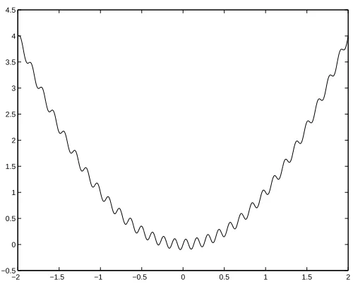
−2 −1.5 −1 −0.5 0 0.5 1 1.5 2 −0.5 0 0.5 1 1.5 2 2.5 3 3.5 4 4.5

Figure 2.1: A noisy function

IfB*C3D5E F is not inG , a backward difference gradient may be used: HJI,KLH BM-M/FON LH BMP L'H B8P7D5E FM D Q

The centered difference gradient is the preferred method and is always used if possible.

2.2 The Size of

R

Obviously the size of D is very important. As D becomes very small, the difference gradient

approaches the actual gradient. If D is not small enough, the difference gradient will not give a

very good estimate of the actual gradient of

L

.

Instead of being a problem, larger values of D are actually part of the solution to filtering

low-amplitude noise out of noisy objective functions. Consider the following noisy function:

LH BMSNTB5UC H Q V M-WXJY H V[Z\ BM Q (2.2)

In this example,

L]^H BM_N`B U and a H BMN H Q V MbWXcY H VdZ\

BM . Figure 2.1 is a graph of

LH BM .

Because of the noise in this problem, accurate gradient information can lead our optimization algorithm the wrong way. If the initial iterate is on the wrong side of one of the small oscillations,

the descent direction could very easily point away from the global minimum at Be>Ngf . Even if

the descent direction is the right one, the algorithm will likely become trapped in one of the local

minima before it reachesB e Nhf .

However, if we use a difference gradient with a relatively largeD , we can ignore the low-level

noise. By using a grosser approximation to the gradient, we effectively filter out the relatively

small effect of a

H

BM . Take, for example,B5ijNkP

Q

lmZ

andDnN

Q

omZ

. The centered difference gradient

I,KL'H

B5ipM is P

o

Q

V

, which makes the descent direction positive and fairly large. This means the

(10)

10 CHAPTER 2. NOISY PROBLEMS AND IFFCO

Obviously, we will not get a very good solution if we leave r sutwvmx in subsequent iterations.

It has served its purpose in letting the iteration move towards the global minimum, but once we

get in the neighborhood of yz , the large r will only cause problems. We would like to have an

increasingly accurate gradient as the iteration progresses and (hopefully) gets closer and closer to the global minimum.

The solution is to let r go to zero as the iteration progresses. We choose a sequence of r|{ , for

instance,

r|}~sktxpr|{s r|{

v

t

Implicit Filtering is an optimization algorithm for noisy functions based on the idea of filtering

out noise by changingr as the iteration progresses. It is very similar to Algorithm 2 with difference

gradients. r is reduced, i.e. r|{ is replaced byr|{ , when one of three things happens:

1. The linesearch fails.

2. More thanqmy iterations are taken.

3. The new termination criterion, based on the size ofr , is met. This criterion is:

, y

?

r

for some

T

.

Algorithm 3 summarizes Implicit Filtering.

2.3 IFFCO

(11)

2.3. IFFCO 11

Algorithm 3 Implicit Filtering Pick5 .

Set55 ,, , and | .

Calculate¡¢5¤£ and¥*¦¡¢5¤£ .

while¨§`5©ªc« do

while ¬¥,¦¡¢!5¤£d¬%®5 and °¯`±q²m do

Calculate the descent direction,³1´µ·¶¸

¥,¦d¡¢!5¤£.

for±¹jb±©h²m do

Letº°hº|» .

ifº satisfies (1.5) then

Exit for loop.

else if±¹±©h²m then

Signal failure; reduce and go to the next iteration of the outer while loop.

end if end for

Set¼½5´7º5³ .

Calculate¡¢!5¤£ and¥*¦¡¢5¤£ .

Update the model Hessianµ* using either the BFGS (1.9) or SR1 (1.10) update.

Set5T¼ .

Set8¿¾À .

end while Setn

¦Á

(12)

Chapter 3 Application of IFFCO to Optimization of

Natural Gas Pipelines

The natural gas used in our homes and businesses is usually transported through a highly devel-oped system of cross-country pipelines [7]. A schematic diagram of a simplified gas transmission network is shown in Figure 3.1. At points in the network, part of the gas (usually estimated at three to five percent [2]) is burned to drive engines at compressor stations. These compressors pressurize the gas in order to drive it through the pipeline. The cost of the gas used to power the compressors accounts for 25 to 50% of a typical gas transmission company’s operating budget [7]. At 1998 U.S. prices, the cost of the gas burned in this fashion was about two billion dollars per year [2]!

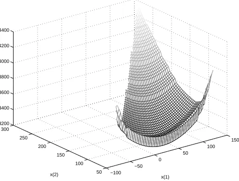
It is not surprising, then, that a common optimization problem in the industry is, given the supply and delivery flows, to minimize the amount of gas burned by the compressors. I applied IFFCO to three problems of this type. Figures 3.2, 3.3, and 3.4 show the problems, which will be referred to, respectively, as Problems A, B, and C. The vertical axis is the amount of gas (in thousand cubic feet per day) used for fuel in a compressor station. The horizontal axes are two flow variables. The flow variables may be inlet or outlet flows or a Kirchoff Law representation of possible flow splits between alternative paths.

Evaluating the objective function for a combination of the flow variables involves optimizing pressure settings throughout the network to achieve those flows. This is accomplished by solving a large combinatoric problem using non-sequential dynamic programming [2]. For some flow settings, this problem does not have a solution and the objective function will fail to return a value.

Figure 3.1: Schematic of a Simple Gas Transmission Network [7]

(13)

13

−300 −200

−100 0

100 200

300

−200 −100 0 100 200 300 3000 4000 5000 6000 7000 8000

x(1) x(2)

Figure 3.2: Problem A

−100 −50

0 50

100 150

50 100 150 200 250 300 3200 3400 3600 3800 4000 4200 4400

x(1) x(2)

(14)

14CHAPTER 3. APPLICATION OF IFFCO TO OPTIMIZATION OF NATURAL GAS PIPELINES

−100 −50

0 50

100 150

200

2 2.5 3 3.5 4 4.5 4000 4500 5000 5500 6000 6500

x(1) x(2)

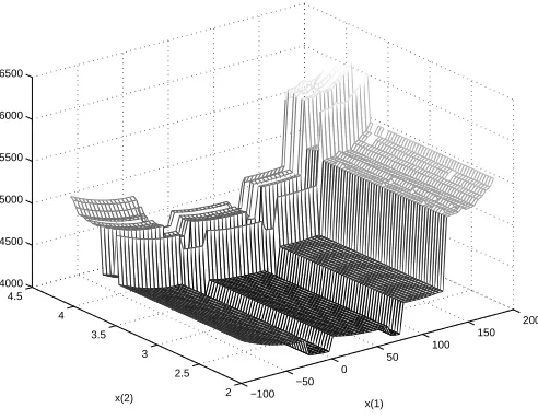
Figure 3.4: Problem C

This is the case in Figures 3.2, 3.3, and 3.4 in areas over which no surface is plotted. This situation is discussed in more detail in Chapter 4.

The discrete variables embedded in these problems give rise to some of the discontinuities in the landscapes [4]. The realities of the compressor stations themselves lead to more. The compressor stations consist of from one to more than twenty compressors. Sometimes the compressors are of different types installed over the years. Even when they are of identical manufacture, they rarely operate with the same characteristics, due to uneven wear and tear over the years [1]. The compressors can be turned on and off in different combinations.

The discontinuities of Problems A (Figure 3.2) and B (Figure 3.3) are probably due to individ-ual compressors in stations turning on and off and the discontinuous controls for certain types of engines. The discontinuities of Problem C (Figure 3.4) are likely caused by the fact that shutting down and restarting a station can cost as much as running it for several hours.

(15)

Chapter 4 Hidden Constrants

The problems I studied contained hidden constraints, and this posed a problem for IFFCO. In this chapter, I describe hidden constraints, how they appear in these problems, and what problems they present for IFFCO. Then I present two ways of dealing with hidden constraints.

4.1 Definition

Recall that the goal of a constrained optimization problem is to minimize a functionÂ in a domain

ÃuÄ`ÅÇÆ

. IFFCO finds local minimizers for such problems. A local minimizer isÈÉËÊ

Ã

such that

ÂÌ!È ÉpÍ~Î

ÂÌÈ

Í for all È½Ê

Ã

nearÈ

É

The constraints on the domainÃ

can be given as simple bound constraints, non-linear constraints, or hidden constraints. Simple bound constraints give a rectangular area in

ÅÇÆ

. The general form of simple bound constraints is

ÏmÐ Î È Ð ÎÑ Ð/ÒÔÓÕÖmÒ×ÒØØØ^ÒÙ

Non-linear constraints bound the values of at least one of the components ofÈ by a non-linear

equation. An example of a non-linear constraint on ÌÈ

Í=Ú in Å Ú is Û Î ÌÈ ÍÔÜÎ Ö ÌÈ Í Ú Ü Î ÌÈ Í=ÚÎ Ö

The constraints on

Ã

are not always known. In this case, they are called hidden constraints. Hidden constraints may be simple bound constraints or non-linear constraints, or they may not conform to any rule which is easy to write down. The only thing to do in a domain with hidden

constraints is to try evaluating the objective function Â at a point È . If Â returns a value at È , È

is in the domain and is called a feasible point. Otherwise, È is not in the domain and is termed

infeasible.

Importantly, hidden constraints can be discontinuous. This means it is not safe, in general,

to assume Â is defined everywhere between two feasible points. For example, if ÂÞÝ

Å

Ü*ß

Å

Ü

is defined at È

Õ ×

and È

Õáà

, it is not necessarily the case that Â is defined for ÈâÊäã

×Òà&å

.

(16)

16 CHAPTER 4. HIDDEN CONSTRANTS

Discovering æ to be feasible only gives limited information. It tells us that there is a (possibly

very small) neighborhood of feasible points aroundæ , but there is no way to know how large that

neighborhood is.

The problems I studied contain hidden constraints. Recall that the domain of optimization consists of values for two flow variables. Evaluating the objective function involves optimizing pressure settings throughout the system to achieve those flows. For some flow settings, this cannot be done, and the objective function fails to return a value. The combinations of flow settings for which the objective function does not return are the infeasible regions in these problems. The nature of the machinery involved makes the infeasible regions disconnected and difficult to predict. However, in the three problems I studied the feasible region was generally surrounded by a large infeasible region, and sometimes contained other, much smaller, infeasible regions. The infeasible regions are visible in Figures 3.2, 3.3, and 3.4 as areas over which no surface is plotted.

4.2 The problem with hidden constraints

Hidden constraints pose a problem for IFFCO’s method of taking difference gradients. It may happen that one or more of the points in the difference gradient stencil lie in an infeasible region. If so, IFFCO obviously cannot use the value of the objective function at that point in calculating the gradient. We would still like to use the information IFFCO has, i.e. the values of the objective function at feasible points on the stencil, to calculate something like a difference gradient which will let IFFCO avoid the infeasible region and hopefully move towards the minimum. When there are no infeasible points on the stencil, IFFCO should act normally.

4.3 Method 1

One simple solution, which I will call Method 1, is to set the objective function in infeasible regions to an artificial value greater than any expected function value. This will cause the difference gradient to point into the infeasible region, and the linesearch direction to point away from the infeasible region (remember that the line search direction is, roughly speaking, the opposite of the gradient).

Method 1 is easy to implement, and it accomplishes the goal of keeping IFFCO away from the infeasible regions. Unfortunately, using an artificially high value can make the gradient too large. The linesearch will start far away from the current iterate, possibly even in another infeasible region! Even if the linesearch starts in a feasible region, it could take many function evaluations to find a point which meets the sufficient decrease requirement, especially if the current iterate is near the minimum.

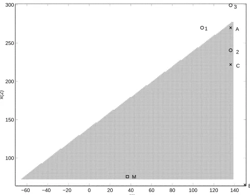
Figure 4.1 shows how Method 1 might go to an undesirable point in problem B. The graph shows the domain of the objective function. The gray region is feasible; the white region is in-feasible. IFFCO’s initial point is the point marked A, and point M is the function’s minimum. To calculate the difference gradient, IFFCO samples the objective function at points 1, 2, and 3.

Because the function is infeasible at points 1 and 3, it is assigned a value of ç[èêé at these points.

(17)

4.4. METHOD 2 17

−60 −40 −20 0 20 40 60 80 100 120 140 100

150 200 250 300

x(1)

x(2)

1

2 3

A

B C

M

Figure 4.1: Behavior of Methods 1 and 2

The difference gradient IFFCO calculates using these function values points up and to the left,

and its norm is ëíìïîíð[ñóòô . IFFCO’s linesearch direction, which is the opposite of the gradient,

points down and to the right. Because the gradient is so large, IFFCO’s linesearch direction is the projection of the opposite of the gradient onto the domain boundary. The first point the line search tries is point B, in the lower right corner of the domain. B is away from the minimum and in an infeasible region; clearly it is not a desirable point. In this case, the line search’s sufficient decrease condition prevents IFFCO from accepting B as the new point, since the reported function value at B (ð[õêö ) is much larger than at A. However, IFFCO must still waste several function evaluations in

the line search to discover its mistake.

Table 4.1: Function values for Method 1 in Figure 4.1

Point Function Value

A ÷|ìwømùêômñSò3ø

1 ðmìïõmñ~ò7ô

2 ÷|ìúðømõmñSò3ø

3 ðmìïõmñ~ò7ô

B ðmìïõmñ~ò7ô

4.4 Method 2

A better way to deal with infeasible points is to assign them the largest function value at any feasible point on the stencil. I will call this Method 2. This method also gives IFFCO a push away from the infeasible region, but now the push is proportional to the size of the function near the current iterate.

(18)

18 CHAPTER 4. HIDDEN CONSTRANTS

feasible point on the stencil occurs at point A, so this value is used for the infeasible points 1 and 3. Table 4.2 lists the function values Method 2 gives at the four points on the stencil.

Using these values, IFFCO calculates a much smaller difference gradient than with Method 1. The horizontal component of the gradient is zero, since the perceived difference in function values between A and 1 is zero. This means the linesearch direction is straight down. Since the norm

of the gradient is much smaller (ûmüwýêþmÿ compared to íüíû[ÿ for Method 1), the linesearch

step is shorter, and the linesearch moves to point C. This point has several advantages over B, the point Method 1 found. Since the function at C is smaller than at A, the linesearch only takes one function evaluation. Point C is in the feasible region, so on the next step IFFCO can use three feasible points in calculating the difference gradient, instead of the two it had to work with at the initial iterate. Also, C is in the direction of the minimum, instead of off to the right of the domain.

Table 4.2: Function values for Method 2 in Figure 4.1

Point Function Value

A |ümýmÿ

1 |ümýmÿ

2 |üúûmþmÿ

3 |ümýmÿ

C íüíû[ÿ

4.5 Comparison of Methods 1 and 2

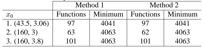
Tables 4.3, 4.4, and 4.5 compare the results of using Methods 1 and 2 on Problems A, B, and

C. The tables show the initial iterate ( ), number of function evaluations (“Functions”), and the

minimum IFFCO found (“Minimum”) for each problem. In each table, the first initial iterate is the center of the domain for that problem. The other initial iterates are near the edge of the feasible region, where the problem with hidden constraints is most likely to occur.

Method 2 is not superior in every case. In Problem A especially, Method 2 sometimes took significantly more function evaluations to find the same minimum as Method 1 (although in exam-ple 2, it interestingly found a better minimum. In this case the extra function evaluations may be justified). In other cases it is only faster, if at all, by one or two function evaluations. In still other cases, it is clearly superior: on Problem B, Method 2 converged about 12.5% faster in example 1 and about 25% faster on example 3.

It is somewhat unfair to compare the two methods in this way. Methods 1 and 2 follow different iteration histories when they encounter infeasible points. That can significantly effect how long IFFCO takes to find a minimum and what minimum it finds, just as choosing different initial iterates can sometimes drastically change the number of function evaluations or the minimum found. Method 2 protects IFFCO from a possibly costly error, and if it does not always converge

faster than Method 1, it at least does not converge much slower. Therefore we chose to use Method

(19)

4.5. COMPARISON OF METHODS 1 AND 2 19

Table 4.3: Comparison of Methods 1 and 2 in Problem A

Method 1 Method 2

Functions Minimum Functions Minimum

1. (0, 27.5) 55 3271 55 3271

2. (-150, 150) 72 3271 92 3242

3. (150, -50) 71 3269 77 3270

4. (100, 200) 79 3235 85 3235

Table 4.4: Comparison of Methods 1 and 2 in Problem B

Method 1 Method 2

1. (40, 182.5) 72 3208 63 3208

2. (100, 160) 62 3208 62 3208

3. (140, 75) 69 3208 52 3208

Table 4.5: Comparison of Methods 1 and 2 in Problem C

Method 1 Method 2

1. (43.5, 3.06) 97 4041 97 4041

2. (160, 3) 63 4063 62 4063

(20)

Chapter 5 Computational Experiments

In this chapter I describe the computational results we achieved by running IFFCO on Problems A, B, and C.

5.1 IFFCO Parameters

IFFCO has a number of parameters which must be “tuned” for use with each problem. IFFCO will generally perform “ok” with the default values for these parameters. However, IFFCO’s perfor-mance, measured in terms of the number of function evaluations and the how small the minimum it finds is, can be improved by changing the parameters. Since these problems were very simple, I was able to run IFFCO multiple times on each problem to determine which parameter settings worked best. The best parameters for each problem are not necessarily the same. Since the goal was to find parameters that work in general for this class of problems, I used the parameters that seemed to give the best performance, on average, on all three problems.

Since the choice of an initial iterate can greatly affect IFFCO’s result, I set equal to the

center of the bounding box in each problem in order to be able to compare the results across problems. Table 5.1 lists the “best” parameters I found for IFFCO on these problems. The IFFCO runs described in the next section all used these parameters. For a full explanation of what each parameter means, see [5].

A couple of examples will illustrate the type of impact the choice of these parameters can have, as well as the way I made choices about what parameters to use.

First, consider selecting , the smallest value of used. Too large a value can cut off the

algorithm before it gets very close to the minimum; too small a value can cause the algorithm to waste function evaluations for very small improvements in the objective function value. I tried

equal to ! , " $# , and "$ % . Table 5.2 shows the results of this experiment for each

problem.

Reducing&' to" $# significantly reduced the minimum found in Problems A and B, at the

cost of more function evaluations. Further decreasing&' substantially increased the number of

function evalations but did not make the minimum much better. I decided to set&')(* $# .

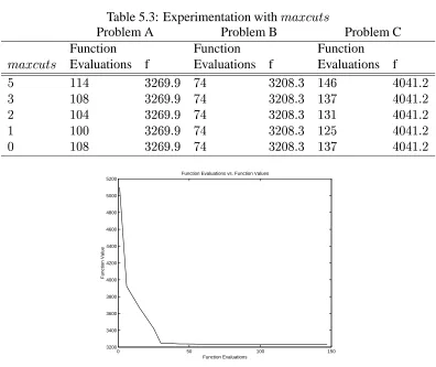
Now consider the task of selecting an appropriate value for,+-/.103254 , the number of reductions

in the step length before the linesearch signals failure. I experimented with,+6/.103254 equal to , ,

7

, and8 . The results are tabulated in Table 5.3

(21)

5.2. RESULTS USING IFFCO 21

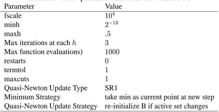
Table 5.1: “Best” parameter values for use with IFFCO

Parameter Value

fscale 9:<;

minh =->3?A@

maxh BC

Max iterations at each D E

Max function evaluations) 9:6:6:

restarts :

termtol 9

maxcuts 9

Quasi-Newton Update Type SR1

Minimum Strategy take min as current point at new step

Quasi-Newton Update Strategy re-initialize B if active set changes

Table 5.2: Experimentation withFGH'D

Problem A Problem B Problem C

Function Function Function

FGH'D Evaluations f Evaluations f Evaluations f 9": > @ CI E6=6J:KBJ6C L$J E-=:MKBE IL L6:L$=NB:-J 9": >$; 969L E6=O6IKBI J<L E-=:MKBE 9L-O L6:LP96BQ9"I 9": > R 9SCO E6=O6IKBM 9S=N9 E-=:MKBE 9SJ6= L6:LP96BQ9"M

One can see that increasing F,T6U/VXW3Y5Z beyond 9 resulted in little or no improvement in the

minimum found and increased the number of function evaluations. F,T6U/VXW3Y5Z\[]9 actually saved

function evaluations overF,T6U/VXW3Y5Z^[_: , however, so I chose to set F,T6U/V1WY5Z`[*9 .

Decisions on the other parameters were made in a similar fashion. It is possible that other parameters would give slightly better results, or require slightly fewer functions, but it is unlikely that the difference would be significant.

5.2 Results Using IFFCO

On Problem A, IFFCO found a minimum ab[cE-==MKBI6: after 9L$J function evaluations. The

con-vergence of IFFCO for this problem is plotted in Figure 5.2.

On Problem B, IFFCO found a minimuma,[dE-=<:6MKBE6: inO6O function evaluations. The

conver-gence of IFFCO for this problem is plotted in Figure 5.2.

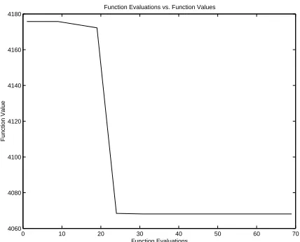
On Problem C, IFFCO found a minimum a_[]L-:6O6MNB:6I in OI function evaluations using the

(22)

22 CHAPTER 5. COMPUTATIONAL EXPERIMENTS

Table 5.3: Experimentation withe,f6g/h1ij5k

Problem A Problem B Problem C

Function Function Function

e,f-g/h1i3j5k Evaluations f Evaluations f Evaluations f l mmn o-pqrKsr t<n o6pu6vKso mn6q n-unPm6sp o mu6v o-pqrKsr t<n o6pu6vKso m"o6t n-unPm6sp p mun o-pqrKsr t<n o6pu6vKso m"oNm n-unPm6sp m mu6u o-pqrKsr t<n o6pu6vKso mSpl n-unPm6sp u mu6v o-pqrKsr t<n o6pu6vKso m"o6t n-unPm6sp

0 50 100 150

3200 3400 3600 3800 4000 4200 4400 4600 4800 5000 5200

Function Evaluations vs. Function Values

Function Evaluations

Function Value

Figure 5.1: Convergence of IFFCO in Problem A

5.3 A Hybrid Approach

(23)

5.3. A HYBRID APPROACH 23

10 20 30 40 50 60 70

3208 3208.5 3209 3209.5 3210 3210.5 3211 3211.5 3212 3212.5

Function Evaluastions

Function Value

Figure 5.2: Convergence of IFFCO in Problem B

0 10 20 30 40 50 60 70

4060 4080 4100 4120 4140 4160 4180

Function Evaluations

Function Value

(24)

Chapter 6 Parallel Computing

Parallel computation can offer significant speed advantages for some algorithms. Section 6.1 will explain, in a simplistic way, some of the issues of parallel computing. Section 6.2 will explain how IFFCO can be parallelized.

6.1 Overview

Most personal computers run programs in serial. This means instructions are executed sequentially, one after another. In a serial computer, only one program can run at a time. Modern operating systems create the illusion that many programs are running at once by switching rapidly from one to another.

Parallel computers execute many instructions at once by running programs on many processors. A parallel computer may be running a different program on each processor, or each processor may be running a different part of the same program. It might seem that, given a parallel machine with four processors, one could divide a program into four parts, run each part on a separate processor, and finish in one-fourth the time required for a serial implementation. In practice, things rarely work out quite so well.

To see why, consider multiplying two vectors,w andx , of length four. This requires four

mul-tiplications and three additions. On a serial computer, each operation would be done sequentially, and all together they would take seven cycles (assuming multiplication and addition take one cycle each). On a parallel machine with four processors, all the multiplications can be done at once, each

on a separate processor, in one cycle. Next, one processor can computewyzx-y6{|w}~x} while a second

processor computesw~x{w~x . This also takes one cycle. Finally, one of the processors can do

the final addition. All together, the parallel implementation requires three cycles, for a speedup of

6

. This is significant, but it is not one-fourth the time the serial version requires.

This example demonstrates several important concepts of parallel computing. First, not every part of a problem is fit to be parallelized. Sometimes, one operation depends on the result of another, as the third addition in the vector multiplication example depends on the results of the first two additions. In this case, those two parts of the problem cannot be executed in parallel with each other. When some part of an algorithm consists of operations which can be done at the same time, we say it exhibits parallelism.

(25)

6.2. PARALLELISM IN IFFCO 25

Second, throwing more processors at a problem does not always reduce the time required to solve it. If we had eight processors to run the vector multiplication on, we could do it no faster than 3 cycles, since there is no work for the four additional processors. The problem simply cannot be divided further. The number of processors a problem can be divided (or scaled) onto determines the problem’s scalability.

Third, there is the issue of load balancing. We assumed that every operation in the vector multiplication would take the same amount of time. If this is not the case, then some processors will end up waiting, with nothing to do, while another processor finishes a longer task. Load balancing strategies aim to distribute (roughly) the same amount of work to each processor so that idle processor time is kept to a minimum.

Finally, we must consider the time required for communication between processors. The paral-lel computing environments IFFCO has run on are distributed memory machines, like most of the largest parallel computing machines. This means each processor has its own private store of data. If one processor needs something another processor knows, the two processors have to communi-cate. This takes time. So it is not true that the parallel implementation of the vector multiplication would take only three cycles. There is additional overhead for communication. Communication is one of the biggest culprits in slowing down parallel computation.

There are two main standards for communication in distributed memory parallel computing environments. PVM (Parallel Virtual Machine) was the most widely used standard until a few years ago. Now, MPI (Message Passing Interface), first introduced in 1994, has largely superseded PVM. The parallel version of IFFCO uses PVM for inter-processor communications. A port of IFFCO to MPI sometime in the future is likely.

This section has presented a gloomy view of parallel computing, outlining the problems that can come up. However, parallel computing techniques can significantly reduce run times if applied properly to algorithms that are good candidates for parallelization. IFFCO is such an algorithm.

6.2 Parallelism In IFFCO

IFFCO’s basic algorithm gives us a natural way to implement parallelism. Algorithm 3 gives the serial algorithm for IFFCO. Two operations in algorithm 3 involve evaluating the objective function

multiple times:

Calculate the difference gradient

Perform a linesearch in the direction

Importantly, none of these function evaluations are dependent on the others. In other words, finding

the first function value needed to form

has nothing to do with finding the second function value, and finding the first value in the linesearch has nothing to do with finding the second. IFFCO can take advantage of this on a parallel machine by sending each function evaluation to a different processor. In the parallel implementation of IFFCO, one processor serves as the master, sending instructions to the other processors to evaluate

at certain points and interpreting the results. The

other processors are slaves; their sole job is to evaluate

(26)

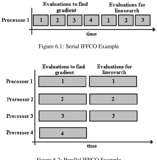
26 CHAPTER 6. PARALLEL COMPUTING

Figure 6.1: Serial IFFCO Example

Figure 6.2: Parallel IFFCO Example

6.2.1 Comparison of Serial and Parallel IFFCO

If the domain of is in ) , calculating requires from to function evaluations.

De-pending on how quickly the sufficient decrease condition is met (if it is met at all), the linesearch

can take up to¡ |¢d£6 function evaluations. So may be evaluated as many as<¥¤¦ times

in one iteration of IFFCO.

Depending on the application, evaluating can take minutes or even hours. In fact, function

evaluations often take so long compared to the rest of the work IFFCO does that the total time for one iteration of IFFCO is approximately the same as the time spent doing function evaluations.

minute. In a serial implementation of IFFCO, the function evaluations must occur one after another

Now assume<° _± processors are available to IFFCO in a parallel machine. Now the function

evaluations can be performed as in Figure 6.2. All four function evaluations for the gradient are

done at once, on four separate processors, and then combined on one processor to form .

(27)

6.2. PARALLELISM IN IFFCO 27

6.2.2 Scalability of IFFCO

Notice that at most²,³6´¶µ·<¸¶¹~²|º processors can be used at a time in this parallel implementation of

IFFCO. Allocating more than²,³6´¶µ·<¸¶¹~²|º processors to IFFCO will not speed up its performance;

the extra processors will remain idle.

In practice, we usually run IFFCO on»½¼_¾ processors, where» evenly divides¸ . This means

the function evaluations for the difference gradient (remember that there are between ¸ and ·¸ of

them) can be fairly evenly distributed between the processors. The extra processor is the master processor.

More processors can be utilized and performance further increased if the calculation of¿ itself

has some sort of parallelism. In this case, each slave processor controls other slave processors

which each do part of the work of evaluating¿ .

6.2.3 Load Balancing in IFFCO

The preceding discussion has oversimplified several points for the sake of explanation. One of them is the assumption that each function evaluation takes the same amount of time. In the real

world, the time it takes to evaluate¿µ´º can vary greatly depending on´ . For instance,´ could be

a vector of parameters, such as damping constants, passed to an ODE solver to simulate a system involving springs. Depending on the damping constants, the system could take a very short or very long time to solve.

Further, we generally don’t have the luxury of one processor per evaluation of¿ . This, plus the

difference in time between evaluations of¿ , leads to load balancing problems in IFFCO.

As a specific example, take the task of calculating ÀÁS¿µ´º on two processors using four

func-tion values: ¿µ´ÂÃº ,¿µ´Ä1º ,¿µ´ÅXº , and¿µ´3ÆÇº . We might first think of dividing the work like this:

Processor 1 Processor 2

¿µ´ÂÈº ¿µ´ÅXº ¿µ´ÄXº ¿µ´3ÆÇº

This strategy is simple, but naively assumes that all four function evaluations take the same

amount of time. Suppose, instead, that ¿µ´ÂÈº takes three times as long as the others to evaluate.

The situation is depicted in Figure 6.3. In this scenario, Processor 2 could have evaluated ¿µ´ÅÉº ,

¿µ´3ÆÇº , and ¿µ´Ä1º in the time it took Processor 1 to evaluate just¿µ´Â5º. Furthermore, Processor 2 is

idle half the time. This is a pessimistic case, but it can arise and IFFCO’s strategy for distributing

¸ function evaluations toÊ processors is designed to guard against it. This strategy is given as

Algorithm 4.

Algorithm 4 Distribute

Distribute the first¸ points to processors¾ËÌËË&Ê

while There are points left do

(28)

28 CHAPTER 6. PARALLEL COMPUTING

Figure 6.3: Bad Load Balancing

Figure 6.4: Good Load Balancing

Algorithm 4 changes the situation in Figure 6.3 to that in Figure 6.4. The time required is one minute less, and Processor 2 is no longer idle half the time. Of course, the timings won’t normally work out so neatly.

In the case that all the function evaluations take about the same time, this strategy does what

our intuition suggested at the beginning: it distributes (approximately)ÍÎXÏ function evaluations to

(29)

Bibliography

[1] R.G. Carter. Compressor station optimization: computational accuracy and speed, 1996.

[2] R.G. Carter. Pipeline optimization: dynamic programming after 30 years. Proceedings of the Pipeline Simulation Interest Group, Paper number PSIG-9308, 1998.

[3] R.G. Carter, J.M. Gablonsky, A. Patrick, C.T. Kelley, and O.J. Eslinger. Algorithms for noisy problems in gas transmission pipeline optimization. Not sure, 2000.

[4] R.G. Carter, D.W. Schroeder, and T.D. Harbick. Some causes and effect of discontinuities in modeling and optimizing gas trnasmission networks. Proceedings of the Pipeline Simulation Interest Group, Paper number PSIG-9308, 1994.

[5] Tony Choi, Paul Gilmore, Owen J. Eslinger, C.T. Kelley, Alton Patrick, and Jorg Gablonsky. Iffco: Implicit filtering for constrained optimization, version 2. Technical Report CRSC-TR99-23, North Carolina State University, Center for Research in Scientific Computation, 1999.

[6] C.T. Kelley. Iterative Methods for Optimization. Society for Industrial and Applied Mathe-matics, Philadelphia, 1999.

[7] C.A. Luongo, B.J. Gilmour, and D.W. Schroeder. Optimization in natural gas transmission networks: a tool to improve operational efficiency. Presented at the 3rd SIAM Conference on Optimization, 1989.

Implicit filtering for constrained optimization and applications to problems in the natural gas pipeline industry