Approved by:

(1)

WATER SUPPLY AND WATER QUALITY: PUTTING TOGETHER HOW NATURAL AND HUMAN FACTORS AFFECT THESE, USING SATELLITES

Mejs Hasan

A dissertation submitted to the faculty at the University of North Carolina at Chapel Hill in partial fulfillment of the requirements for the degree of Doctor of Philosophy in the Department of Geological

Sciences in the College of Arts and Sciences.

Chapel Hill 2018 Approved by: Larry Benninger Aaron Moody John Bane Colin West Xiaoming Liu

(2)

(3)

iii

ABSTRACT

Mejs Hasan: Water supply and water quality: Putting together how natural and human factors affect these, using satellites

(Under the direction of Larry Benninger and Aaron Moody)

This dissertation explores the interplay of human and natural factors upon water resources in the Chesapeake Bay, the Tigris and Euphrates Rivers, and the marshes of southern Iraq. I used high-quality but expensive-to-collect fieldwork data of water status. I combined that data with regularly-produced satellite images covering large sections of the earth. Combining high-quality fieldwork data with global, continuous satellite data can produce datasets that are richer than the sum of their two parts.

I first studied the effect of storms on water quality in the Chesapeake Bay by using a relationship between satellite-measured red light reflectance and ground measurements of total suspended solids (TSS). This resulted in viable reflectance-TSS relationships for five major Western Shore rivers. Modeling a single reflectance-TSS relationship for the entire estuary produced poorer models with less significance compared to treating each channel separately. After studying the aftermath of 2800 rain events, I found some evidence that higher rainfall corresponds to a lower distribution of TSS concentrations one day following the storm in forested, compared to urban, watersheds.

In chapter 2, I studied how conflicts and drought disrupt water supply on dams and barrages along the Tigris and Euphrates rivers. I used a satellite-based algorithm, the normalized difference water index (NDWI), to monitor changes in the extent of surface reservoirs (1985-present). The most sudden changes in water supply occurred during conflict, but conflict was not often a cause of the greatest absolute changes to reservoir area. In chapter 3, I again used NDWI and similar algorithms to examine how the seasonal cycle of marshes at the southern end of the Tigris and Euphrates has been affected by

(4)

iv

drought, development, and conflict. I found some evidence that the yearly timing of the marsh peak size has become more variable after exposure to these stressors.

No matter the stressor – from storms to drought to war – water quality and supply are highly affected by human and natural factors. In combination with ground information, satellite data can fill in data gaps and offer further insights.

(5)

v

I dedicate my dissertation to the three UNC-Chapel Hill and N.C. State students killed in 2015: Yusor Mohammad Abu-Salha, her sister Razan Mohammad Abu-Salha, and her husband Deah Shaddy Barakat; and to our former student body president, Eve Marie Carson, killed in 2008.

I also dedicate it to the many humanitarian workers who traveled to Iraq or neighboring countries in order to build hospitals, set up voting systems, or support education of girls, and instead were killed.

Also, this dissertation is dedicated to the many Iraqi children who have died or suffered through the last three decades of war.

(6)

vi

ACKNOWLEDGEMENTS

This work was supported and funded by the Graduate School at the University of North Carolina at Chapel Hill (UNC-CH), Royster Society of Fellows, the Department of Geology at UNC-CH, and the Martin Funding Program at the Department of Geology.

I was supported through this process by my terrific advisors, Dr. Larry Benninger and Dr. Aaron Moody, as well as Dr. John Bane, Dr. Colin West, and Dr. Xiaoming Liu who comprised the rest of my committee. They helped me out of very hard situations, heedless of the extra time and work it meant for them. They were patient, excited about my progress, and devoted many conversations to moving the research forward. Their support meant that I was able to successfully complete my degree, and to experience the amazing opportunities that fell into my lap over the past few years. I have always appreciated that my entire committee never hesitated for a second when I asked them for help, that they always showed a lot of confidence in me, and that they always focused on the good. Thank you.

The support from the Royster Society of Fellows – Sandra Hoeflich, Teresa Phan, Jennifer Gerz-Escandon, Marsha Collins – was also so wonderful and so appreciated.

This study was possible due to governmental and institutional support for open access to

environmental data. The satellite data on which this dissertation depended so heavily were freely acquired from American government servers. Specifically, Chesapeake Bay MODIS data was retrieved from the Level-1 and Atmosphere Archive & Distribution System (LAADS) Distributed Active Archive Center (DAAC), located in the NASA Goddard Space Flight Center in Greenbelt, Maryland. Landsat and ESA images of the Middle East were retrieved from Google Earth Engine servers, to which the satellite images have been uploaded, processed, and corrected by NASA and the U.S. Geological Survey. Other sources of

(7)

vii

freely available data used include the Chesapeake Bay Program, NOAA rain gages, and USGS discharge stations.

UNC-CH libraries also played a central role by offering statistical consulting help (especially Chris Wiesen in Davis Library), providing access to books and journals, and procuring old and difficult-to-locate reports which were especially key for chapter 2.

Ron Vogel of NOAA provided a very helpful review of the portions of the dissertation dealing with the Chesapeake Bay, and Ali Hasan of IBM provided statistical insight on the same chapter. Helpful email communications and documents from Nadhir Al-Ansari of Luleå University of Technology gave great insight and needed information on Mosul Dam for chapter 2. I thank them all for their help.

Finally, thank you to all the family, friends, and relatives who took an interest in my research and whose good wishes sped me along.

(8)

viii

LIST OF TABLES

Table 1. NOAA rain gages. ... 14

Table 2. Model parameters. ... 20

Table 3. Accuracy analysis. ... 22

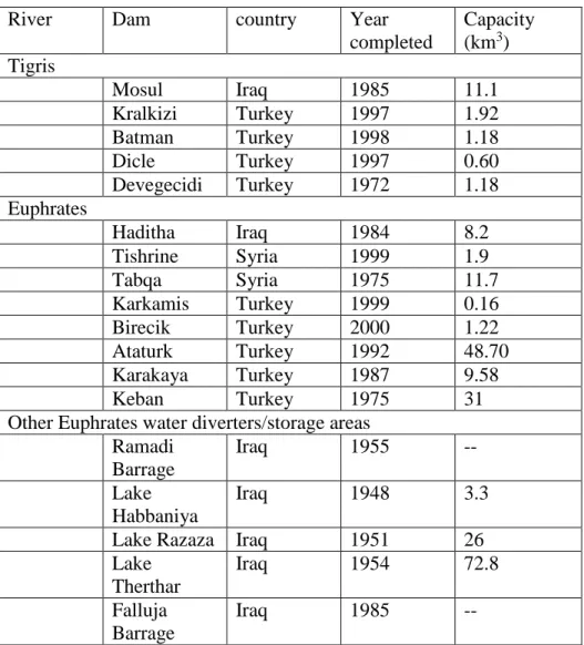
Table 4. Dams and barrages along the Tigris and Euphrates. ... 38

Table 5. Tigris/Euphrates error matrix and accuracy results. ... 47

Table 6. Summary of substantial changes in water supply along the Tigris and Euphrates. ... 50

Table 7. Correlations between dam lake sizes. ... 55

Table 8. Different periods of marsh surface area size. ... 73

Table 9. Correlations between upstream reservoirs and Hawiza marsh area. ... 83

Table S1. List of conflicts. ... 116

(12)

xii

LIST OF FIGURES

Figure 1. Chesapeake Bay study area. ... 6

Figure 2. Satellite reflectance-TSS concentration relationships. ... 18

Figure 3. Chesapeake TSS time series. ... 20

Figure 4. TSS estimates derived from MODIS. ... 25

Figure 5. Box-plots of post-storm TSS estimates. ... 28

Figure 6. Peaks in the MODIS-derived TSS estimates. ... 30

Figure 7. MODIS-derived TSS estimates following high rainfall. ... 33

Figure 8. Map of the Tigris/Euphrates study area. ... 41

Figure 9. The head of Mosul Dam illustrated in Landsat 8 imagery. ... 43

Figure 10. Surface area of Haditha (a) and Mosul (b) reservoirs. ... 48

Figure 11. Rates of change in reservoir lake-area of Haditha (a) and Mosul (b) reservoirs. ... 51

Figure 12. Scatterplots of reservoir size. ... 56

Figure 13. A map and a conceptual diagram of the marshes in southern Iraq. ... 67

Figure 14. Marsh error analysis. ... 72

Figure 15. Timeline of the total marsh surface area. ... 74

Figure 16. Landsat images of the marshes. ... 77

Figure 17. The range of marsh extent by month. ... 79

Figure 18. Timing of marsh peak and minimum extent. ... 80

Figure 19. The monthly extent of vegetated and open water marsh area... 81

Figure 20. The yearly ratio of the peak vegetated marsh area to minimum marsh area. ... 82

Figure S1. Percent of various land covers for the 12 gage-station sites in the Chesapeake Bay; ... 93

Figure S2. Significance of the reflectance-TSS models... 94

Figure S3. Reflectance-TSS relationships for Mainstem stations. ... 95

Figure S4. CBP measures of TSS concentrations versus MODIS-derived estimates. ... 97

(13)

xiii

Figure S6. Cumulative precipitation based on PERSIANN estimates, 1983-2016. ... 99

Figure S7. Distribution of dates with satellite data by month and by year, for Mosul reservoir. ... 100

Figure S8. NDWI distributions for land and reservoir polygons. ... 102

Figure S9. Geographical position of points used in validation analysis. ... 103

Figure S10. Altimeter-Landsat scatterplots. ... 104

Figure S11. Close-ups of significant episodes of lake surface area. ... 106

Figure S12. Close-ups of significant episodes of lake surface area. ... 108

Figure S13. Images representing changes in Mosul and Haditha reservoirs. ... 110

Figure S14. Floods in near Abu Ghraib. ... 111

Figure S 15. Median monthly temperatures in the Tigris/Euphrates. ... 112

Figure S16. The discharge at Kut, Iraq. ... 113

Figure S17. The month during which Hawiza marsh has its peak area of open water, by year. ... 114

(14)

xiv

LIST OF ABBREVIATIONS

CBP Chesapeake Bay Program

CDOM Colored dissolved organic matter

DAAC Distributed Active Archive Center

ETM Estuarine turbidity maximum

ETM+ Enhanced Thematic Mapper Plus

LAADS Level-1 and Atmosphere Archive and Distribution System

GRACE Gravity Recovery and Climate Experiment

HUC Hydrologic unit codes

MODIS Moderate Resolution Imaging Spectroradiometer

NDVI Normalized difference vegetation index

NDWI Normalized difference water index

NIR Near-infrared

OLI Operational Land Imager

PERSIANN Precipitation Estimation from Remotely Sensed Information using Artificial Neural Networks

RIM River-Input Monitoring

RMSE Root mean square error

SAV Submerged aquatic vegetation

SeaWiFS Sea-viewing Wide Field-of-view Sensor

(15)

xv

TOA Top-of-the-atmosphere

TM Thematic Mapper

TSS Total suspended solids

(16)

1

INTRODUCTION

Availability of clean water is expected to be one of the most important issues faced by 21st century society. The Millennium Ecosystem Assessment (2005) suggests that use of fresh water for drinking, industry and irrigation has reached unsustainable levels, and particularly in the Middle East, a full third of all water-use is sourced unsustainably. Such precarious water sources become even scarcer during droughts and other environmental variability. For example, the Middle East underwent its most severe drought on record between 2007 and 2009 (Trigo et al. 2010), and it is believed that the current Syrian Civil War was in part driven by the drought-linked agricultural decline (Kelley et al. 2015). As the conflict spread to neighboring Iraq, water has often been used as a weapon of war (Collard 2014). Closer to home, the Chesapeake Bay and other coastal ecosystems face challenges in preserving water quality to sufficient standards to meet ecosystem and recreational needs, while also allowing room for upstream development activities and land-use (Aighewi et al. 2013).

Satellite remote sensing is a valuable tool for studying and addressing these issues. For example, the extent of marshes at the confluence of the Tigris and Euphrates rivers has been mapped by three generations of Landsat satellite data over a 30-year time period (Al-Handal & Hu 2014, Becker 2014, Ghobadi et al. 2015). Trends in groundwater data in the Middle East have been described using GRACE satellite data (Voss et al. 2013, Tourian et al. 2015). In the Chesapeake Bay, color reflectance properties of various water constituents have been analyzed and can yield models describing suspended sediment concentrations (Tzortziou et al. 2007).

In this dissertation, I use remote sensing and ground data to investigate changes in water supply and quality caused by human-driven use change and by human conflict. First, I investigate how land-use, such as farms and urban areas, plays a role in determining suspended sediment levels in the

(17)

2

supply in Tigris/Euphrates basin has changed over the last three decades, both as a reaction to conflicts and to development (chapter 2 and 3).

The Chesapeake Bay is the nation’s largest estuary, home to one of its most productive ecosystems, and is an icon of American heritage and history (Kemp et al. 2005). Nutrient and total suspended solid (TSS) concentrations have exceeded Clean Water Act regulations in recent decades, resulting in sediment-driven water clarity impairment and light attenuation. How storms affect TSS concentrations is still not well-understood, since studies are usually small in scope and give conflicting results (Ward 1985, Gellis et al. 2009, Sutton et al. 2009). This can be analyzed in further depth by using satellite-derived reflectance properties of total suspended solids (TSS) in the Bay in order to estimate TSS concentrations. Such relationships enable us to estimate TSS over longer time intervals and at more locations than is possible from fieldwork. Some such relationships have already been published, but there is room for improvement. Current relationships are limited to a narrow TSS concentration range, so very high or very low values cannot be estimated. Also, relationships devised for the Chesapeake Mainstem are extrapolated to all tributaries of the Bay, regardless of whether separate tributaries may have

individual sediment signatures with different reflectance properties (Tzortziou et al. 2007, Ondrusek et al. 2012, Son & Wang 2012, Zheng et al. 2015).

Aspects of Tigris/Euphrates basin water resources have also been studied via remote sensing. For example, the effects on vegetation of both a 1998-2000 and a 2007-2009 drought have been examined using the satellite-derived normalized difference vegetation index (NDVI) (Trigo et al. 2010, Villa et al. 2014). Water level estimates for major lakes and reservoirs in this region also exist through satellite altimeters, and show how water levels recede in response to drought (Trigo et al. 2010, Voss et al. 2013, Joodaki et al. 2014). How conflict and development intertwine with drought and affect water supply has not been studied.

This dissertation consists of three chapters:

Chapter 1: Study of how storms and land-use affect TSS concentrations in the Chesapeake Bay using satellite reflectance properties. The Chesapeake Bay has an impressive monitoring program

(18)

3

that has sampled the Bay for TSS since 1986, but many gaps in time and space exist. I looked for relationships between red light reflectance (measured by satellite) and total suspended solid

concentrations (measured from a boat) in order to fill in these gaps. Red light reflectance is retrieved from the Terra sensor on the NASA satellite MODIS. I assessed whether Chesapeake tributaries are better served by their own reflectance-TSS relationships, rather than reliance on a single Bay-wide model; used these relationships to greatly expand post-storm TSS estimates in the Chesapeake and address the ambiguity in current studies on how storms affect TSS; and evaluated whether different land-uses affect the storm-TSS patterns. I found that post-storm river TSS is higher in urban and agricultural areas compared to forests.

Chapter 2: Investigate how the different and at-times coupled impacts of drought, war, and water management have affected both quantity and quality of water resources in the

Tigris/Euphrates area. I used altimeter-derived measures of water depth in lakes and reservoirs, and

Landsat-derived water surface area measurements (via the normalized difference water index algorithms), in order to create timelines of water supply behind dams and in rivers. I also used globally compiled datasets of precipitation and temperature, and Landsat-derived upstream reservoir surface area in order to control for rainfall and snowmelt, upstream dam management, and evaporation. Combining all this information in a crude model, I studied if anomalous changes in reservoir surface area occur during battles and wars. I found that conflict did produce some very sharp changes in reservoir surface area, though not all conflict did; drought also produced large changes, though at a slower pace.

Chapter 3. Investigate how coupled human-natural factors have affected the southern marshes on the Tigris/Euphrates in terms of the seasonal patterns. I developed satellite-based

monthly surface area trends of the Tigris/Euphrates southern marshes. From these, I determined the seasonality in marsh lakes, and quantify when the ‘wet season’ occurs and how the onset and duration of this season is affected by upstream dam development and/or drought. I also determined the difference in the marsh extent during the dry versus wet seasons. I found some evidence that the difference in marsh

(19)

4

extent between the peak and minimum seasons is declining, and that the timing of the wet/dry seasons has become more variable.

Water is a vital resource for all forms of life, and is connected to survival, sanitation, food production, commerce, recreation, and ecosystems. Growing populations make it more difficult for competing stakeholders to meet all their needs while also preserving the environmental flows needed for biodiversity, habitats, and ecosystems. Disturbances such as storms, drought, and war can all make this competition even more acute. The research described here will increase knowledge of how water supply and some aspects of quality are affected by such disturbances. It provides information on which types of human activities are most stabilizing for water supply and quality, and which are not.

(20)

5

CHAPTER 1: RESILIENCY OF THE WESTERN CHESAPEAKE BAY TO TOTAL

SUSPENDED SOLID CONCENTRATIONS FOLLOWING STORMS AND ACCOUNTING

FOR LAND-COVER

In the first chapter of this dissertation, I discuss the use of satellite images to study certain aspects of water quality in the Chesapeake Bay. People are often surprised to learn that a satellite image can shed light on water quality, but it is due to the fact that the more impurities water contains, the more light it reflects. Satellites can detect that change in reflectance. I created relationships between satellite reflectance and total suspended solids (TSS), and then used those relationships to explore how TSS changes in the Bay following major storms. I showed that by coupling two very different datasets – high quality ground data with global and continuous satellite data – the resulting dataset is more

comprehensive than the sum of its two parts.

This paper was published as: Hasan, M., and L. Benninger. 2017. Resiliency of the western Chesapeake Bay to total suspended solid concentrations following storms and accounting for land-cover.

Estuarine, Coastal and Shelf Science 191. doi:10.1016/j.ecss.2017.04.002.

Section 1: Introduction

The Chesapeake Bay is the nation’s largest estuary, home to one of its most productive

ecosystems, and is an icon of American heritage and history (Kemp et al. 2005). It extends across a large swath of the mid-Atlantic coast, from the mouth of the Susquehanna River near Havre de Grace,

Maryland, to its juncture with the Atlantic Ocean near Virginia’s Norfolk metropolitan area (Figure 1). However, nutrient and total suspended solids (TSS) have exceeded Clean Water Act regulations in recent decades, resulting in sediment-driven water clarity impairment and light attenuation. This inhibits solar energy from reaching submerged aquatic vegetation (SAV) and oyster reefs and the associated fish nurseries, some of the most crucial components of the ecosystem (Jordan et al. 1997, Focazio et al. 1998,

(21)

6

Gellis et al. 2009). In this paper, we use satellite data to study the effect of storms and land cover on TSS levels.

Figure 1. Chesapeake Bay study area. Black squares represent the CBP stations and the extent of the

study area upstream each channel. CBP stations identified in the paper are labeled in pink. Location and name of NOAA rain gages are represented by red triangles/white text bubbles. Light blue text labels indicate channel names. Orange text labels indicate NOAA “tides and currents” stations. The lower green dash is the Virginia-Maryland border; the upper green dash is the Bay Bridge.

(22)

7

Uncoordinated research on storm-effects in the Bay has been performed in a patchwork way at limited study sites and times. Some studies found TSS and nutrients increased following storms, but this is not universal and depends on sediment size, organic/mineral content, compaction, invertebrate mucus secretions, land slope, and water velocity (Ward 1985, Gellis et al. 2009, Sutton et al. 2009). Furthermore, wet weather is not alone in increasing TSS levels, as dry, windy weather can lead to increased erosion and wave-caused resuspension acting on normally submerged river beds (Stevenson et al. 1985, Ward & Twilley 1986). Storm-induced TSS concentrations are not necessarily runoff-based but may be wind or tidal-driven bottom resuspension, particularly in areas without buffering features like SAV beds (Ward et al. 1984, Stevenson et al. 1985, Ward 1985). The settling periods for post-storm TSS levels before a return to normal conditions can be less than 24 hours for smaller events, but as high as weeks for large hurricanes (Ward et al. 1984, Stevenson et al. 1985, Liu & Wang 2014). Land cover variables, such as proximity and size of urban areas, forests, agriculture and wastewater treatment plants, play an important role in how the Bay responds to stressors (Aighewi et al. 2013). Heavily forested watersheds can sustain post-storm TSS concentration declines due to dilution if water is added more rapidly than suspended solids, while urban watersheds may become more susceptible to storm-driven TSS increases due to streambank erosion (Stevenson et al. 1985, Ward & Twilley 1986, Devereux et al. 2010).

To investigate effects of storms and land cover on TSS levels, data must be gathered directly following storms in river basins with different land cover type dominance. Such data is difficult to come by. The EPA Chesapeake Bay Program (CBP) has systematically sampled the Bay for nutrients and TSS since 1986, but tidal river measurements are often made once a month at routine station stops where the schedule does not shift to emphasize different weather conditions (Olson et al. 2012). Indeed, sampling is less likely to occur during stormy weather due to harsher conditions. Lacking data, TSS may be estimated after the fact using water quality models that rely on rainfall and hydrodynamic principles. However, a review of ten such models in the Chesapeake Bay found them afflicted with conflicting results, and that while a model might be suited to a specific river, it could not be extrapolated to the entire watershed (Boomer et al. 2013). Alternatively, the USGS and other researchers have used daily streamflow

(23)

8

monitoring to create load-flow relationships based on time, discharge, and season (Moyer et al. 2012, Zhang et al. 2015, Chanat et al. 2016).

Satellite light reflectance data provide the potential to improve both spatial and temporal coverage of surface-water TSS levels. Since the 1970s, water light reflectance models of sediment concentrations have been developed for several watersheds world-wide. Particle size, shape, and composition all combine to reflect light from the water surface distinctly as compared to pure water (Novo et al. 1989, Binding et al. 2005). Per unit mass, larger particles reflect less because of the decrease in surface area to mass ratio, while finer particles reflect more light (Stumpf & Pennock 1989). The light reflectance-sediment concentration relationship is often predicated on red light (around 600-700 nm), as in this wavelength range water reflects the least while suspended particles reach peak reflectance (Binding et al. 2005, Tzortziou et al. 2007). Advantageously, red light wavelengths are also most likely to escape interference from atmospheric aerosol absorption. Some models use a ratio of red and near-infrared (NIR) light, but NIR light requires higher TSS concentrations in order to overcome water absorbance of NIR. Thus, inclusion of NIR is not always effective, and can in fact obscure reflectance-TSS relationships in estuaries where TSS normally remains below 50 mg/L (Binding et al. 2005). Relationships between suspended material concentrations and light reflectance can be linear (Miller & McKee 2004, Bowers & Binding 2006). More often, models describing relationships are somewhat curved so as to account for saturation in light reflectance that occurs at high levels of particle concentration due to particle shading (Petus et al. 2010, Ondrusek et al. 2012). In areas like the Irish Sea and the Mississippi Sound/northern Gulf of Mexico, the red satellite reflectance from SeaWiFS and MODIS explained suspended material concentrations with an r2 of 0.89 or higher, with a maximum concentration of approximately 60 mg/L

(Miller & McKee 2004, Binding et al. 2005).

In the Chesapeake itself, Tzortziou et al. 2007 studied water reflectance properties and confirmed that unlike in open ocean waters, Chesapeake non-algal particles, dissolved organic matter, and

phytoplankton vary independently, and each exhibits its own reflectance and absorption properties. That paper and subsequent ones then attempted to describe Chesapeake reflectance-suspended material

(24)

9

relationships using various MODIS products, with models ranging from linear to polynomial, and r2

values that ranged from 0.44 to 0.79 (Tzortziou et al. 2007, Ondrusek et al. 2012, Son & Wang 2012, Zheng et al. 2015). Maximum suspended material concentrations in these studies ranged from 15 mg/L to 25 mg/L. Fieldwork for these studies was conducted solely in the Mainstem and then often applied to individual Bay tributaries such as the Susquehanna River (Ondrusek et al. 2012, Son & Wang 2012, Liu & Wang 2014). However, as Tzortziou et al. 2007 point out, the optical properties of the Bay, including particulate backscatter, vary widely both in space and from season to season, so extrapolation of a model from one section to others may be inadvisable.

In this paper, we used a relationship between MODIS-Terra red light reflectance and total suspended solid (TSS) concentrations in order to study the effect of storms on TSS levels in the

Chesapeake Bay. The objectives of the study were to: (i) assess whether Chesapeake tributaries are better served by their own reflectance-TSS relationships, rather than reliance on a single Bay-wide model; (ii) investigate sources of error in these relationships; (iii) use these relationships to greatly expand post-storm TSS estimates in the Chesapeake and address the ambiguity in current studies on how storms affect TSS in five Western Shore rivers; and (iv) evaluate whether different land-uses affect the storm-TSS patterns.

Section 2: Methods

Fieldwork data

TSS concentration data were obtained from the CBP monitoring database for the entire Bay from 2000 onwards, the year that marks the launch of the MODIS-Terra sensor (Olson et al. 2012). CBP data has been used to validate previous sediment concentration-light reflectance models and is also used as inputs in eutrophication models (Cerco et al. 2004, Ondrusek et al. 2012, Zheng et al. 2015). Although suspended material concentrations measured via the “suspended sediment concentration” laboratory method (as opposed to the “total suspended solids (TSS)” method) have been shown to be more accurate, the CBP database is populated almost exclusively with TSS data points in describing both Mainsteam and tributary sediment concentrations (Glysson et al. 2000, Gray et al. 2000; see also Appendix 1). CBP

(25)

10

samples in this analysis were restricted to those collected within one meter of the water surface because red light most effectively samples depths of 1 meter or less. We eliminated all CBP stations located in areas where the 250 meter MODIS surface reflectance pixel did not contain purely open water, leaving us with 240 stations out of a total of over 600 (Figure 1). Establishing that a pixel was free of land coverage was first done by manually overlaying satellite images on Chesapeake Bay maps; all reflectance data was then checked again to ensure it was not flagged as a shoreline pixel according to MODIS datastate variables. Eliminating land contamination meant narrower reaches of rivers were excluded from the study area. For example, stations upstream of Washington D.C. on the Potomac River were generally

disqualified, though those shortly downstream were usable. For the large Western Shore rivers (Potomac, James, Rappahannock, York, Patuxent), at least 10 stations were utilized. Smaller rivers had around five stations, though for many, only one or two of those stations had been continuously sampled since 2000. All stations utilized fell within the tidal portion – defined as the area below the fall line (the point where the rivers plunge from the piedmont to the coastal elevation) of various tributaries - of the Chesapeake and this is the area for which the results are applicable. About 20% of Chesapeake freshwater volume originates in the tidal portions of Bay tributaries, while the contributions of nutrients these flows carry are as high as one-third of the total (Zhang et al. 2015).

Other sources of ground data were also considered, most particularly TSS concentrations

measured by USGS River-Input Monitoring (RIM) stations on the fall-line of the nine major Chesapeake tributaries, and data from the Susquehanna Sediment and Nutrient Assessment Program (SNAP). SNAP stations were located in the upstream portions of the Susquehanna, and all were disqualified due to land contamination (McGonigal 2010, Zhang et al. 2016). Of the USGS RIM stations, their position on the fall-line likewise meant they were too far upstream to accommodate the MODIS pixel width-wise, with the exception of the Susquehanna; but no strong RIM TSS-reflectance relationship with minimal error emerged in the Susquehanna so this station was ultimately not used. For the other 8 RIM stations, we attempted to find a relationship between TSS at the RIM site and reflectance at the mouth of the river. With the exception of the Potomac, all rivers yielded nonexistent or excessively noisy relationships, so no

(26)

11

further information could be gleaned about CBP data-sparse rivers like the Appomattox, Pamunkey, and Mattaponi.

Using data from 48 Chesapeake tributaries, this study carried out an analysis of reflectance-TSS relationships over all those tributaries, and then further examined rainfall-TSS relationships in the five Western Shore rivers in which data were most plentiful (James, York, Rappahannock, Potomac,

Patuxent). The watersheds of these rivers lie across the Coastal Plains, Piedmont, and Valley and Ridge physiographical regions (Zhang et al. 2015).

Satellite data

We relied on MODIS surface reflectance from the NASA MOD09 series as our source for reflectance data. This corresponds to water-leaving radiance at the surface in ratio to down-welling solar energy at sea level (Doxaran et al. 2009). The product we used is already corrected via the 6S radiative transfer theory for atmospheric gases and aerosols upon delivery, and is also radiometrically calibrated and geolocated (Petus et al. 2010, Vermote et al. 2015). We assume that the MODIS surface reflectance data accurately replicate, within the bounds of spatial aggregation, reflectance measurements that

otherwise would be made from a boat. We downloaded MODIS-Terra and MODIS-Aqua red wavelength (620-720 nm) images at 250 meter pixels published on NASA’s LAADS DAAC website and pertaining to the period between September 2000 and December 2014, for which the image was not completely cloudy. Of these, 1142 images coincided with CBP fieldwork monitoring that occurred on the same day as one of the downloaded images, for at least one station that was not masked by clouds. The particular product we used was the MODIS-Terra surface 250-meter resolution reflectance data, although it is sometimes eschewed in favor of Aqua products, due to greater noisiness in Terra reflectance (Chen et al. 2007). We created reflectance-TSS relationships for both Terra- and Aqua-based MODIS surface reflectance based on the 301 images from each satellite with same-day data, and found that Aqua-based relationships were not consistently superior across all Chesapeake Bay channels; thus, we ultimately carried out our research using those MODIS-Terra surface reflectance images, as MODIS-Terra’s morning overpass is coincident to most CBP fieldwork collection times, yielding more temporal matches

(27)

12

between satellite and field data. Having been launched two years in advance of Aqua, MODIS-Terra also covered a crucial 2000-2002 period of intense CBP data collection. Finally, there is precedence in using MODIS-Terra to study TSS in both the northern Gulf of Mexico and the Gironde Estuary (Miller & McKee 2004, Doxaran et al. 2009). These coincident ‘station-days’ on which MODIS red light

reflectance coincided with CBP measures of TSS formed the backbone of the analysis. Reflectance-TSS relationships were first tested for the entire Chesapeake Bay, and then individually for the Mainstem and thirty tributaries. We used a pixel window, in our case a 3x3 window centered over the CBP station, to capture average reflectance and to smooth out inaccurate reflectance data within that window (Bailey & Werdell 2006, Ondrusek et al. 2012). The average reflectance of the pixel window was calculated only if at least 4 of the pixels passed the cloud and land-cover tests.

Previous papers studying light reflectance-sediment concentration relationships along mid-Atlantic Coast estuaries restricted fieldwork TSS measurements to within “a few hours”, usually three or less, of the satellite sensor overpass (Bailey & Werdell 2006, Ondrusek et al. 2012). Although our data showed that restricting CBP data to within three hours of the MODIS Terra or Aqua overpass did not consistently reduce error in relationships for the rivers tested, we adopted a three-hour time gap nevertheless to conform with general practice.

Sun glints were detected, and then removed, by their discolorations on the satellite imagery (Kay et al. 2009, Steinmetz et al. 2011). On certain summer days, we found high sun glints afflicted most stations, especially those lying in the north-south orientation of the Mainstem and the upper branch of the Potomac River. These images also had a high occurrence of water pixels erroneously flagged by MODIS state data as ‘salt pans’, or stretches of desert sand that also reflect bright light. Out of 126 summer images (May through September), 12 showed evidence of widespread sun glints and were removed. Reflectances recorded under high aerosol conditions flagged in MODIS datastate variables were often outliers and TSS-reflectance models with and without high aerosol conditions were significantly different, leading us to mask out high aerosol conditions. High aerosols were not a common occurrence in the Bay

(28)

13

(fewer than 10 out of a total of 152 datapoints in the Rappahannock River, for example), but when present, aerosols scatter, absorb, and reflect light over a range of wavelengths (Tzortziou et al. 2007).

CDOM, chlorophyll a and other pigments, and dissolved and particulate nutrients were collected simultaneously with TSS data by the CBP, and none of these water constituents covaried with each other. We tested whether by removing CBP TSS measurements for which simultaneous measurements of the other constituents were high outliers, or greater than 1.5 standard deviations from the mean, resulted in a significantly improved model fit. Precedence for this has been noted in previous research in that CDOM and other water constituents have independent light absorption and reflectance patterns, and the patterns are not always additive or simply related to TSS (Stumpf & Pennock 1989, Carder et al. 1989, Binding et al. 2005). Pigments like chlorophyll a and its degraded product, pheophytin, absorb light at the red wavelength, in direct opposition to the elevated reflectance of TSS at this wavelength (Stumpf & Pennock 1989). We tested multiple linear regression models between TSS and MODIS red reflectance to examine whether inclusion of CDOM, chlorophyll a, and other constituent concentrations was significant.

Other data collected simultaneously with TSS concentrations, such as the agency that collected fieldwork under the CBP auspices, station depth, weather conditions, tidal stage, and wind speed, were also tested to determine if inclusion of these factors led to significantly different TSS-reflectance models, but we ultimately found no evidence of this.

Storm and land cover data

To study storm effects on TSS, both wind and rain data were downloaded from NOAA’s Climate Data Online website. Twelve rain gages were chosen that lie on the lower Western Shore (Figure 1). Gages were chosen based on continuity of data over time, with preference given those gages that collected rain measurements for the entire study period (2000-2014) but supplemented by gages of a shorter duration as well (Table 1). The gages were located in urban areas (Norfolk and Washington D.C.) as well as in forested and farmed areas. CBP TSS-measuring stations were assigned to rain gages based on proximity, creating rain gage-TSS station areas. Out of 109 CBP stations in this area, over 70% were less than 40 km from their assigned rain gages, and only 7 were more than 60 km away. We

(29)

14

complemented the rain gages with the two USGS discharge gages in the Lower Western Shore with long data records. Additional wind data was downloaded from five NOAA “tides and currents” stations (Figure 1). The gage-station land areas were defined as the hydrologic unit codes (HUC) in which the TSS stations and gage were located, as well as the surrounding HUCs feeding in. Land cover was then determined by summing different land cover types based on the National Land Cover Dataset for 2011 over each gage-station land area (NLCD 2011; see Figure S1).

River Gage Long. Lat. Start of

data

End of Data James WILLIAMSBURG 3.2 W VA US -76.76 37.27 6/26/2006 3/2/2016

James HOPEWELL VA US -77.28 37.30 1/1/2000 4/8/2016

James NORFOLK NAS VA US -76.29 36.94 10/1/2000 4/8/2016

James SMITHFIELD 2.6 E VA US -76.57 36.98 5/19/2008 8/11/2013 York WILLIAMSBURG 2 N VA US -76.70 37.30 1/1/2000 4/5/2016

York WEST POINT 2 NW VA US -76.80 37.57 1/1/2000 4/2/2016

Rappahannock URBANNA 6.2 NNE VA US -76.52 37.72 6/27/2006 4/5/2016 Rappahannock WARSAW 2 NW VA US -76.78 37.99 1/1/2000 2/29/2016 Potomac QUANTICO MCAS VA US -77.31 38.50 1/1/2001 1/1/2016 Potomac MONTROSS 5.2 ESE VA US -76.73 38.08 5/9/2009 1/1/2016 Potomac ST INIGOES WEBSTER NAVAL

OUTLYING FIELD MD US

-76.43 38.14 11/3/2006 1/1/2016

Potomac WASHINGTON REAGAN

NATIONAL AIRPORT VA US

-77.03 38.85 1/1/2000 1/1/2016

Table 1. NOAA rain gages. Their location on lower Western Shore rivers, and the minimum and

maximum dates of their data collection period.

Previous satellite-based attempts to study Chesapeake storm after-effects on water quality rarely consider accuracy of the predictions, even when a model is used in circumstances outside the conditions for which it was created (Ondrusek et al. 2012, Son et al. 2012). For our reflectance-TSS relationships, we created prediction intervals that define the error bounds associated with TSS concentrations estimated via our models. These intervals take account of both error in the population mean and dispersion in the data, and allowed us to base our conclusions solely on those results where statistically significant changes in TSS were detected. We emphasize, however, that in order to expand the set of significant datapoints, our prediction intervals were set at the 80% confidence level. This trade-off reflects some of the uncertainty inherent in the use of satellite reflectance data.

(30)

15

All fieldwork data, rain gage data, and wind data were organized and analyzed using scripts written in the R project for Statistical Computing and the PostgreSQL/postgis spatial database. Land cover data was quantified for each gage-station area through a combination of QGIS and R scripts. Satellite reflectance data was retrieved from NASA geotiff files using Python scripts. All subsequent analyses were performed in R.

Section 3: Results and Discussion

For channels with viable red reflectance-TSS relationships, exponential models were a natural fit. Two estimated parameters, k and b, are meant to approximate the true model parameters k and β in the form [TSS]= β*exp (k * ρ) + ε, where [TSS] is concentration of total suspended solids, ρ is MODIS red light reflectance, β and k are parameters calculated via regression, and ε is the error term. Previous work in the Chesapeake has characterized the reflectance-TSS concentration relationship either as a linear or a third order polynomial model (Tzortziou et al. 2007, Ondrusek et al. 2012). However, these studies had limited TSS ranges (up to 15 mg/L) compared to the data we retrieved from CBP databases, in which the TSS range extends comfortably into the 60-70 mg/L range for many rivers. Our exponential models follows in the tradition of those used to describe reflectance-suspended material relationships in the Gironde Estuary of France (Doxaran et al. 2003, Doxaran et al. 2009).

Relationships for separate channels

Strong red reflectance-TSS concentration relationships were mainly found in the lower Western Shore rivers and the Mainstem itself (Figure 2a-f). Among these, the Mainstem, Rappahannock, and Potomac had the highest correlations and smallest standard error for both parameters, perhaps owing to their large range of TSS values (Table 2). We took this one step further by computing the ratio between the standard errors and their parent parameters, and by summing both measures; again, the Mainstem and Potomac performed the best. The York performed the worst on these measures out of major Western Shore rivers, perhaps owing to its narrow channel and overall limited range of TSS readings. Moving to other tributaries of the Chesapeake, like the Chester, Choptank, and Little Choptank on the Eastern Shore

(31)

16

as well as small Western Shore rivers (Middle, Rhode, Severn), we found weaker relationships. This was not necessarily because the data were noisier, but due to fewer data points and a maximum TSS that did not exceed 20 or 30 mg/L. The Susquehanna River had a poorer TSS-reflectance relationship compared to the lower Western Shore rivers. This might be because the Susquehanna River is both narrower and shallower than its lower Western Shore counterparts, even though it provides more discharge to the Mainstem than any other river, and even though the Susquehanna maximum TSS is close to double that for the lower Western Shore rivers. In addition, the Susquehanna differs from other channels because several reservoirs capture a good proportion of particulate matter before reaching the downstream CBP stations (Cerco 2016). Lower Eastern Shore bodies like Tangier Sound and Fishing Bay, where stations are > 19 meters in depth, had differing results: Fishing Bay had a generally clean relationship, truncated at about 40 mg/L, while the Tangier Sound exhibited no reflectance-TSS correlation at all. Depth seemed to play a role in shallow rivers: in the Nanticoke, where all stations lie in 4 meters of water or less, no relationship emerged (Figure 2g). Bottom backscatter can cause superfluous reflectance, particularly in shallow areas, and is likely playing a role here (Chen et al. 2007, Tzortziou et al. 2007, Cannizzaro et al. 2013). Previous papers have used satellite reflectances to make predictions on Eastern Shore water quality, extrapolating from models created for the mid-Mainstem, but the evidence here suggests that this procedure might be unreliable, particularly for the mouth of the Nanticoke and Tangier Sound (Ondrusek et al. 2012, Liu & Wang 2014).

(32)

17

a) b)

(33)

18

e) f)

g)

Figure 2. Satellite reflectance-TSS concentration relationships. Relationships between MODIS-Terra

red light reflectance and TSS concentrations in the four major Western Shore rivers and the Mainstem, where exponential relationships emerge. The eastern Nanticoke River, where the deepest station lay in 4 meters of water, has no clear relationship. TSS concentrations are in mg/L. Filled large circles denote the fitted regression model, with filled small circles indicating prediction intervals with 80% confidence.

Most CBP-measured TSS levels are below 90 mg/L; we did not ignore TSS concentration data above this level, but think it is prudent not to make strong conclusions for data far in excess of this (Stumpf & Pennock 1989). The CBP and MODIS data feeding these relationships have been collected over a period of 14 years, but we did not find relationship divergences for later years, or that any

(34)

19

particular year stood out as an outlier. This is evidence that both ground and satellite data sources have been calibrated and processed consistently over the time period.

The F statistic is a measure of the strength of the TSS-reflectance relationship given by mean squares of regression over mean squares of error. We looked for a correlation between the F statistic of each tributary model and the number of data points, average station depth, and maximum TSS (Figure S2). Number of data points used in the model was strongly linked to a highly significant F statistic. Station depth and maximum TSS measured both played a role in some individual rivers, but broader patterns across all rivers were less consistent.

Parameter estimates for the five Western Shore rivers, shown in Table 2, had k constants that ranged from 19.39 to 28.33, and a b coefficient range between 3.69 and 6.54. At first glance, therefore, the parameters are distinct from river to river. However, a test of significance (Paternoster et al. 1998) found this was not universally the case when taking account of the standard error. The Rappahannock is the most distinct river, with a statistically significant “k” compared to all other channels aside from the Potomac. The James was also distinct from the Mainstem and the Potomac. Taking account of further differences in the “b” coefficient, we decided to proceed on the basis that each river merited its own model, the policy we adopted for the subsequent storm analysis. Developing a single model meant to encompass all water bodies will merely increase errors. As illustrated in Figure 3 for two locations on the Rappahannock River, overlaid time-series of all MODIS-derived estimates and all CBP measurements in various years and at various stations followed similar trends.

(35)

20 Channel n r Max TSS Mean Depth, m F stat F crit value b b std error b “t statistic” k k std error k “t statistic” Mainstem 224 0.83 181 9.46 488.93 3.88 3.96 1.04 31.99 23.42 1.06 22.11 Rappa-hannock 81 0.85 106 12.57 211.01 3.96 4.24 1.11 13.85 28.33 1.95 14.53 York 78 0.71 57 13.2 76.24 3.97 6.54 1.14 13.96 21.02 2.41 8.73 Patuxent 140 0.64 75.5 9.46 95.27 3.91 4.33 1.1 15.36 22.32 2.29 9.76 James 101 0.74 58.18 12.57 117.74 3.94 5.57 1.13 14.38 19.39 1.79 10.85 Potomac 137 0.86 124.4 13.2 373.81 3.91 3.69 1.07 18.86 24.51 1.27 19.33

Table 2. Model parameters. Estimated model parameters for the four major Western Shore rivers and

the Mainstem, and the significance (given by the t statistic) and standard error associated with each. The F statistic gives a measure of model suitability. All models pass close to (0,0); see Figure 2.

a) b)

Figure 3. Chesapeake TSS time series. All available MODIS-derived TSS estimates (solid line), and

CBP TSS measurements (dots), for two different years at two different sites in the Rappahannock River, are here overlaid to provide an example of the extent to which each data source mirrors the other. Dashed lines denote the prediction intervals at 80% confidence.

Aside from depth, width, and the constraints of the available data, differences in channel relationships may be due to a divergence in sediment sources and composition. For example, although a river may discharge into the Mainstem, it does not hold necessarily that the two entities will share the same sediment content; in fact, not all Chesapeake Rivers routinely act as sediment sources to the

Mainstem. Sediments in the Potomac and other smaller Western Shore tributaries are believed to circulate solely in those rivers without escape to the Mainstem except during extremely high flows, in part due to the convergence at the limit of salt intrusion corresponding to the estuarine turbidity maximum which traps these particles (Schubel 1969). Particle flocs that reach the Mainstem during large storms can be

(36)

21

torn apart into their constituent sediments before their destination, changing the sediment composition and potentially affecting reflectance (Fugate & Friedrichs 2003). Mainstem sediment sources are in large part due to organic production or bank erosion (Schubel 1969). These sources exceed tributary-linked inflow of sediments, and several rivers are sediment sinks rather than sediment sources (Cerco et al. 2004). Each tributary has its own compound of land covers, and its own signature blend of forest, urban, agricultural and wastewater particles. The mixture of all these in the Mainstem will produce a spectrum of grain size, organic and mineral content, and color. Given these varying factors, different tributary channels might plausibly exhibit different TSS-reflectance relationships.

Error within channels

Having established channel differences, we then investigated whether individual stations within a single channel also have slight variations in reflectance-TSS relationships. Studies on the Irish Sea found that backscatter coefficients ranged widely depending on station (Binding et al. 2005). The Bay Mainstem had enough data per station to permit such an examination. Strikingly, the relationships are strongest in the Upper Bay (higher latitudes), and decline in strength towards the Lower Bay (Figure S3). It is a mirror contrast to relationships uncovered between MODIS-derived versus CBP-measured chlorophyll a

concentrations for which estimates are best in the Lower Bay (Son & Wang 2012). These patterns may reflect the influence of freshwater versus seawater constituents in different parts of the Bay (from inorganic TSS in the Upper Bay to organic TSS/chlorophyll a in the lower Bay).

We analyzed the extent of such within-channel data dispersion for the major Western Shore rivers by removing 30 randomly-selected reflectance values from each river, not used in modeling the

reflectance-TSS relationship. We applied the models to the segregated values, then graphed CBP TSS measurements opposite MODIS-derived estimates. The MODIS-derived estimates have a close to equal mix of over- and under-estimation, indicating that our exponential model choice has a useful predictive skill (Figure S4). Correlation coefficients between CBP and MODIS TSS estimates were above 0.75 for the major Western Shore rivers with the sole exception of the York, which is again the narrowest of these

(37)

22

rivers. These correlation coefficients are in range of those found in other estuaries (Table 3; Doxaran et al. 2009, Petus et al. 2010, Ondrusek et al. 2012).

Channel Correlation coefficient Percent of error < 30% Mean percent difference Mean absolute % difference Mean ratio Chesapeake Bay Mainstem 0.9141 43.33 5.217 46.21 1.052 Rappahannock 0.8811 63.33 9.866 36.86 1.099 James 0.77 43.33 12.91 56.19 1.129 York 0.4228 46.67 17.73 42.22 1.177 Potomac 0.8238 60 5.095 28.72 1.051 Patuxent 0.77 43.33 12.91 56.19 1.129

Table 3. Accuracy analysis. Comparison of CBP TSS concentration measurements and MODIS-derived

estimates.

The mean ratio for each of the six main channels was quite close to 1, and mean absolute percent difference (defined as the absolute difference of MODIS-derived TSS estimates minus CBP TSS

measurements, divided by the latter) was between 28-57% (Table 3). We also calculated the proportion of all “percent errors” which were less than 30%; our proportions are in harmony with similar figures calculated for the Adour River in France (Petus et al. 2010).

Error between modeled and measured TSS values is partly due to spatial dissonance between CBP TSS measurements collected at a specific geographic coordinate, and MODIS light reflectance of a 250 meter pixel (Stumpf & Pennock 1989). Furthermore, other water constituents induce error. CDOM, chlorophyll a, and pheophytin were measured with varying frequency simultaneously with TSS by the CBP, and it was possible to study how these constituents affected the TSS-reflectance relationship in the Chesapeake Bay. CDOM originates on land and thus exists primarily in near-shore waters. CDOM absorbs highly in the blue wavelengths (Carder et al. 1989, Binding et al. 2005, Le et al. 2013b). In the Chesapeake, the correlation between blue/ultra-violet absorption and red reflectance is very high; thus, presence or absence of CDOM should be indirectly visible in red reflectance (Tzortziou et al. 2007). We found the linear correlation between CBP CDOM measurements between 2000-2014, for all Chesapeake water bodies, and MODIS red reflectance was r = 0.60 based on all 112 coincident points (compared to r

(38)

23

= 0.50 for a linear regression with TSS concentrations, again for all water bodies). When regressing both CDOM and TSS concentrations in concert as two independent variables against MODIS red reflectance (reflectance = a*TSS + b*CDOM + ε), correlation improved to 0.69. Similar improvements did not occur when taking account of chlorophyll a or pheophytin. Thus, the primary driver of red light reflectance would seem to be a combination of TSS and CDOM. Based solely on MODIS reflectance data, it is not possible to distinguish between the two constituents, causing a major source of error, especially as CDOM and TSS, based on 728 datapoints, do not covary in the Chesapeake (r = 0.18) nor in other coastal waters (Cannizzaro et al. 2013). This is likely due to different transport processes for sediments and dissolved substances (Gong & Shen 2010).

Chlorophyll a and pheophytin are both pigments that affect water color and reflectance, but often at a more complicated set of wavelengths rather than just the red wavelength used here for TSS (Le et al. 2013a). Previous work found that high levels of phytoplankton do increase absorption at the red

wavelength (Stumpf & Pennock 1989). However, according to an F test of model comparison, removal of high chlorophyll a outliers (greater than 1.5 standard deviations from the mean) did not produce a model significantly different compared to the model including all data. High outliers of pheophytin were similarly ineffective at changing the relationship. As with CDOM, correlations between TSS and chlorophyll a (r = 0.124 based on 41,788 paired points) and pheophytin (r = 0.275 based on 41,151 points) were negligible.

Other limitations of this remote sensing model of water quality include that relationships are based, in this case, on surface CBP measures of TSS at 1 meter depth or less. There is a substantial difference between bottom TSS and surface TSS based on CBP data; bottom-water turbidity is higher due to the effects of sediment resuspension (Ward 1985, Olson et al. 2009), and perhaps better estimated through different sediment budget models (Cerco et al. 2004). Additionally, model results are also not transferrable to conditions under which MODIS datastate variables record high aerosols.

(39)

24 Storms in the Chesapeake

Cognizant of the errors in our reflectance-TSS models, we sought to determine if these models were nevertheless capable of capturing significant changes in TSS concentrations during storms. During the study period of 2000-2014, there were over 3516 rain events recorded separately by 12 NOAA rain gages in the lower Western Shore plus Washington D.C. (Figure 1) for which at least two MODIS-derived TSS estimates (one within a day of the storm) were available before the next storm hit. As a comparison, relying solely on CBP measures of TSS means only 51 rain events fulfilled these same criteria.

We began by plotting TSS estimates one day before and after the storm and found that even in situations with high rainfall, most pre- and post-TSS estimates lay on a 1:1 ratio, and only in rare cases were these estimates significantly different. The few cases in which pre- and post-storm TSS differed significantly occurred mainly during small rain events, strongly implying that it was not the rain itself behind the change (Figure 4). We also looked at high discharge data in lieu of rainfall (data procured from two USGS stations in Lower Western Shore study area with continuous records), and a similar result emerged. TSS estimates did not appear affected by high discharges, whether a single high flow or an average of several days’ worth of high flow, and this was true across all land cover areas (urban, agricultural, forested.)

(40)

25

a) b)

Figure 4. TSS estimates derived from MODIS. These estimates are derived a day before and after a

storm strikes for the rain gage catchment in the graph title.

We then focused only on post-storm TSS estimates (Figure 5). Following a visual inspection, it was clear, first, that TSS estimates following small storms are quite variable. Second, post-storm TSS values do not increase with larger storms (the sole possible exception being urban Norfolk). In fact, in six of the watersheds, it appeared that more rainfall (greater than 125 millimeters) actually shifted the boxplot distribution of TSS concentrations to lower values compared to the TSS distribution following storms that dropped less than 50 millimeters of rain. In four of these six cases, the Kruskal-Wallis test showed the differences to be significant (at the 0.1 level) between the rainfall categories (Kruskal & Wallis 1952). These stations include Williamsburg 2.0, West Point, Warsaw, and Quantico. The remaining two stations, Smithfield and Hopewell, may have fallen short because their highest rain category has captured only a handful of datapoints. These observations suggest several possibilities. First, the variability following small storms hints that it is not the precipitation itself that explains TSS concentrations, but other factors. Second, larger rainstorms may contribute more water than sediments to the Chesapeake, thus reducing TSS concentrations by dilution. Though previous literature has been divided on this matter, our study suggests that declines in post-storm TSS are a common result in several Chesapeake sub-watersheds along the Western Shore. It is also interesting to note that except for Smithfield, the six watersheds

(41)

26

mentioned above feature high-forest, low-urban land covers (in contrast to urban Norfolk where more rain seems to produce higher TSS concentrations). We expected higher TSS values following large storms in agricultural areas due to erosion, especially during the post-harvest season when no standing crop holds soil in place (Stevenson et al. 1985, Gellis et al. 2009). However, we did not uncover such a pattern. We also add that our dataset comprises fewer 125+ millimeter-storms in proportion to the other categories (number of events noted in Figure 5), so the data may not be fully representative. Large storms are rarer by nature and may be followed by lingering cloud cover, rendering Chesapeake light reflectance unobservable.

a) b)

(42)

27

e) f)

(43)

28

i) j)

k) l)

Figure 5. Box-plots of post-storm TSS estimates. These are categorized by rainfall amount, with a

separate plot for all 12 gages. The time interval between the storm and the data is a day or less. Numbers indicate the total rainfall events counted for each category.

We also caution that TSS levels are usually highest along the shore, and the lowest in the middle of the channels (Ward & Twilley 1986). Most CBP stations suitable for this study are not directly by the shoreline, due to land contamination of the satellite pixel. Thus, we might expect that post-storm TSS levels at our CBP stations will not be exaggeratedly high. This also points to a further limitation of these

(44)

29

TSS-reflectance models, in that MODIS-derived estimates cannot give information about how near-shore areas respond to storms.

Our results indicate a very slight correspondence between land cover and rainfall effects on TSS concentrations. Previous research shows similar ambiguous land cover results. Landsat-based land cover changes studied for Maryland Eastern Shore including the Nanticoke and Pocomoke rivers did not find that a 20-year urban growth spurt that increased urban areas in excess of 120% resulted in increased nutrients, sediments, or chlorophyll a; rather, rainfall, wetland areas, and sewage plant discharges were the key drivers of sediment concentrations (Aighewi et al. 2013). Urban effects on water quality can be unreliable because urbanization can occur in small, haphazard suburbs, such that even in areas with 11-20% impervious surfaces, it is not always possible to find a real ‘urban signature’ of street residue in river suspended sediments (Devereux et al. 2010). A study on the Rappahannock River, a mostly rural lower Western Shore watershed, likewise found no strong correlation between population growth and nutrient concentrations, a dissonance attributed to land management and conservation efforts (Prasad et al. 2014).

Next, we examined if the rapidity with which TSS spikes decline back to normal levels depends on the peak TSS level (Figure 6). For this query, we did not restrict ourselves to storm events but rather to any event in which TSS was estimated at over 20 mg/L, and then fell significantly. We deemed TSS to have fallen significantly when the magnitude of the decrease was greater than the uncertainty bounds (Bailey & Werdell 2006). This condition means that we take account of the satellite reflectance error, and can say with 80% confidence that we are only considering events in which there was a significant change in TSS. As a second condition, the TSS also had to drop below 15 mg/L, the generally accepted level at which submerged aquatic seagrasses can grow (Gurbisz & Kemp 2014) and so we could measure TSS decline to a common ending point. Finally, we removed all events for which we did not have at least 1 satellite image for every four days of the TSS stabilization period. At first glance, the results show that all TSS peaks exceeding 75 mg/L decreased to 15 mg/L in 9 or fewer days while some smaller peaks

lingered longer than this. The results seem to indicate that the greater the TSS peak, the greater the chance that it diminishes to below 15 mg/L quickly. However, we tested this same hypothesis under different

(45)

30

reflectance-TSS models (variations of the exponential model and a quadratic model) and each model changed the graph appearance. Thus, we hesitate to draw conclusions here, whereas our other storm/wind results were consistent between all models explored.

Figure 6. Peaks in the MODIS-derived TSS estimates. These are graphed against the number of days it

took for TSS to fall significantly to below 15 mg/L.

Whether a storm was localized or widespread over several gages did not appear to be of great consequence to TSS concentrations. First, we noted that the local or widespread character of a storm did not appear to vary overmuch with the mean rainfall of the storm, except that more local storms were more likely to have high rainfall outliers (Figure S5). Second, re-drawing the boxplots in Figure 5 such that the categories were “number of gages with same-day rain” rather than rainfall amount hinted that median post-storm TSS levels were fairly even regardless of category.

Given the somewhat unremarkable influence of rain on MODIS-derived TSS estimates, we examined NOAA Climate Data Center wind data collected at four gages (Norfolk, Montross, St. Inigoes, and Reagan National). These gages include the more heavily urban watersheds. We did not find evidence that wind data (in 2 minute intervals or as average daily speeds) influence post-storm TSS levels, even though wind-driven bottom resuspension is a major contributor to TSS concentrations, particularly in shallow waters. Such resuspension will, however, mainly affect bottom waters, leaving unaffected the

(46)

31

surface waters emitting MODIS-measured reflectance (Zheng et al. 2015). We tried accounting for this by limiting stations to the 23 shallow CBP stations positioned where the Bay is 3 meters deep or less, but the best TSS-daily wind speed correlations were 0.10 and 0.12 at Montross and Reagan National. We then used hourly wind data collected at five NOAA “tides and currents” stations (Figure 1) and tested

correlations between TSS levels at shallow CBP stations and 4-hour and 8-hour wind averages preceding the Terra overpass. We matched the NOAA wind station with the closest shallow stations. Most

correlations did not surpass 0.1, and many were essentially at zero. The best correlation we found involved Washington D.C. 4-hour average wind data. If we considered only wind averages above the third quartile (to represent the strongest wind events), the correlation with MODIS-estimated TSS at shallow CBP stations near Quantico was 0.27. If we considered the strongest 8-hour wind speed averages, the correlation rose to 0.35. These results remained fairly constant even when derived with different models. The generally low wind-TSS correlations we uncovered mirror a previous study where the best correlation value between satellite-estimated TSS plumes and 8-hour average wind speeds was 0.45; it may be that daily satellite images are poor at exhibiting instantaneous wind effects (Zheng et al. 2015). Ward (1985) reported that winds must surpass a velocity of 25 km/hr in order to resuspend bottom

sediments significantly, and areas deeper than 2 meters required even stronger winds. The maximum daily wind speeds in our dataset are 22 km/hr.

TSS maxima driven by neither rain nor wind can include the estuarine turbidity maximum (ETM), which occurs mid-river where saltwater and freshwater currents collide. ETMs are evidence of an increase in bottom shear stress and erosion, and the resulting TSS concentrations can thereafter by trapped by gravitational circulation (Schubel 1972, Stevenson et al. 1985, North et al. 2004). The York River, at the confluence of its Mattaponi and Pamunkey tributaries, consistently showed a slight TSS increase as one moves downstream and then a TSS decrease closer to the mouth; this may be evidence of the ETM zone (Figure 7a, b).

We returned once more to land cover and mapped TSS at various CBP stations following heavy rainfall (Figure 7). The maps included here are representative of TSS patterns at these stations following

(47)

32

every major storm. The maps show that as one approaches the mouth of the river, TSS levels fall, as is expected (York and Rappahannock rivers). The difference between upstream and downstream portions of the river can approach 20-30 mg/L. We also see that storms by the nation’s capital cause far higher TSS levels right in the city area compared to TSS levels in the more rural area at the head of the Patuxent River (Figure 7d). This effect again can reflect increased streambank erosion driven by more impervious area (Pizzuto et al. 2000), as well as solids washed off urban streets, and was seen in all Potomac storms. Land cover effects are crucial at the moment as the Chesapeake Bay is experiencing population growth and predicted increases in urban lands (Jantz et al. 2005, Ondrusek et al. 2012). The closing 16 years of the last century saw an increase of nearly 300 km2 of impervious surface in the Washington

(48)

33

a) b)

c) d)

Figure 7. MODIS-derived TSS estimates following high rainfall. Axis units give UTM coordinates.

Note that TSS color scales differ from map to map. Note that TSS color scales are standardized for Figures 7a-7c, but differ for 7d.

In closing our discussion, we note that our results suggest that particular tributaries from a single region may carry particles that interact differently with natural light. This is a surprising result, one that should be tested in other field settings and by performing appropriate laboratory experiments. We also note that our work was possible only because the Chesapeake Bay is located in a densely populated