High precision angle calibration for spherical measurement systems

University of Warwick institutional repository: http://go.warwick.ac.uk/wrap

A Thesis Submitted for the Degree of PhD at the University of Warwick

http://go.warwick.ac.uk/wrap/2775

This thesis is made available online and is protected by original copyright.

Please scroll down to view the document itself.

High Precision Angle Calibration for

Spherical Measurement Systems

By

David G. Martin

A thesis submitted in partial fulfilment of the requirements for the degree

of Doctor of Philosophy in Engineering

University of Warwick, School of Engineering

Table of Contents

High Precision Angle Calibration for Spherical Measurement Systems ________i

Table of Contents _____________________________________________________i

List of Figures_______________________________________________________ v

List of Tables ______________________________________________________ xv

Acknowledgements__________________________________________________xvi

Dedication ________________________________________________________ xvii

Declaration _______________________________________________________xviii

Abstract___________________________________________________________xix

Acronyms and Abbreviations _________________________________________ xx

1

Introduction: challenges in super-precise large scale metrology___________ 1

1.1 Introduction__________________________________________________________ 1 1.2 Context summary _____________________________________________________ 2

1.2.1 The European Synchrotron Radiation Facility ___________________________________ 2 1.2.2 Planimetric alignment at the ESRF ____________________________________________ 4

1.3 The spherical measurement systems calibration program ____________________ 6 1.4 Aims and objectives____________________________________________________ 7 1.5 Thesis outline _________________________________________________________ 9

2

Angle measurement ______________________________________________ 11

2.1 Origin of angle measurement___________________________________________ 11

2.1.1 Units of angle measurement ________________________________________________ 12

2.2 Angle measurement and orders of precision ______________________________ 14

2.2.1 Angle measurement_______________________________________________________ 14 2.2.2 Modern industrial angle measuring instruments _________________________________ 15 2.2.3 Angle measurement in national metrology institute (NMI) environments _____________ 18 2.2.4 Ultimate limits to precision_________________________________________________ 20

2.3 Instrument calibration and testing ______________________________________ 21

2.3.1 Calibration______________________________________________________________ 21 2.3.2 Testing_________________________________________________________________ 23 2.3.3 Interest in instrument calibration_____________________________________________ 23 2.3.4 Whole instrument versus component calibration ________________________________ 24

2.4 Literature review and previous work ____________________________________ 25

2.4.1 Background and previous work______________________________________________ 25 2.4.2 Standards_______________________________________________________________ 30 2.4.3 National Metrology Institutes (NMIs)_________________________________________ 31

3

The SMS calibration instruments___________________________________ 32

3.1 Spherical measurement system (SMS) errors _____________________________ 32

3.1.4.6 Circle Encoder Error __________________________________________________ 39 3.1.4.7 Wobble Error ________________________________________________________ 39 3.1.4.8 Automatic Target Recognition (ATR) Error ________________________________ 39 3.1.4.9 Focus Error__________________________________________________________ 39 3.1.4.10Alidade and Tribrach Error _____________________________________________ 40

3.2 DCB, HCC and VCC selection criteria ___________________________________ 40 3.3 EDM, ADM and IFM distance meter calibration __________________________ 41 3.4 Horizontal angle calibration____________________________________________ 42

3.4.1 The Reference plateau_____________________________________________________ 43 3.4.2 Rotation stage ___________________________________________________________ 44 3.4.3 Angle Acquisition System - Linked Encoders Configuration (LEC) _________________ 44 3.4.3.1 System Encoder Errors_________________________________________________ 45 3.4.3.2 The RON 905 Incremental Angle Encoder and the Photoelectric Scanning Principle 46 3.4.3.3 The LEC output signals ________________________________________________ 49 3.4.3.4 LEC residual errors ___________________________________________________ 52 3.4.4 Horizontal angle calibration procedure ________________________________________ 56 3.4.5 Strengths and weaknesses __________________________________________________ 58

3.5 Vertical angle calibration ______________________________________________ 59

3.5.1 Vertical angle calibration procedure __________________________________________ 61 3.5.2 VCC vertical angle calculation ______________________________________________ 61 3.5.3 Strengths and weaknesses __________________________________________________ 61

3.6 Angle as a function of distance__________________________________________ 63 3.7 Laboratory__________________________________________________________ 65

3.7.1 Layout _________________________________________________________________ 66 3.7.2 Temperature ____________________________________________________________ 66 3.7.3 Refraction ______________________________________________________________ 67

4

Metrology used in the calibration of the HCC and VCC: instrumentation,

techniques and theoretical capabilities__________________________________ 72

4.1 Instruments _________________________________________________________ 72

4.1.1 Interferometry ___________________________________________________________ 73 4.1.2 Laser tracker ____________________________________________________________ 75 4.1.3 Möller Wedel Elcomat 3000 autocollimator with 12 sided polygon mirror ____________ 76 4.1.4 Capacitive probes ________________________________________________________ 77 4.1.4.1 General remarks ______________________________________________________ 77 4.1.4.2 Capacitive probes and control electronics employed at the ESRF________________ 78 4.1.4.3 Capacitive probe calibration ____________________________________________ 81 4.1.4.4 Precautions using capacitive probes_______________________________________ 83

4.2 Form error - spindle motion error separation (FESM)______________________ 84

4.2.1 Introduction to FESM with the HCC _________________________________________ 84 4.2.2 Classical reversal FESM techniques __________________________________________ 85 4.2.2.1 Radial error separation _________________________________________________ 85 4.2.2.2 Face error separation __________________________________________________ 86 4.2.2.3 Remarks concerning reversal FESM techniques _____________________________ 88 4.2.3 Multi-probe FESM techniques ______________________________________________ 88 4.2.3.1 Radial error separation _________________________________________________ 88 4.2.3.2 Face error separation __________________________________________________ 93 4.2.4 Harmonic suppression in multi-probe FESM techniques __________________________ 94 4.2.4.1 The problem statement_________________________________________________ 94 4.2.4.2 Simulations _________________________________________________________ 98 4.2.4.3 The resonance diagram _______________________________________________ 100 4.2.4.4 Detailed harmonic analysis of the multi-probe error FESM technique ___________ 102 4.2.4.5 Intrinsic calculation error ______________________________________________ 109 4.2.4.6 Generality of the approach_____________________________________________ 112 4.2.4.7 Summary of harmonic suppression in the FESM technique ___________________ 114

5

Experimental evaluation and validation of the HCC __________________ 117

5.1 Modelling __________________________________________________________ 117 5.2 Evaluation of the Linked Encoder Configuration (LEC) ___________________ 124

5.2.1 General remarks ________________________________________________________ 124 5.2.2 LEC data ______________________________________________________________ 125 5.2.3 Signal assumptions ______________________________________________________ 127 5.2.4 Smoothness and continuity ________________________________________________ 127 5.2.5 Non-divergence_________________________________________________________ 129

5.3 Form error spindle motion separation __________________________________ 136

5.3.1 General remarks ________________________________________________________ 136 5.3.2 Data gathering procedure _________________________________________________ 137 5.3.3 Closure _______________________________________________________________ 139 5.3.4 Data evolution over time __________________________________________________ 142 5.3.5 Data shifting ___________________________________________________________ 145 5.3.6 Form error – spindle motion separation ______________________________________ 146

5.4 HCC small angle evaluation___________________________________________ 148

5.4.1 Background and experimental setup _________________________________________ 148 5.4.2 Experimental results _____________________________________________________ 149 5.4.3 Applicability to the full system _____________________________________________ 152

5.5 HCC full circle evaluation ____________________________________________ 153

5.5.1 General _______________________________________________________________ 153 5.5.2 The HCC full circle evaluation – the apparent LEC error_________________________ 154 5.5.3 ELCOMAT 3000 HCC full circle evaluation – five degree intervals ________________ 156 5.5.4 Trilateration HCC full circle evaluation experiment_____________________________ 157 5.5.5 Laser tracker HCC full circle evaluation experiment ____________________________ 159 5.5.6 Robotic total station calibration ____________________________________________ 162 5.5.7 HCC full circle evaluation experiments summary ______________________________ 163 5.5.8 Parasitic HCC motions and their influences ___________________________________ 163

6

Errors and Uncertainty Evaluation ________________________________ 170

6.1 Background ________________________________________________________ 170 6.2 Uncertainty in measurement as expressed by the GUM and GUM1 __________ 175

6.2.1 The GUM uncertainty evaluation approach ___________________________________ 179 6.2.2 The GUM supplement number 1 approach ____________________________________ 181

6.3 VCC uncertainty ____________________________________________________ 182

6.3.1 Uncertainty contributions _________________________________________________ 184 6.3.1.1 Interferometer distance uncertainty U D

( )

_I _______________________________ 185 6.3.1.2 RTS and LT distance uncertainties U d

( )

₁ and U d

( )

₂ ______________________ 187 6.3.1.3 RTS and LT horizontal angle difference uncertainty U

(

Δha

)

________________ 189 6.3.1.4 RTS and LT vertical angle uncertainty U

(

Δva

)

___________________________ 190 6.3.2 GUM uncertainty framework uncertainty evaluation ____________________________ 190 6.3.2.1 Full functional model _________________________________________________ 191 6.3.2.2 Simple functional model in the presence of bias error________________________ 192 6.3.2.3 VCC Type B uncertainty evaluation _____________________________________ 198 6.3.2.4 VCC Type A uncertainty evaluation _____________________________________ 200 6.3.2.5 VCC full functional model final uncertainty _______________________________ 201

6.4 Capacitive probe uncertainty__________________________________________ 202

6.4.1 Capacitive probe calibration _______________________________________________ 202 6.4.2 Temporal capacitive probe stability _________________________________________ 204

6.5 LEC uncertainty ____________________________________________________ 209 6.6 Form error – spindle motion error uncertainty ___________________________ 212

6.6.3 Form error – spindle motion separation real data and resonance effects______________ 220

6.7 Laboratory refraction________________________________________________ 223 6.8 HCC SMS horizontal angle calibration uncertainty evaluation ______________ 225

6.8.1 HCC induced SMS instrument horizontal angle collimation error __________________ 225 6.8.2 Example calibrations_____________________________________________________ 228 6.8.3 HCC uncertainty ________________________________________________________ 231 6.8.4 Classical GUM uncertainty framework approach _______________________________ 231 6.8.5 GUM supplement number 1 uncertainty framework approach _____________________ 233

6.9 Calibration curves and models ________________________________________ 238

7

Summary, Conclusions and Outlook _______________________________ 242

7.1 Summary __________________________________________________________ 242 7.2 Novel contributions __________________________________________________ 244 7.3 Improvements and future work________________________________________ 246

List of Figures

Figure 1.1 The ESRF Storage Ring (SR) planimetric survey network. ... 4

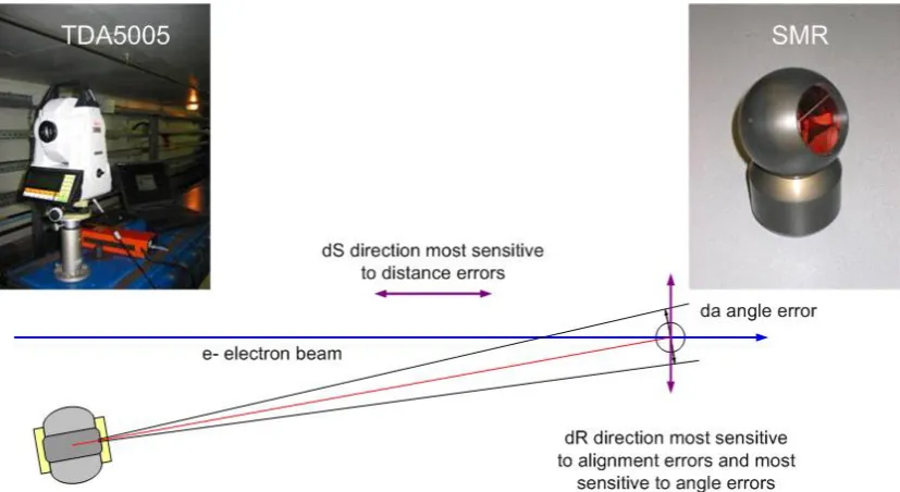
Figure 1.2 At the ESRF, as with most accelerators, the directions most sensitive to alignment

errors are those orthogonal to the direction of travel of the electron beam. Due to the constraints of the tunnel, the survey network is typically long and narrow. Under these conditions, the direction most sensitive to alignment errors is also the most sensitive to angle measurements... 5

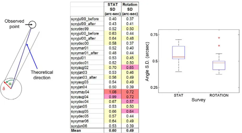
Figure 1.3 Angle residuals issued from 23 ESRF Booster Synchrotron (SY) network least

squares adjustment calculations. The angle residuals are given for STAT, and ROTATION. STAT represents the classical least squares calculation without the correction discussed in this

section. With the ROTATION results, the δ and αcorrection described above is applied to

the angle observations to optimise the angle residuals issued from the least squares

calculation... 6

Figure 1.4 The main objective of this thesis is to establish two traceable standards that can be

used to calibrate angles issued from RTSs and LTs. It is principally concerned with the HCC, the VCC and SMS instruments. This figure places these standards in the larger context of calibration and testing in general. ... 8

Figure 2.1 Set up used by the TPM for the calibration of theodolite horizontal circles. ... 28

Figure 3.1 Interaction between the user, the instrumentation, the work piece being measured

and the measurement environment. [43]... 33

Figure 3.2 Schematic drawing showing the principal components in RTSs and LTs as well as

a catalogue of the main errors associated with these instruments... 34

Figure 3.3 Schematic of the ESRF calibration bench. Zoom a) is the instrument station; zoom

b) the servo carriage with the instrument and interferometer reflectors and zoom c) the interferometer station. After the zero error has been determined the servo carriage is moved in 10 cm intervals from 2 m to 50 m to determine the instrument cyclic (bias) error. (Drawing prepared from Solid Works design drawings made by B. Perret)... 41

Figure 3.4 Typical Interferometer (IFM), Absolute Distance Meter (ADM) and EDM distance

error curves. Different curves are from different instruments. The IFM and ADM curves are from three different instrument manufacturers. The EDM curves are three instruments of the

same manufacturer and type. The expanded uncertainties (k=2) in these calibration curves

are 0.050 mm for the IFM and ADM curves and 0.165 mm for the EDM curves... 42

Figure 3.5 Schematic of the HCC assembly showing reference plateau e), the rotation table f)

and the LEC system a), b), c), and d)... 43

Figure 3.6 The photoelectric or image scanning principle used with the RON 905 angle

encoders is based on two scale gratings with equal grating periods; the circular scale is moved relative to the fixed scanning reticule. Parallel light is passed through the gratings, projecting light and dark surfaces onto a photoelectric detector. When the two gratings move relative to each other, the incident light is modulated. If the gaps are aligned, light passes through, while, if the lines of one grating coincide with the gaps of the other, no light passes through.

Photocells convert these variations in light intensity into nearly sinusoidal electrical signals.47

Figure 3.7 Four signals from the four read heads located at 90 degrees intervals around the

graduated disk is rotated, these read heads ‘see’ four sinusoidal signals 90 degrees out of phase. This is illustrated in the upper left hand box. The two signals on opposite sides of the circle (I I₀, ₁₈₀ and I₉₀,I₂₇₀) are subtracted from each other giving the two signals 90 degrees out of phase shown at the bottom of the figure. These two quadrature signals are used to determine the interpolated angle functionα_RONi. ...49

Figure 3.8 When the plateau is moved through an angleθ, its RON 905 encoder (d), and four

read heads, move with it through the same angle (right hand image). Recall that the encoder gratings (a) are in continuous rotation. ... 51

Figure 3.9 Under normal operation (i.e. continual rotation of the encoder gratings), the plateau

RON 905 (RON1 at top) and fixed RON 905 (RON2 at bottom) output one quadrature

(v₁=cosγand v₂=sinγ ) signal each. Each period of these signals corresponds to the passage

of one RON 905 encoder grating which is equivalent to 36 arc-seconds of rotation. These

signals are combined (ATAN2) to give an angle 1

(

)

1 2

tan

RONi v v

α ₌ − _{producing the classical}

saw tooth arctangent (i.e. −πto π ) function α_RON1and α_RON2. These signals are redressed by

unwrapping the phase (Unwrap) which gives a line whose slope is a function of the speed of rotation of the gratings. Because the two encoder grating disks are rigidly connected, the slopes of the two lines are parallel. Subtracting one line from the other leaves residual angle errors associated with the LEC and its two RON 905 encoders (at far right)... 53

Figure 3.10 When the plateau is moved, the attached RON 905 (RON1), as well as its read

heads, also move with it (refer to Figure 3.8). This will induce a change in velocity of the

RON1 read heads with respect to the static situation (Figure 3.9) ‘constant’ velocity (i.e. 20

degrees/second), and with respect to the still static RON2 read heads. This will lead to a

frequency modulation of the RON1 quadrature signals and to a change in slope of α_RON1while

the plateau is in motion. When the movement stops, the situation will return to normal shown

in Figure 3.9. However, there will be a net change in the separation distance between the two

lines associated with α_RON1and α_RON2 corresponding to the displacement angle. Although not

visible (at right), the residual angle errors associated with the LEC and its two RON 905 encoders will still be present... 54

Figure 3.11 RTS and LT horizontal angle calibration procedure: a) Observe the target and

record the RTS angle readingθ_RTSi′ . Record HCC LEC angle issued θ_HCCi′ ; b) rotate the HCC

through the angle θ_HCCwithout moving the RTS; c) Rotate the RTS through the nominal angle

RTS

θ

− without moving the HCC; and repeat the RTS and HCC observations and record the

RTS angle readingθ_{RTS i}′ _{( )+1} , record HCC LEC angle θ_{HCC i}′ _{( )+1} and compare the angle

differences. This procedure is repeated the desired number of times. ... 57

Figure 3.12 Schematic of the VCC assembly. ... 60

Figure 3.13 Graphs showing the dependence of the vertical angle uncertainty ( )U α′ for the LT

(left) and RTS (right) as a function ofd₀. Shorter d₀results in a larger vertical angle range at

the cost of a larger uncertainty. Recall the best manufacturer’s measurement uncertainties are 2.0 and 0.5 arc-seconds for the LT and the RTS respectively. ... 62

Figure 3.14 The top graph shows the ESRF DCB profile as a function of distance. It shows the

Figure 3.15 These graphs show the apparent error in the angle reading reduced to an offset distance as a function of distance along the ESRF DCB. Each of these curves represents the mean value of between 5 and 15 determinations of 474 points along the DCB with respect to

the mean profile shown in the top graph of Figure 3.14. The bottom graph shows the results of

this apparent error using a LT instrument... 65

Figure 3.16 Schematic diagram of the laboratory where horizontal and vertical angle

calibration is performed with the HCC and VCC. ... 66

Figure 3.17 Temperature evolution over 100 hours at 16 different positions on a grid at 2.2m

height in the laboratory. The left hand graph shows the temperatures with respect to the thermocouple located above the RTS position. The right hand graph shows box plots for the 16 thermocouples temperature over the 100 hour period. There is considerable spatial

variation but small temporal variation. ... 67

Figure 3.18 The influence of refraction on light travelling through the atmosphere. The actual

distance travelled s′will be longer than the true distance s between points. Similarly there

will be an angle error ε_Rdue to the angle of arrival of the light... 68

Figure 4.1 Heterodyne dual frequency laser interferometer. ... 74

Figure 4.2 Abbe and cosine errors in interferometry. ... 74

Figure 4.3 Autocollimation principle used in electronic autocollimators such as the

ELCOMAT 3000. ... 76

Figure 4.4 Capacitive probe circuit used at the ESRF. ... 79

Figure 4.5 Lock in amplifier ... 80

Figure 4.6 Capacitive probe calibration bench showing: a) the servo-controlled target; b) the

probe support and c) the high precision interferometer. ... 82

Figure 4.7 Example of a capacitive probe calibration curve... 82

Figure 4.8 Donaldson Reversal method is shown showing example probe readings mF

( )

θ

andmR

( )

θ ; the artefact form errorfe

( )

θ ; the spindle motions

( )

θ ; and the form and spindle

error developed over 360 degrees. ... 86

Figure 4.9 Estler face reversal. ... 87

Figure 4.10 Setup for the multi-probe method of motion/form error separation. Several probes

are arranged around the artefact at anglesϕ ϕ ϕ₁, ,_{2 3}". Probe no. 0 is aligned along the xaxis. The probes are stationary and make readings m₁

( )

θ ,m₂

( ) ( )

θ ,m₃ θ "while the artefact rotates about its z axis. ... 89

Figure 4.11 The transfer functions forA_k and B_k in equation (4.18) become undefined when

0

j j

α =β = . This occurs at values for harmonics j where j k= ±1. In this example the upper

graphs shows αand β and the lower graphs show ₁

(

_α2_+β2

)

_for

1 22.5

Figure 4.12 Flow chart algorithm for the determination of the value of kfor rational fraction values of ϕ₁and ϕ₂. The Matlab code used to establish this flow chart is given. ... 98

Figure 4.13 Characteristics of the simulated signal for the form error – spindle motion

separation harmonic studies used in later sections of this chapter. This specific example has probe angles ϕ₀=0, ϕ₁=17 121π and ϕ₂=15 27π ... 99

Figure 4.14 A resonance diagram permits the localisation and visualisation of combinations of

angles

(

0, ,ϕ ϕ_{1 2}

)

where α_k±1=β_k±1=0. The top left hand graph, shows the intersection of the

two lines gives angles ϕ₁and ϕ₂ for which k=20. The top right hand graph shows a partial

resonance diagram. One remarks the symmetry between the 4 quadrants. The bottom graph

shows the combinations of anglesϕ₁and ϕ₂ for which k m< and it is not possible to separate

the form error from the spindle motion using the multi-probe technique... 101

Figure 4.15 In all of these graphsk m> . The top left graph show probe separation angles

1

ϕ and ϕ₂ for which the standard deviation of the separated form error is between 12.5 and

250 times that of simulated input error. The top right hand graph shows and example of the difference between the simulated form error and the separated form error. Graph b) shows the same for angles where the separated form error is between 3 and 12.5 times that of simulated input error. Graph c) gives the same as a) for angles where the separated form error is below 3 times that of simulated input error. ... 102

Figure 4.16 The left hand graph shows distributions of kvalues as a function of din the

relationϕ=n dπ with respect to an arbitrary cut off harmonic m=180. The right hand graph

shows that even for values of k for which the error separation is possible, there remains

considerable variation and unexpectedly high errors inSD fe

(

_sep− fe_sim

)

... 104

Figure 4.17 Selection of residual plots for which values of k >

(

m=180

)

. The top graph

shows the separated form error with the residuals (i.e.

(

fe_sep− fe_sim

)

) shown in graph b). .. 105

Figure 4.18 Plots of the standard deviation of the simulated theoretical form error subtracted

from the actual separated error SD fe

(

_sep− fe_sim

)

for three constant angles of ϕ₁, and ϕ₂varied by 1 degree steps between 1 and 179 degrees... 106

Figure 4.19 Behaviour of the separation error in the vicinity of ϕ₁ and ϕ₂. These graphs

should be viewed in light of the residual error plots shown in Figure 4.17... 108

Figure 4.20 Graph a) shows an example of the intrinsic error saw tooth function. Graph b)

shows box plots of mean abs

(

(

fe_sep− fe_sim

)

)

for 50 simulations of underlying form error for

the 50 randomly selected sample

(

ϕ ϕ₁, ₂

)

probe separation angle pairs. The probe reading

errors are zero. The same set of 50 form errors are used for each of the 50 probe separation angle pairs. ... 111

Figure 4.21 Dependence of SD fe

(

_sep− fe_sim

)

on the probe separation angle (i.e. simulation

sample number) ϕ₁and ϕ₂ and the underlying form error. For comparison, graph a) uses the

same form errors as those used in graph b) of Figure 4.20. Graph b) uses a random selection of

Figure 5.1 Illustration of the _{Bias Variance trade off. The training sample may represent the} 2

measured data arbitrarily well. However, it may not be very representative of the underlying

process or of a new series of measured data. There is some optimal point where the _Bias 2

variance trade off will minimize the prediction error. This graph, reproduced by the author, comes from p.38 of [102]... 122

Figure 5.2 For different smoothing models for the data presented in Figure 5.16. From the top

to the bottom graphs there is progressively more smoothing in the model (i.e. p=0.9 to

p=0.00000001). This is also the passage from a high Bias2, low Variance to a low Bias2, high

Variance model. ... 123

Figure 5.3 This _{Bias Variance trade off is derived from data discussed in} 2 _{Bias Variance} 2

trade off and Figure 5.2 above. As the pvalue increases (i.e. more smoothing) from left to

right, the variance of the training and test samples decreases. However at p=0.0001, the

variance of the test set levels off and later begins to increase. The variance of the training data set decreases continuously as the model approaches an interpolating function... 124

Figure 5.4 The top graph shows real RON905 differences (α_RON1−α_RON2) over three full turns

(1080 degrees) of the LEC RV120CC. Note the sampling rate here is 50 Ksamples per second rather than the regular sampling rate of 500 Ksamples per second. Recall that 360 degrees of

phase angle is equivalent to 36 arc-seconds of rotation, thus peak to peak α_RON1−α_RON2is in

the order of 1 arc-second. The lower graph shows the spectral content of the LEC

1 2

RON RON

α −α signal in dB per arc second of equivalent frequency. Recall the nominal LEC

rotation speed in 20º per second. There are notable peaks at 36 arc-seconds and its harmonics 18, 9 etc… arc-seconds. ... 126

Figure 5.5 The top graph shows LEC data sampled over 6 gratings at 500 kSamples/s. The

LEC has a revolution speed of 20 degrees per second so one grating of 36 arc seconds has 250

samples (i.e. 0.01°×

(

500 kSample/sec

) (

20 /sec°

)

). A smooth Fourier series basis function

(order 20) is passed through the data. The bottom left hand graph shows residuals with respect to this curve and the bottom right hand graph is a normal probability plot of these residuals.

... 128

Figure 5.6 LEC data gathered over 850 revolutions. Each revolution consists of 180 mean

values of 50 kSamples. The top graph therefore has 153000 points. The bottom graph is a zoom over 50 LEC revolutions. We see the characteristic oscillation over one LEC revolution

shown in Figure 5.4. However we also see a clear amplitude modulation with a period in the

order of 25 LEC revolutions. ... 129

Figure 5.7 The top graph shows mean values of the LEC over one revolution for 850

revolutions. These two graphs give the impression the mean values follow a random walk process and are hence not deterministic. The bottom left hand graph shows the difference between successive mean LEC values. The bottom right hand graph shows a normal probability plot of these difference values. This graph shows a Gaussian distribution which supports a random walk hypothesis for the meaned LEC data. ... 130

Figure 5.8 Folding the signal shown in Figure 5.6 so that we look at each LEC rotation one

after another shows that the error curve appears to move to the right as a function of LEC revolution number or time. Superimposed on this rightward motion is a second oscillation. It is this second oscillation that appears as a modulation in Figure 5.6. ... 131

Figure 5.9 A spinning top precesses about the vertical axis z. The forceMgGof the top due to

momentum vector LG. The torque b) changes the direction of the angular momentum vector

d +

LG LG causing precession. However, the there are actually two components to the total

angular momentum LG+dLGand LG_prdue to the precession and the resultant vector LG_totaldoes not generally lie in the symmetry axis of the spinning top. The difference between the ideal situation and the actual situation results in an oscillation called nutation of the top back and forth about the precsssional circle c)... 132

Figure 5.10 Three cases describing the precessional motion of a spinning top or gyroscope.

The first case a) results when there is an initial angular velocity in the direction of the

precession. Case c) results when there is an initial angular velocity in the direction opposite to the direction of precession. The most common case, and indeed the case of the LEC b) results from initial conditions θ θ= ₁ and ψ= =0 θ... 133

Figure 5.11 The top graph a) shows the sample number index of the maximum value in a

given revolution in Figure 5.8 as a function of the revolution number. This provides an

indication of the rate of precession which is estimated to be 0.1506 precession degrees per LEC turn. Now recuperating the phase angle corresponding to the maximum value index

(once again from Figure 5.8) and plotting against LEC turn revolution provides graph in b).

This resembles (an inverted version) the cusp form of Figure 5.10. Plotting each cycle of b)

one on another and centring gives c). From these graphs we can estimate the nutation cycle to be 3.5 degrees (or ±1.75 degrees shown by the vertical lines in c) of precession cycle. This

cycle is confirmed by the best fit 2nd _{degree polynomial (solid line in c) and the magnitude of}

the nutation is estimated to be 2× ±

(

0.09

)

arc seconds. ... 135

Figure 5.12 Probe data for the radial form error spindle motion separation (top graph) and face

error spindle motion separation (2nd graph from top). This data represents three cycles of movements. The forward and reverse movements as well as the wait periods, which are flat and zero valued, can be clearly seen. The same data is shown as a function of angle for the radial probes (2nd graph from bottom) and face probes (bottom graph). The heavy line is the radial and face probe number 1... 138

Figure 5.13 Zoom on the data taken from probe number 1 (bottom graphs) of Figure 5.12 for

the radial and face form error spindle motion separation. The top graphs show data for three consecutive forward and reverse movements of radial probe 1 between 0 and 5 degrees (left), 125 and 131 degrees (middle), and 355 and 360 degrees (right). Data collected during the wait periods is shown by a large number of clumped points in the left and right hand graphs. The same is shown for the face error probe number 1 in the bottom three graphs. These graphs also highlight the irregularity in the sampling of the data set. ... 139

Figure 5.14 Box plots showing the statistics for the wait periods before the forward

movements at 0 degrees ( 1F "F4), where 4F is at the end of the test; and before the reverse

movements ( 1R "R3) at 360 degrees shown in Figure 5.13. The left hand graph shows

statistics for radial probe 1, while the right hand graph shows statistics for face probe 1... 140

Figure 5.15 Application of the linear closure correction for radial and face probe number 1.

These graphs are to be compared to those in Figure 5.13... 142

Figure 5.16 Example of the use of a smoothing spline to examine the evolution of the face

Figure 5.17 Zoom of the three sections→R1−F1, 2→R −F1and 3→R −F1of Figure 5.16 with respect to their mean values... 144

Figure 5.18 The final probe readings corrected for the non-linear evolution and the systematic

closure error. This graph is to be compared with the original non-corrected data in Figure 5.13

and the linear closure correction in Figure 5.15... 145

Figure 5.19 Final results of the radial FESM (graphs a and b) and face error wobble and

zmotion error separations (graphs c and d). ... 147

Figure 5.20 The small angle experimental setup. On the left hand side is a schematic while on

the right hand side are two photos. The cut A is along the bar at the position of capacitive probes number 1 and 2. The bar was moved in small displacements of up to ±150 arc seconds or ±365µm at the capacitive probe positions (i.e. ~0.5 m from the centre). Angle

displacements were also measured by the ELCOMAT 3000 to a 12 side polygon mirror.

Positions of the temperature sensors are denoted by T1"T4 in the drawing to the left. A fifth

temperature sensor which is not shown was installed in the LEC encasement... 149

Figure 5.21 Experimental conditions for the small angle tests. Graph a) shows the raw

temperature. Graph b) shows the filtered temperature evolution. The blue line (i.e. largest displacements) is the temperature on the continuously rotating shaft of the LEC. Graph c) shows the plateau position over the experiment. ... 150

Figure 5.22 Experimental results of the small angle tests. The top graph a) shows the

differences between measured angles for the ELCOMAT 3000 and the LEC (blue) and the capacitive probes and the LEC (green). The middle graphs show the temperature models for the capacitive probes and the ELCOMAT 3000 versus the LEC shaft temperature (graph b) of

Figure 5.21. The bottom graph shows the temperature modelled differences between angles

for the ELCOMAT 3000 and the LEC (blue) and the capacitive probes and the LEC (green). ... 151

Figure 5.23 Apparent error of the LEC as observed by the ELCOMAT 3000. The error bars

give the manufacturer’s uncertainty of 0.2 arc seconds... 155

Figure 5.24 ELCOMAT 3000 observations and construction of the apparent LEC error using a

6th _{degree Fourier series. Dashed magenta lines show the 95% prediction intervals for the}

Fourier curve. The model standard deviation is 0.11 arc-seconds... 157

Figure 5.25 The trilateration test setup is show in drawing a). Three interferometer stations

were setup at approximately 800 mm from the centre of the HCC plateau separated by roughly 120 degrees. Three reflectors were installed on a support which rotated about the HCC centre

of rotation. The reflector normal directions δ_ndo not change with the HCC rotation angle β_i,

however, the reflector opening angles α_{i n} vary as a function of the HCC plateau position

(drawing b). These opening angles varied by approximately ±13.6 degrees... 158

Figure 5.26 Distances measured from the three trilateration stations to their respective

reflectors mounted on the HCC as the plateau is rotated through 360 degrees. ... 159

Figure 5.27 Laser tracker HCC verification setup. ... 160

Figure 5.28 Leica LTD500 laser tracker LEC verification results using the experimental setup

shown in Figure 5.27. The residual standard deviation with respect to the modelled curve is

Figure 5.29 The apparent LEC harmonic 3 error seen in the calibration curve of a RTS (TDA5005)... 162

Figure 5.30 Summary of the 6th _{degree Fourier curves of the apparent LEC harmonic 3 error}

curve... 163

Figure 5.31 Measurements are made to determine the positions of the radial

(

R1 R5"

)

and

vertical

(

V1 V5"

)

capacitive probes in relation to the autocollimator- polygon mirror to

calculate the orientations of each of the systems with respect to one another. ... 165

Figure 5.32 Graph a) shows the comparison between HCC collimation error determined by the

ELCOMAT 3000 polygon mirror the same determined by the capacitive probe method Graph b) shows the comparison LTD laser tracker and capacitive probe methods for thee

determination of the collimation error. ... 168

Figure 6.1 Schematic diagram showing the interaction between the different bodies in the

accreditation chain. The main players at the national level are the national accreditation bodies (e.g. UKAS and COFRAC) and the national metrology institutes (e.g. NPL and LNE).

Through the MRA and a common statement between BIPM, OIML and ILAC, measurements made by different NMIs and accredited laboratories are recognized between different

signatories. ... 173

Figure 6.2 Measurement scheme of the VCC. ... 184

Figure 6.3 Measured VCC profile errors. In the vertical angle calibration configuration, the R

error is in the direction perpendicular to the observation (the xdirection in Figure 6.2) and the

Z error is in the direction of the observation (the ydirection in Figure 6.2)... 187 Figure 6.4 Schematic of the VCC cosine and carriage errors. ... 187

Figure 6.5 VCC Type B uncertainty U va

( )

′ as a function of vertical displacement and VCC

zero position. In the top graph the zero position is taken to be at the top of the VCC while with the bottom graph it is taken to be at the centre of the VCC. The asymmetry in the bottom (and top) graph is due to the direction of the tilts in the xzand yzplanes. ... 200

Figure 6.6 The results of ten calibrations each for a Leica TDA5005 RTS, a Leica AT901-MR

LT and API Tracker II+ LT. The xaxis is the instrument zenithal angle and the yaxis gives

the difference between the measured and modelled (equation (6.2)) vertical angle in arc seconds... 201

Figure 6.7 Capacitive probe calibration using the method discussed in section 4.1.4. The top

left hand graph a) shows the displacement measured by the interferometer as a function of the probe output in Volts. The top right hand graph b) shows the residuals with respect to a best fit line through graph a). In graph b), 10 independent calibrations were made on the same capacitive probe. Graph c) shows box plots of the residuals of the 10 calibrations with respect to a degree 5 polynomial. Finally, to demonstrate its the long term stability, results of a calibration made on the same probe two years previously are superimposed on the results shown in b)... 203

Figure 6.8 Calibration results of 15 capacitive probes used in the validation experiments of the

Figure 6.9 Graph a) shows the evolution of 6 capacitive probes over a 50 hour period starting on 12 October 2007. Graph b) shows the evolution of thermocouples installed adjacent to the

probes. Graph c) shows the clear correlation between the capacitive probe evolution dSand

the temperature evolutiondT. ... 205

Figure 6.10 Development of the capacitive probe uncertainty model. Graphs a) and b) are the

full probe and temperature data sets for one probe. Graphs c) and d) are examples of a 60 minute part of the two data sets. Graphs e) and f) show a normal probability plot and histogram for the probe data and graph g) shows the mean standard deviations for the six probes at 10 time intervals. ... 207

Figure 6.11 Final capacitive probe temporal uncertainty model. Graph a) shows the

distributions for the 5 probe data sets at each of the selected time periods t. The bottom graph

shows the standard deviations for 250000 samples from these data sets for each of the time periods considered. ... 209

Figure 6.12 Summary of the standard deviations of difference between the capacitive probe

and ELCOMAT 3000 angle measurements and the LEC angle measurements with and with out the temperature corrections model of Figure 5.22. ... 210

Figure 6.13 Final uncertainty model for the small angle LEC tests using the capacitive probes.

The overall standard deviation of the points with respect to the modelled curve is _{0.6 10×} −4_arc

seconds... 211

Figure 6.14 The effects of introducing error into the FESM process. On the top row, the

effects (from left to right) of the combined probe reading and separation angle ϕ_i errors,

probe errors alone and probe separation angle errors alone, on the separated form error from the 10 combinations of three probes in the radial separation. The second row gives the same results for the 5 combinations of 4 probes and the bottom row the results for the five probe

combination. The reference form error (top graph in Figure 5.19) resembles closely that of the

three right hand graphs... 216

Figure 6.15 These histograms show the PDFs of the residuals of the form errors issued from

the previous simulations with respect to the reference form error (i.e. the mean value of the

form errors – top graph of Figure 5.19). Histogram a) is the PDF for the combinations of three

probes differences; histogram b) the PDF for the combinations of four probes; histogram c) the five probe differences and histogram d) the combination of all combinations (i.e. the

amalgamation of 3, 4 and 5 probes). The red curves show a Student's t-distribution fit and the

black curves show a Normal distribution fit to the data. ... 219

Figure 6.16 Results of the vicinity studies on real HCC plateau probe separation data based on

the techniques developed in section 4.2.4. The top graphs are the equivalent of the vicinity

graphs of ϕ₁ and ϕ₂shown in Figure 4.19. However for the sake of space all 10 curves are

superposed on one another. This is done by subtracting the nominal values for ϕ₁ and ϕ₂. The

black horizontal lines in these graphs represent the standard deviation of the simulated probe reading errors used. The middle graph is a resume of these graphs showing the values for

(

sep sim

)

SD fe − fe at the nominal angles ϕ₁ and ϕ₂. In the bottom graph, the two largest values of SD fe

(

_sep− fe_sim

)

(i.e. index by 2 and 5 in the middle graph) are plotted in red while the two smallest values (1 and 7) are plotted in blue... 221

Figure 6.17 Vicinity graphs of real data once again. However, this time there are real resonant

effects with the fifth combination of angles 0 , ϕ₁=119.843 and ϕ₂=279.900. In this case

Figure 6.18 Temperature profile of the laboratory in which the HCC and VCC are installed. Spatial variations can reach ±0.9 Celsius, largely due to the air conditioning unit. ... 224

Figure 6.19 Overview of the horizontal angle calibration process. ... 225

Figure 6.20 Influence of collimation axis error on horizontal angle observations made with

SMS instruments (after figure 333 [15])... 227

Figure 6.21 Two independent calibration curves with two different shim positions. The

horizontal axis gives the TDA5005 horizontal angle position with respect to its zero position. The black solid line gives the combined collimation error while the blue points give the difference between the TDA5005 horizontal angle readings and the LEC reading... 228

Figure 6.22 The residual errors of the TDA5005 horizontal angle readings minus the LEC

readings minus the combined collimation error for the calibration example presented in Figure 6.21 above. These curves represent the final calibration corrections to be added to the nominal horizontal angle readings referenced to the instruments horizontal angle zero position. ... 229

Figure 6.23 Resume of the 13 calibration curves made for the Leica TDA5005 serial number

438679. The top graph shows the residuals of al 13 calibrations the TDA5005 horizontal angle readings while the bottom graph shows the mean values and curves for the mean values ± one standard deviation. ... 230

Figure 6.24 Schematic showing the different inputs to the GUM supplement number 1

approach to the uncertainty calculation. ... 234

Figure 6.25 These graphs show the convergence of the lower and upper endpoints of the 95%

coverage interval and the standard uncertainty for 1500 simulations following the GUM supplement number 1 framework. The top graphs a) show the results for simulations when error is introduced into the instrument readings while the bottom graph show the results when no error is introduced. This case (b) represents the uncertainty of the HCC in the calibration of horizontal angles. ... 236

Figure 6.26 Probability density functions for the calibration of a TDA5005 (a), an API

Tracker II+ laser tracker (b). The bottom graph c) shows the PDF for the HCC. ... 237

Figure 6.27 ESRF storage ring radial error surface as a function of distance meter and

horizontal angle measurement uncertainty. ... 239

Figure 6.28 Calibration model for the TDA5005 RTS used in the main survey at the ESRF.

The RMSE of the fit is 0.37 arc seconds. ... 240

Figure 6.29 Calibration model for the API TrackerII+ LT. The RMSE of the fit is 1.07 arc

seconds... 241

Figure 7.1 The percentage contribution of Type B uncertainty to the combined uncertainty in

List of Tables

Table 2.1 Example industrial angle measuring instruments and manufacturers claimed or

generally accepted best uncertainties... 17

Table 2.2 Expanded uncertainties (k=2) taken from the NMI laboratory web sites at the time

of writing (March 2008). All values represent the best possible uncertainties expressed in arc-seconds... 19

Table 3.1 Principle of measurement, uncertainty and operating ranges of EDMs, ADMs and

IFMs integrated into LTs and RTSs... 36

Table 5.1 Oscillations between probe readings at 0 and 360 degrees (i.e. the same nominal

positions) during the waiting periods before forward and reverse movements. ... 141

Table 5.2 Standard deviations of the elements of the radial form error – spindle motion

separation and the face error motion separation. All standard deviation values are given in µm. ... 147

Table 5.3 Overall standard deviations of the uncorrected and temperature corrected

differences between; the capacitive probes measuring to the 1 m long bar, and the ELCOMAT 3000; and the angles determined by the LEC. ... 152

Table 6.1 Summary of the different uncertainty contributions to the VCC functional model

given in equation (6.1) and Figure 6.2... 185

Table 6.2 Contributions to and summary of the VCC interferometer distance uncertainty... 185

Table 6.3 Summary of the RTS measured distance uncertainty and contributions to it. ... 188

Table 6.4 Summary of the LT measured distance uncertainty and contributions to it. ... 189

Table 6.5 Summary of the capacitive probe calibration uncertainty where the final probe

calibration uncertainty is the square root of the sum of squared contributing uncertainties.. 204

Table 6.6 The temporal uncertainty summary for the capacitive probe data... 208

Table 6.7 The uncertainty summary for the capacitive probe used with the HCC. The

reference time period used is 4 hours. This corresponds to the maximum time required for a typical calibration... 209

Table 6.8 Expected LEC uncertainty for typical calibration periods and angle resolutions.. 212

Table 6.9 Standard uncertainties in of the separation errors with respect to the different probe

combinations in the radial FESM. ... 217

Table 6.10 Parameters for the Normal (_N

(

_{μ σ,} 2

)

_{) and Student’s t distribution t}

(

_, 2

)

ν μ σ

(Matlab t Location-Scale distribution – see footnote 39 on page 2). ... 220

Table 6.11 Representative refraction corrections for IFM distances, horizontal and vertical

angles through representative lines of sight with in the laboratory. ... 224

Table 6.12 Summary of the different uncertainty contributions to a HCC horizontal angle

Acknowledgements

I would like to acknowledge all those people who have helped me throughout this long

process.

First I would like to thank Pierre Thiry and Bill Stirling for having given me the

opportunity and encouragement to pursue this work at the ESRF.

I would like to thank my colleagues in the ESRF Alignment and Geodesy group; Daniel

Schirr-Bonnans, Christophe Lefevre and Noel Levet. In particular, however, I would like to

acknowledge the hard work of Bruno Perret, Laurent Maleval and Gilles Gatta without whom

the realization this project would have been far more difficult than it was. Bruno‘s advice,

Solid Works drawings and fabrication of all manner of mechanical bits and pieces, and

Laurent’s breadth of knowledge in electronics and interfacing complex equipment have been

invaluable. Gilles understanding of the art of uncertainty analysis, Labview programming and

patient experiments leading to the arduous Type A evaluations has been tremendously

appreciated.

I would like to thank my supervisor Professor Derek Chetwynd for his advice and the time

he has taken in reading and proposing improvements and clarifications to this work. The long

distance working arrangement between Coventry and Grenoble has been a pleasant challenge

that has worked out very well indeed.

Finally I would like to thank my wife Marie-Christine, and three children, Thomas,

Matthew and Rachel for their love and patience. It has not always been easy over the past

Dedication

Declaration

I declare that this thesis is my own work except for the following help with specific equipment and techniques:

• Several Type A repeatability tests on the horizontal angle comparator and vertical

angle comparator shown in Figure 6.6 and Figure 6.23 were performed by Gilles Gatta (ESRF ALGE group).

Information derived from the published or unpublished work of others has been acknowledged

in the text and a list of references is given.

This thesis has not been submitted in any form for another degree or diploma at any university

or other institution of tertiary education.

……….. ………..

Abstract

The European Synchrotron Radiation Facility (ESRF) located in Grenoble, France is a joint facility supported and shared by 19 European countries. It operates the most powerful

synchrotron radiation source in Europe. Synchrotron radiation sources address many important questions in modern science and technology. They can be compared to “super microscopes”, revealing invaluable information in numerous fields of diverse research such as physics, medicine, biology, geophysics and archaeology.

For the ESRF accelerators and beam lines to work correctly, alignment is of critical

importance. Alignment tolerances are typically much less than one millimetre and often in the order of several micrometers over the 844 m ESRF storage ring circumference. To help maintain these tolerances, the ESRF has, and continues to develop calibration techniques for high precision spherical measurement system (SMS) instruments. SMSs are a family of instruments comprising automated total stations (theodolites equipped with distance meters), referred to here as robotic total stations (RTSs); and laser trackers (LTs).

The ESRF has a modern distance meter calibration bench (DCB) used for the calibration of SMS electronic distance meters. At the limit of distance meter precision, the only way to improve positional uncertainty in the ESRF alignment is to improve the angle measuring capacity of these instruments. To this end, the horizontal circle comparator (HCC) and the vertical circle comparator (VCC) have been developed. Specifically, the HCC and VCC are used to calibrate the horizontal and vertical circle readings of SMS instruments under their natural working conditions. Combined with the DCB, the HCC and VCC provide a full calibration suite for SMS instruments. This thesis presents their development, functionality and in depth uncertainty evaluation.

Several unique challenges are addressed in this work. The first is the development and characterization of the linked encoders configuration (LEC). This system, based on two continuously rotating angle encoders, is designed improve performance by eliminating residual encoder errors. The LEC can measure angle displacements with an estimated uncertainty of at least 0.044 arc seconds. Its uncertainty is presently limited by the

Acronyms and Abbreviations

There are many acronyms and abbreviations. Generally the abbreviation is defined the first

time it is met in the text.

Abbreviation Term

ADM Absolute Distance Meter ATR Automatic Target Recognition

ALGE ESRF ALignment and GEodesy group

BIPM Bureau International des Poids et Mesures CAT Computer Aided Theodolite systems CGPM Conférence Générale des Poids et Mesures CIPM Comité International des Poids et Mesures CMM Coordinate Measuring Machine

COFRAC COmité FRançais pour l'ACcréditation DCM Distance meter Calibration Bench EDM Electronic Distance Meter/Measurement ESRF European Synchrotron Radiation Facility FDA Functional Data Analysis

FESM Form Error – Spindle Motion error separation

GUM Guide to the expression of Uncertainty in Measurement

GUM1 Supplement number 1 to the GUM

HCC Horizontal Circle Comparator

HTM Homogeneous Transformation Matri(x)(ces) HLS Hydrostatic Levelling System

IFM Interferometric Distance Meter

ISO International Organization for Standardization JCGM Joint Committee for Guides in Metrology LEC Linked Encoders Configuration

LNE Laboratoire National d'Essais LT Laser Tracker

MTBF Mean Time Between Failure

NIST National Institute of Standards and Technology NMI National Metrology Institute

NPL National Physical Laboratory PDF Probability Density Function

PTB Physikalisch-Technische Bundesanstalt RMSE Root Mean Squared Error

RTS Robotic Total Station

SI International System of Units/Le Système International d'Unités

Abbreviation Term SR Storage Ring

UKAS United Kingdom Accreditation Service UPR Undulation Per Revolution

VCC Vertical Circle Comparator

VIM ISO/CEI GUIDE 99:2007: International Vocabulary of Metrology

1

Introduction: challenges in super-precise large scale

metrology

1.1

Introduction

This thesis addresses the problem of the calibration of spherical measurement systems

(SMSs). By SMSs we are referring to laser trackers (LT) and robotic total stations (RTS).

These instruments are used extensively in large scale (volume) metrology. They are able to

determine three dimensional coordinates of a point by measuring two orthogonal angles

(horizontal and vertical) and a distance to a reflector.

Large scale metrology includes fields that require very high precision alignment over

relatively large areas and volumes such as particle accelerator alignment, aircraft and vehicle

manufacture. The field of particle accelerator alignment for example is unique in that it overlaps both the fields of metrology and traditional surveying and geodesy. Standard

measurement precision is typically sub-millimetric over distances ranging between several

hundred metres and nearly 30 km! New and planned machines go beyond even this, requiring

micro-metre alignment precision on the same scales. The use of extremely specialised

techniques and instruments are needed to guarantee that these requirements can be met.

A review of some instruments used in, and examples of large scale metrology objects can

be found in [1]. A repository of papers presented during the regular International Workshop

on Accelerator Alignment (IWAA) can be found at [2]. This repository covers most fields

related to large scale metrology in accelerators.

In particular, a prerequisite to the attainment of these high degrees of precision is that there

confidence in the instruments employed and measurements made. One very important way in

which to assure this confidence is instrument calibration. Calibration is distinct from

instrument testing in so far as it establishes a relation between the measurand1 _{(e.g. distance or}

angle) with its measurement uncertainties provided by a measurement standard and the

corresponding indications with associated measurement uncertainties given by a measuring

instrument or system. Calibration is built upon the concept of traceability2_.

The problem of the calibration of the electronic distance meters (EDM) integrated into SMS

instruments has been studied extensively. However, at present there is neither a standard nor

even an instrument capable of calibrating the angles issued from these instruments under their

typical operating conditions and over their full measurement range (i.e. 360 degrees for the

horizontal vertical circles/encoders). This thesis proposes two instruments designed

specifically to investigate the angle measuring capacity of laser trackers (LTs) and robotic

total stations (RTSs). It then goes on to rigorously analyse their behaviour and provide a

detailed statement of their uncertainty.

This chapter will set the stage with a discussion of the background context to the

development of these instruments and a brief outline of the thesis.

1.2

Context summary

1.2.1

The European Synchrotron Radiation Facility

Many important questions in modern science and technology cannot be answered without a

profound knowledge of the intimate details of the structure of matter. To help in this quest,

scientists have developed ever more powerful instruments capable of resolving the structure of

matter down to the level of atoms and molecules. Synchrotron radiation sources, which can be

compared to “super microscopes”, reveal invaluable information in numerous fields of

research including physics, medicine, biology, meteorology, geophysics and archaeology to mention just a few. There are about 50 large research synchrotrons in the world, not to

mention smaller rings used in hospitals etc…, being used by an ever-growing number of

scientists and engineers.

The European Synchrotron Radiation Facility (ESRF) located in Grenoble, France is a joint

facility supported and shared by 18 European countries. It operates the most powerful

synchrotron radiation source in Europe. The annual budget for the operating costs of the

ESRF is of the order of 80 million Euros. Approximately 600 people work at the ESRF and

2 _{Property of a measurement result whereby the result can be related to a reference through a}

more than 6000 researchers come each year to the ESRF to carry out experiments. More than

1900 applications are received each year for beam time and about 1500 papers are published

annually on work carried out at the ESRF[3].

For the ESRF accelerators and beam lines to work correctly, alignment is of critical

importance. Alignment tolerances are typically less than one millimetre and often in the order

of several micrometers over the 844m Storage Ring (SR) circumference.

The ALignment and GEodesy (ALGE) group is responsible for the installation, control and

periodic realignment of the ESRF accelerators and experiments3_{. The uncertainty in distance}

and angle observations issued for the SR survey network calculations are in the order of 0.1

mm and 0.5 arc-seconds respectively. The uncertainty in the point determinations, as expressed by their absolute error ellipses, is less than 0.15 mm (semi-major axis) at the 95%

confidence level.

To help ensure these results, the ESRF has a 50 m long distance meter calibration bench

(DCB). This bench is used to calibrate the distance meters integrated into the robotic total

stations (RTSs) and laser trackers (LTs) used for all of the high precision metrological work at

the ESRF. Since February 2001, this bench has been accredited by Comité Français pour

l'Accréditation COFRAC (accreditation number 2-1508), under the ISO/CEI 17025 standard.

[4] COFRAC is the official French accreditation body. It is equivalent to and recognized by

the United Kingdom Accreditation Service (UKAS) in the UK.

At present, the limit to which calibration can be used to improve the distance measuring

capability of the instruments used to determine the ESRF survey network has been reached.

The only way to further better results is to improve the angle measuring capacity of these

instruments. The SMS angle calibration standards were developed to address this problem in

the context of alignment of the ESRF. Nevertheless, as with the ESRF DCB, the angle

standards can be applied to almost all types of LTs and RTSs available on the market.

3 _{Experiments are installed on beamlines. Typically there are several alignment critical components on}

1.2.2

Planimetric alignment at the ESRF

At the ESRF the main survey networks are measured with high precision RTSs equipped

with automatic target recognition (ATR). The instrument of choice (at the time of writing) is

the Leica TDA5005. This instrument measures both distance and angles. However, because of

[image:27.595.113.532.185.408.2]

the nature of the ESRF survey networks, angle measurements are of greatest importance.

Figure 1.1 The ESRF Storage Ring (SR) planimetric survey network.

The ESRF planimetric survey is based on a very regular network composed of 32 cells. In

each cell there are 3 instrument stations of which two are symmetric. Each instrument station

makes the same observations in each cell: stations 1 and 2 have 14 distance/angle observations

each and station 3 has 28 distance/angle observations. We remark that this is a long narrow

network (Figure 1.1) which is typical of most particle accelerators.

At the ESRF the direction most sensitive to alignment errors is orthogonal to the travel of

the beam. Because of the confines of the tunnel this direction is also the most sensitive to

angle measurements. This is illustrated in Figure 1.2. At present we are at the limit of distance

precision of the TDA5005. To improve the survey results, we must improve the angle

[image:28.595.118.532.61.287.2]

Figure 1.2 At the ESRF, as with most accelerators, the directions most sensitive to alignment errors are those orthogonal to the direction of travel of the electron beam. Due to the

constraints of the tunnel, the survey network is typically long and narrow. Under these conditions, the direction most sensitive to alignment errors is also the most sensitive to angle measurements.

To better understand the problem of the bias in angle error residuals, we will look at a study

made at the ESRF which helps to illustrate the influence of angle errors on the survey network

calculation (Figure 1.3). [5]

Consider that the centre of the horizontal angle reading system and the centre of rotation of

the instrument are not coincident but offset by a value δ . Choosing an angle α one can

correct all of the observed angles for an eccentricity with respect to the observation axis. One

can then minimise the standard deviation of the angle residuals issued from the least squares

calculation by iteratively varying the values of δ and α for each instrument used in the

survey and re-running the calculation to find the minimum of the angle residuals.

The angle residuals are given for STAT, and ROTATION. The STAT denomination

represents the classical least squares calculation without the δ and α corrections. The

ROTATION heading is used for the δ and α modified results. The results of this study

(Figure 1.3) shows convincingly in the right hand box plot labelled ROTATION, that even

though we cannot state their origin, we can affirm that with the classical least squares case the

angle residuals are not minimum. This result could imply that there are systematic angle errors

One of the principal aims of this project is to develop an angle calibration curve that can be

[image:29.595.116.521.110.332.2]

reliably used to help improve the results of the survey network calculations.

Figure 1.3 Angle residuals issued from 23 ESRF Booster Synchrotron (SY) network least squares adjustment calculations. The angle residuals are given for STAT, and ROTATION. STAT represents the classical least squares calculation without the correction discussed in this

section. With the ROTATION results, the δ and αcorrection described above is applied to

the angle observations to optimise the angle residuals issued from the least squares calculation.

1.3

The spherical measurement systems calibration program

The SMS calibration program is a suite of three instrument standards dedicated to the

calibration of the distance meters, and the horizontal and vertical circles of LTs and RTSs.

Traceability requirements, financial considerations and instrument constraints impose that

these three component parts be calibrated separately at the ESRF.

Electronic distance meters (EDMs), absolute distance meters (ADMs) and interferometric

distance meters (IFMs) are calibrated using the dedicated distance meter calibration bench

(DCB) that we have already introduced. The horizontal circles of RTSs and LTs are calibrated

using the horizontal circle comparator (HCC). The vertical circles are calibrated using the

vertical circle comparator (VCC). The majority of the present work is dedicated to the design,

calibration and error compensation of the HCC and to a lesser extent, the VCC.

The HCC is an instrument designed to provide an angle standard over the full 360 degree horizontal circle. Calibration is made by direct comparison of the spherical measurement