Estimation of a microfounded herding model on German survey expectations

(1)

WORKING PAPERS SERIES

WP07-07

(2)

Estimation of a Microfounded Herding Model

On German Survey Expectations

June 2007

Abstract

The paper considers the dynamic adjustments of an average opinion index that can be derived from a microfounded framework where the individual agents switch between two kinds of sentiment with certain transition probabilities. The index can thus represent a general business climate, i.e., expectations about the future course of the economy. This approach is empirically tested with the survey expectations published by the ZEW and ifo institute. The estimated co-efficients make economic sense and are highly significant. In particular, besides effects from fundamental data like the output gap in the recent past, one can identify a strong herding mechanism within both panels, such that metaphor-ically speaking the agents do not just join the crowd but follow each single motion of it. In addition, the transition probabilities of the ZEW agents are found to be influenced by the ifo climate but not the other way round.

JEL classification: D 84, E 32, E 37.

(3)

1 Introduction

While homogeneous rational expectations are still the ruling paradigm in macroeconomic

theory, expectations in the real world are far more diversified and may approximate rational

expectations, if at all, only in the aggregate. Being sufficiently self-critical, insecure, and

uncertain of the future events, the individual agents are eager to learn about the

expecta-tions of others, or about a general climate that is currently prevailing. This is the reason

why real-world agents, and financial markets in particular, closely monitor the periodic

publications of economic survey indicators.1

The evaluation of survey expectations is usually concerned with their ability to predict

the future course of the economy. Thus, in the case of Germany and the four surveys

available for this country, the ZEW and the ifo expectations indices are held to show the

best performance regarding economic growth (see, e.g., Broyer and Savry, 2002), where

the ZEW index could be praised to have the highest correlation with industrial production

when it is leading five to six months, vis-à-vis the ifo expectations with a lead of three or four months (Stadler, 2001; Hüfner and Schröder, 2002a,b). On the other hand, what is

lacking in these discussions is a conceptual framework that describes how an opinion index

may be formed and how it adjusts over time; with a particular view to possible herding

effects of the responding subjects where, for example, optimism feeds optimism. The topic

is of more than remote theoretical interest since a pronounced herding mechanism would

run counter the abovementioned rational expectations.

One step in the direction of a better understanding of the factors driving the survey

expectations is a study by Lahl and H¨ufner (2003) on the ZEW Indicator of Economic

Sentiment. Using ordinary least squares they find that besides a few lags of this variable

itself, each the German manufacturing order data, the German term structure, and the

US Consumer Confidence indicator have some additional explanatory power, too, a result

that is also confirmed by out-of-sample forecasts.2 _{The dynamic adjustments of the ZEW}

Indicator can thus be described as a combination of self-reference, as represented by the

1_{It may here also be noted that in contrast to macroeconomic theory which almost exclusively focusses}

on inflationary expectations, these surveys mainly relate to economic activity as a whole.

2_{Taking up the previous footnote, we find it remarkable that among the other independent variables}

(5)

significant autoregressive coefficients in the estimation, and of hetero-reference (Orl´ean, 1989). The latter expression means the state of opinion of a social group in its relationship

to an external norm, which is here given by a set of central macroeconomic variables in the

real, financial and foreign sector.

The investigation by Lahl and H¨ufner helps identify basic components in the

deter-mination of a survey index. Nevertheless, despite the motivation behind the selection of

the explanatory variables, the regression equation is not yet an economic theory. Although

it might be tempting to interpret the autoregressive coefficients as reflections of a herding

effect, the structure in the regression equation is too poor to warrant such a conclusion.

Alternatively, the coefficients may just as well result from some inertia in the adjustment

process, or the index itself may move quite in line with other economic variables that are

relevant to the survey participants.

This is where the present paper sets in. Reviving and slightly extending a more than

20-years old approach by Weidlich and Haag (1983), it provides a rigorous microfoundation

to explain the changes in a climate index such as the ZEW Indicator. For short, this

approach may be described as a herding dynamics. It easily captures the self-referential

and hetero-referential mechanisms, and it admits of a clearer specification of the, so far,

rather vague idea of herding. By virtue of its relatively parsimonious design, the model

can be directly estimated by nonlinear least-squares, which we will do for the ZEW as well

as for the similarly constructed ifo expectations index. The results may be of interest to

understand the dynamics of the two indices and to reveal the features that they share or in

which they differ. Our main concern, however, is an empirical validation of our approach to

model in a rigorous way such a psychologically contaminated concept as a general business

climate, which is akin to the famous ‘animal spirits’.

The remainder of the paper is organized as follows. Section 2 begins with a short

overview of the historical background of the model here put forward. It then introduces the

agents’ transition probabilities that govern their switches between two opposite attitudes,

derives an adjustment equation for the aggregated attitudes, i.e., for the general climate

index, and considers several feedback variables with which the transition probabilities may

vary. Section 3 tackles the nonlinear least-squares estimations of the basic model thus set

up. These results are contrasted with a straightforward linear regression approach, which

(6)

model. The imprecision problems are resolved at the end of Section 3. Section 4 contains

two parts. The first one examines whether the transition probabilities of the ZEW agents

are also influenced by the ifo climate index, and the other way round. In the second part

an additional variable is introduced which is unobservable and to some extent can capture

the effects that have so far been omitted. This generalization of the model is estimated by

the (extended) Kalman filter. Section 5 concludes.

2 The dynamic adjustment equation of the climate

index

2.1 Historical background

As indicated in the Introduction, the model we propose originates with a stimulating book

in the social sciences by Weidlich and Haag (1983). Unfortunately, their approach has not

found its way into contemporary macroeconomic theory, although for (heterodox)

econo-mists working with feedback-guided macrodynamic systems it would have been an

excep-tionally fruitful design. In our opinion, two reasons are responsible for this neglect. First,

the formulation of the model does not only refer to a probabilistic framework, its analysis

also uses concepts from the theory of statistical mechanics like the master equation and the

Fokker-Planck equation that are largely unknown to many economists. They are used to

study definite time paths of aggregate variables, whereas statistical mechanics is concerned

with the evolution of an entire probability distribution or at least, in the mean field

ap-proximations, with the time path of expected values. Even the latter concept, however, can

be hard to assess, namely, if the stochastic equilibrium of the system is characterized by

a bimodal probability density function, in which (otherwise most appealing) case expected

values would become meaningless in predicting the likely value of a variable.

A second aspect is insufficient marketing. While the approach was (also) employed

in a number of macroeconomic papers, the topics they dealt with were somewhat detached

or “exotic” (Kraft et al., 1986; Haag et al., 1987; Weise and Kraft, 1988), or the ordinary

reader probably soon drowned in a sea of specification details so that he or she could

no longer get hold of the attractive essence of the approach (Weidlich and Braun, 1992).

(7)

several related articles by, in particular, Kirman (1993), Lux (1995, 1997, 1998), or Orl´ean

(1995), all of which appeared in highly reputable journals that most of them will have

browsed on a regular basis. In sum, the approach by Weidlich and Haag (1983) or similar

formulations in the 1990ies offered macroeconomists a good chance to introduce herding

dynamics into their models in a very convenient, even standardized way, but this chance

was largely missed.3

Taking up the original specification by Weidlich and Haag, we content that for our

present purpose the whole statistical mechanics apparatus could be dispensed with.

In-stead, in that language, we can concentrate on a self-contained derivation of the Langevin

equation. Accordingly, an ordinary stochastic or deterministic, difference or differential

equation will emerge which can subsequently be analyzed, simulated, or estimated like any

other adjustment equation of this type.

2.2 From microscopic transition probabilities to a macroscopic

adjustment equation

Consider a fixed population of 2N agents where at time t each agent is either optimistic or pessimistic about the future prospects of the economy. Designating an optimistic and

pessimistic attitude by (+) and (₋), respectively, let n+_t , n−_t be the number of optimistic and pessimistic agents at t (n+t +n−t = 2N). Next, put nt = (n+t − n−t )/2 and define

xt = nt/N. All agents having equal weight in the population, this ratio is the average attitude of agents or, as we will call it, the climate index. Clearly, −1≤xt ≤1; optimism and pessimism balance in a state xt= 0; and at xt > 0 (xt < 0) optimistic (pessimistic) agents form a majority.

3_{Taylor and O’Connell (1985), Franke and Asada (1994), and Flaschel et al. (1997, Chapter 12) are}

(8)

Agents may change their attitude over time. We model this in discrete time and

slice time into adjustment periods of length ∆t > 0. That is, the agents’ attitudes are considered at time t, t+∆t, t+2∆t, etc. The individual changes will depend on a great variety of idiosyncratic circumstances, which one will not want to specify in all of their

details. It rather seems suitable to introduce random elements in this respect, in order to

keep the modelling simple and to avoid arbitrary assumptions. Therefore, the basic concept

to describe the changes in the climate index are the transition probabilities of the individual

agents: at time t, let π_t−+ be the probability per unit of time that an agent changes from pessimistic to optimistic, and π+t− the probability for an opposite change. More exactly,

∆tπ_t−+ is the probability that an agent who is pessimistic att has become optimistic at the next point in timet+∆t; and likewise∆tπt+− for an optimistic agent.4 These probabilities are uniform across the population. They are, however, not fixed but are influenced by the

variations of certain macro variables, which will be discussed further below.

Let us beforehand examine how, givenπt+− and π−t+, the climate index changes from

t to t+∆t.5 _{If we consider the ‘excess’ number of optimistic agents} _n_{t, it rises by 1 if a}

pessimistic agent becomes optimistic (when n+t increases andn−t decreases by 1). Symmet-rically, nt declines by 1 if an optimistic agent turns pessimistic. Denoting by kt+ and k−t the number of converts of the first and second type, respectively, we have

nt+∆t = nt + kt+ − kt− (1) As the number of pessimistic agents at timet can be written as n−_t =N ₋nt, the number

kt+ of agents turning optimistic can be viewed as arising from N−nt random draws each of which has probability∆tπt−+ for the event ‘+1’ (and the complement for the no-change event ‘0’). The number of these events are then added up. Hence, the random variable k+_t

has a binomial distributionB(N−nt,∆tπt−+). Analogously, n+t =N+ntbeing the number of optimistic agents in t, the random variable k_t− is distributed as B(N+nt,∆tπ+t−).6

4_{Which does not rule out that an agent switches several times within this adjustment period, although}

this might not appear very plausible for periods of moderate length∆t.

5_{The following argument draws on Alfarano and Lux (2005, Appendix A1 and A2).}

6_{A binomial distribution} _B₍_m,_π_{) is the probability distribution for the number of successes (}_k_{) in a}

sequence ofmindependent sucess/failure experiments, each of which yields success with probabilityπ. The

probability of getting exactlyksuccesses is given by!m_k"πk₍₁

−π)m−k_{, the mean is}_m_π_{, and the variance}

mπ(1₋π). To be clear, we have presupposed that the individual agents are autonomous, i.e., the realizations

(9)

The expected values of these variables areE(k+

t ) = (N−nt)∆tπt−+andE(kt−) = (N+

nt)∆tπ+−_{, their variances amount to Var(}_k+

t ) = (N−nt)∆tπ−t+(1−∆tπt−+) and Var(kt−) = (N+nt)∆tπ_t+−(1₋∆tπ+_t−). If the expected values are large enough (exceeding 5 or 10), the binomial distributions are (very) well approximated by the Gaussian distributions with

the same first and second moments. Taking for granted that the population is large andnt not too close to the boundaries ±N, we get

k_t+ = E(k+_t ) +

#

Var(kt+) ξt+ , kt− = E(k−t ) +

$

Var(kt−)ξt− (2)

whereξ_t+ andξ−_t are two independent random draws from the standard normal distribution

N(0,1) (with mean zero and variance equal to one). Furthermore, the difference between two normal distributions yields a normal distribution again. Its mean is the difference

between the two single means, its variance the sum of the two single variances. For the

random variablekt=k+t −k−t , we thus have with reference to the climate indexxt=nT/N,

E(kt) = ∆t·[(1−xt)π−t+−(1+xt)π+t−]·N and Var(kt) =∆t·[(1−xt)πt−+(1−∆tπ−t+) + (1+xt)πt+−(1−∆tπt+−)]·N. It remains to divide (1) and (2) by N and we obtain,

xt+∆t = xt + ∆t·[(1−xt)πt−+ − (1+xt)π+t−] + [(

√

∆t Dt/

√

N)] ξt

Dt := (1−xt)πt−+(1−∆tπ−t+) + (1+xt)π+t−(1−∆tπt+−) , ξt∼N(0,1) (3)

Equation (3) abstracts from the many individual and accidental switches in the agents’

atti-tudes and summarizes them in a macroscopic stochastic equation that governs the changes

in the climate index. It is the so-called Langevin equation that was announced above (here

specified in discrete time). The equation is usually derived by first setting up the entire

probability distributionP=P[x(t), t;z(·)] of x at timet, possibly given the time path of a set of exogenous variables z. To analyze ithe rate of change of P the powerful tool of the Fokker-Planck equation (FPE) is employed, which is itself a second-order approximation.

Regarding (3), the intimate connection between FPE and the Langevin equation is shown

by the fact that the first term in square brackets is the drift coefficient andDt corresponds to the fluctuation or diffusion term in FPE.7

other (which, depending on the specific social context and its network structure, might not be completely obvious).

7_{See Weidlich and Haag (1983, pp. 22 – 26) for a succinct presentation of the relationship between FPE}

(10)

On the other hand, if one is not interested in the distributionP and its evolution over time, the concept of FPE could be circumvented altogether and the story leading to eq. (3)

may fully suffice. In fact, the assumptions required for (3) to be valid are not essentially

stronger, at least for economists, than those underlying the derivation of FPE.

Three special cases to which the adjustment equation (3) gives rise are easily

recog-nized. First, the noise level decreases with the size of the population and in the limitN_→∞, the herding dynamics becomes a deterministic process (provided πt−+,πt+− do not, directly or indirectly, increase with N). Second, the continuous-time limit ∆t_→0 is well-defined, too. If (3) is written as xt+∆t = xt+A∆t+D%ξ

√

∆t, then this equation corresponds to the stochastic differential equation dx =A dt+D W% , where W is a normalized Brownian motion. Lastly, with A = A(x, z) in this equation, an infinitesimally short adjustment period ∆t, and an infinitely large population, the adjustments in (3) ‘degenerate’ to an ordinary differential equation ˙x = A(x, z).8 _{Note that especially the deterministic cases,}

taken on their own or when incorporated into a more comprehensive framework, could be

analyzed like any other difference or differential equation. These remarks show the wide

scope of eq. (3) for macrodynamic modelling. All will then hinge on the specification of the

transition probabilities, to which we now turn.

2.3 Feedbacks in the individual transition probabilities

Generally, the transition probabilities πt+− and πt−+ between t and t+∆t will change in response to the variations of a set of several variables that the agents observe. To ease

the exposition, let us summarize the variables in a single feedback index ft, which can attain positive and negative values in different stages the economy goes through. Positive

and negative are related to the probabilityπ_t−+ of switching from pessimistic to optimistic, that is, an increase in the feedback index increases πt−+ and decreases the complementary probability π+_t−.

It is an obvious concept, which Weidlich and Haag (1983) have also found very helpful

in their formal analysis, to assume that the changes of the transition probabilities depend

on the changes of the index ft in a linear way. More precisely, the relative changes, so

8_{More scrupulously, first}_N _{→ ∞}_{and then}_∆t_→_{0; or}_N _{tends faster to infinity than}_∆t_{to zero, such}

(11)

that we have dπ−+

t /πt−+ =αdft for some positive constant α. By suitably scaling f, this constant can be set equal to one. Symmetry is another natural assumption to make, which

gives usdπ_t+−/π_t+−=₋dft. Introducingν >0 as an ‘integration constant’, the specification of the transition probabilities reads (‘exp’ being the exponential function),

π−_t+ = π−+(ft) = ν exp(ft) , π+_t− = π+−(ft) = ν exp(₋ft) (4)

Certainly, (4) ensures positive values of the probabilities. The complementary condition

that the feedback index is bounded such that the probabilities are less than unity should

be a property of the model into which (4) is incorporated, or the outcome of an empirical

estimation.

A special feature of (4) is π−t+ = πt+− = ν > 0 when ft= 0. Hence even in the absence of active feedback forces or when the different feedback variables neutralize each

other, agents will still change their attitude with a positive probability. These reversals,

which can occur in either direction, are to be ascribed to idiosyncratic circumstances; they

appear as purely random from a macroscopic point of view and should cancel out in the

aggregate. For nonzero values of the feedback ft, the coefficient ν measures the general responsiveness of the transition probabilities to the arrival of new information. Soν can be generally characterized as a flexibility parameter(Weidlich and Haag, 1983, p. 41).

While eq. (4) provides a first and useful organizational device, the meaningfulness of

the model hinges essentially on the variables that are included in the feedback index. For a

basic specification, we concentrate on two variables which, we think, are the most

elemen-tary ones to consider. The empirical validity of the model is constituted by estimations in

the confines of this setting. Significant results are here also important if we want to sell

our approach as a building block ready for implementation in a more encompassing

macro-dynamic framework, where the user will appreciate a parsimonious specification. Although

adding further variables in the feedback index may be informative for specific purposes (two

such special issues will be examined later in Section 4), in general one will easily face the

problem of arbitrariness: what will be the reason for enriching the feedback index just by

this, but not another, variable?

The two variables whose influence on the transition probabilities we investigate are

(12)

from potential output (the precise definition is given below). We do not only consider the

levels of the two variables but, in order to capture possible accelerationist effects, also their

rates of change. In this respect, let us now fix the time unit as well as the adjustment period

as a month, ∆t = 1 [month]. Since the agents may guard against the noise that monthly variations can contain, changes over one or several months forxt andytare allowed to enter the feedback index, where the corresponding lags τx and τy may be distinct. Thus, in a formulation (and dating) that is directly suited for estimation, our model of the business

climate reads as follows:

xt = xt−1 + ν[(1−xt−1) exp(ft−1)−(1+xt−1) exp(−ft−1)] + εx,t (5)

ft−1 = φo+φxxt−1+φ∆x∆τxxt−1+φyyt−1+φ∆y∆τyyt−1 (6)

∆τuut := (ut−ut−τu)/τu for u=x, y (7)

Unlike the stochastic perturbations in eq. (3), the random terms εx,t are here assumed to have a constant standard deviation. Actually, the factor 1/√N in (3) will be typically so small that variations in the variance Dt can there be largely neglected. The present equation (5) rather conceives the εx,t as primarily representing random forces from outside our theoretical framework.

For conceptual reasons another source of randomness should be mentioned here, which

has its place still within the specification of the model. These are possible “measurement

errors”. In the first instance the term means that the agents, even if their information sets

were identical, do not observe the same data as those entering an estimation of (5) – (7). It

suffices to touch on the two most important discrepancies: (1) the period-(t−1) macro data may not have been available to the agents at that time or, if so, the data are likely to have

been revised by the statistical authorities in the meantime; (2) as will become clear below,

the agents had to determine the output gap in different ways from the econometrician.

It is therefore appropriate to include a second random influenceεf,t−1 in eq. (6), which

might also be serially correlated. Since, however, a corresponding amendment would require

a more elaborated estimation procedure, we postpone this device until later in Section 4.2.

For the time being, any such term εf,t−1 is omitted in (6) and we bear in mind that if

(13)

Accepting the limitation to two explanatory variables, the composition of the feedback

index is straightforward. Note first that the output gapy as well as its rates of change ∆y

are centered around zero. This allows us to interpretφo as apredisposition parameter, since in a neutral state where xt−1 = ∆τxt−1 = yt−1 = ∆τyt−1 = 0, a positive φo gives rise to a probability π−_t+ of switching from pessimistic to optimistic that exceeds ν =ν _·exp(0), while the reverse probabilityπt+− is less than ν.9

Referring to the expressions that were already mentioned in the Introduction, the

feedback of the climate index on itself can be said to represent the notion of self-reference

or, in more flowery language, herding, while the impact of the output gap on the climate

index is a hetero-referential mechanism. Regarding the herding aspect in the model, we

would like to underline that including xt−1 and ∆τxt−1 in eqs (5), (6) admits an explicit

structural interpretation with an immediate psychological plausibility, in contrast to the

more technical autoregressive coefficients in the estimation approach to the climate changes

by Lahl and H¨ufner (2003).10 _{Nevertheless, the natural presumption that optimism and}

pessimism are self-reinforcing, which would be reflected by positive coefficients φx or/and

φ∆x, will still have to be verified by the empirical estimations.

In finer detail, specification (6) distinguishes two variants of herding. A positive

coefficientφx means that the probability of switching from pessimism to optimism is higher, and the reverse probability of switching from optimism to pessimism is lower, the more

agents have already converted to an optimistic attitude. The herding effect expressed by

φx > 0 may thus be characterized as a majority effect. Moreover, on the basis of the arguments given in Appendix 1 the herding effect can be called weak if 0 < φx < 1, and strong if φx >1 is prevailing.

This notwithstanding, even a strong majority xt−1 may lose its attractiveness if it is

already crumbling off. This idea is captured by a positive coefficientφ∆x, which enables the

9_{Weidlich and Haag (1983, p. 41) call their counterpart of} _φ

o a preference parameter. Incidentally, a predisposition of the agents towards optimism does not necessarily imply that optimism dominates pes-simism in a stationary state of the adjustment equation (5) (underyt−1 =∆τyt−1= 0). In fact, this will depend on the coefficientφx: a stationary pointx"_{= 0 of (5) for}_φ

o= 0 is shifted upward by a risingφoif 0<φx<1, and thisx" shifts downward ifφx>1; see Weidlich and Haag (1983, pp. 42–44) and eq. (13) further below.

10_{The authors do not discuss the sign of their autoregressive coe}_ffi_{cients, let alone a possible conceptual}

(14)

negative change∆τxxt−1 in this situation to have a negative impact on the feedback index

ft−1 in (6). Generally, φ∆x > 0 assesses the effect that the probability of switching from pessimism to optimism is high (low) if in the recent past the number of optimistic agents

has increased (decreased), from what overall level of optimism or pessimism so ever. In

other words, the agents are keeping track of any changes in the current mood of the other

agents and (more or less unconsciously) adjust their transition probabilities accordingly.

Thus they view the motions of the crowd as an early warning system of future changes;

they do not discard these motions as temporary but (in terms of probabilities) respond

to them instantaneously. We actually consider this to be herding proper: an individual

sheep, to strain the metaphor and neglect the probabilistic setting, does not wait until the

great majority of the flock gathers at a greener grass and then joins them, it rather follows

the other sheep as soon as they begin moving. A markedly positive coefficient φ∆x can correspondingly be taken as another manifestation of strong herding, in the sense that it

captures the influence of the movements (not position) of the flock. In order to distinguish

this effect from high values of the level coefficient φx, i.e. from the majority effect, and still having the image of sheep in mind, it may also be said that the coefficient φ∆x > 0 measures a moving-flock effect.11

Turning to the second feedback variable in eq. (6), the basic ideas behind the effects of

the output gapyt−1or its rate of change∆τyyt−1on the business climate are now obvious. Of

course, the choice of this economic variable as a possible feedback need not be exclusive (as

exemplified by Lahl and H¨ufner, 2003, who try several other variables in their framework).

One should, however, start with a general activity variable, in level or growth rate form or

both. First because many other variables of interest may be closely correlated withyt−1 or ∆τyyt−1; and second because this raises the following question: are the agents really able

to predict the future course of these variables, or are the predictions rather determined by

the recent past of economic activity and its changes? Or is this no contradiction at all?

11_{The expression is not meant to carry a connotation of foolishness. At least for certain breeds of sheep}

(15)

In contrast to φx and φ∆x, the signs of the two coefficientsφy and φ∆y related to the output gap area prioriambiguous. On the one hand, high levels of output or above-average growth rates may reassure optimistic agents that their current optimism is justified, and

convince pessimistic agents that their fears have become obsolete. In this view, φy ≥ 0,

φ∆y ≥ 0. On the other hand, such a situation might also be interpreted as carrying the seeds of a future slowdown or even downturn. For example, the central bank could be

expected to raise interest rates, unless it has already done so. These fears of diminishing

business prospects would be reflected by negative coefficientsφy or/andφ∆y. It is thus an open and interesting problem whether the two coefficients would come out significant in an

empirical estimation, and if so, how they are signed.

3 Estimation of the climate index

3.1 The empirical data

As mentioned in the Introduction there are two leading sentiment indicators for the German

economy. These surveys, which are regularly published on a monthly basis, are carried out

by the ifo institute and the ZEW institute.12 _{While the institutes ask a series of questions}

and construct several indices, we focus on the respondents’ expectations of the general

business situation six months ahead.13 _{This horizon is the same for both institutes, and}

both of them categorize the answers into the options ‘better’, ‘worse’ or ‘just about the

same’, of which they report the difference between the percentages of ‘better’ and ‘worse’

answers. The index is thus in relatively good concordance with our specification of the

climate variable x in Section 2.2.

The main difference between the two surveys are the number of participants and

the economic sectors from which they are recruited. The ifo institute asks more than

7,000 business leaders and senior managers from all sectors except the financial sector (the

answers are weighted according to the importance of the single industries). In contrast, the

12_See_{http://www.ifo.de}_and_{http://www.zew.de}_{. In German, the ‘ifo’ institute usually presents itself}

in lower-case characters.

13_{Especially regarding the ifo institute, this index should not be confused with the climate or sentiment}

(16)

ZEW survey echoes the opinion of the German financial sector, i.e., the participants are

financial analysts and institutional investors from banks (comprising 77% of the sample),

insurance companies, and large industrial corporations. The number of subjects contacted

is about 350.

The ZEW survey has started later than the ifo survey, in December 1991. The data

we are using end with 2006:6. To get a first impression of the two expectation indices, the

series are plotted together in the top panel of Figure 1, where they are rescaled in order

to fit into the interval between ₋1 and +1. For a better comparison of the results and to be sufficiently bounded away from these end-points (cf. the derivation of eq. (2)), the

factor by which the original series are multiplied is tuned such that the two indices are

contained within an interval _±0.80. The ifo index attains a corresponding minimum in 1992:11 (plotted at t = 1992.83), the ZEW index a maximum in 2000:1.14

At a first glance, the two indices exhibit a similar and clearly cyclical pattern, possibly

with a tendency for the ZEW index to be slightly leading in the turning points. An obvious

difference are the levels of the two series, where from the second half of 1992 onward

the ifo index runs persistently below the ZEW index; the mean values are ₋0.135 and 0.329, respectively. From this descriptive point of view the ifo index can be characterized

as basically pessimistic, the ZEW index as optimistic. For our structural model it may

be expected that this difference finds expression in negative and positive predisposition

parameters φo.

The lower two panels of Figure 1 show the behaviour of the variable that is to represent

the model’s component of hetero-reference. As indicated in Section 2, we choose output for

this purpose. Specifically, we work with industrial production, since it is the only output

category available as monthly data and was also used in other work (H¨ufner and Schr¨oder,

2002a,b; see, in addition, the discussion in Broyer and Savry, 2002). For an export-oriented

country like Germany with its weak and passive domestic demand, the manufacturing sector

can, however, still be regarded as providing the basic impulses for the rest of the economy,

especially for the large subsector of the business-related services (Franke and Kalmbach,

2005). Manufacturing output therefore contains more information about economic activity

as a whole than its share of about one-third in the national product might suggest.

14_{Here and in the following it will be understood that when we refer to the ‘ifo index’ or ‘ZEW index’,}

(17)

[image:17.612.105.497.54.377.2]

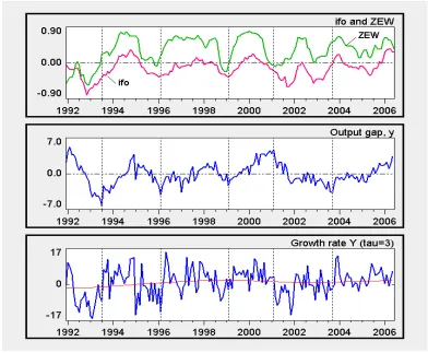
Figure 1: Time series of the data.

Note: The numbers in the second and third panel are percentages. The output variableY there is monthly industrial production. Detrending of log output uses the Hodrick-Prescott filter with smoothing parameterλ= 120,000; the growth rates are annualized 3-month changes. The thin line in the bottom panel is the trend growth rate implied by the filter.

The middle panel displays the output gap yt for this variable. It is defined as the percentage deviations of output from trend. The trend line is obtained by applying the

flexible Hodrick-Prescott filter to log output, with a smoothing parameter λ = 120,000. The reason for employing a roughly 8 times higher value than the conventional value of

14,400 is the variability in the implied trend growth rate (i.e., the slope of trend log output).

As can be seen from the thin line in the bottom panel, trend growth still exhibits sizeable

movements (though this is optically downplayed by the large fluctuations of the main series

in that panel): rising from −1.6% in 1992 to 1.9% in 1998, falling to 0.9% in 2002 and increasing again to 1.8% at the end of the sample. While one might wonder whether these

(18)

severe for the usual λ = 14,400. Nevertheless, since the deviations of the two- or three-month output growth rates from the trend rates are fairly large, and these deviations will

constitute the variable ∆τyyt:= (yt−yt−τy)/τy from eq. (7) in our estimations below, we

can do without a stronger smoothing of the trend and maintain λ = 120,000. The bold series in the bottom panel is in fact the annualized three-month growth rate of output.

A visual inspection of the comovements of the output gap with the two expectation

indices shows a (near-) coincidence of the troughs of yt and the ifo index in 1996:2 and 1999:2, slightly leaded by the ZEW index (see the vertical dashed lines in Figure 1). At the

two other troughs of yt in 1993:7 and 2003:9, however, both indices are already rising for more than six months (at least). Conversely, at the output peak in 2001:2 the indices are

on the downturn, the ZEW index being even just about to reach its next trough. Hence

there is no obvious pattern of synchronized movements, contemporaneously or lagged, of

the output gap and the expectation indices.15

In discussions of the indices it is rather more usual to compare them to the growth

rates of output. Regarding the 12-month growth rates (gt) of industrial production over the sample period 1992:1 – 2002:3, H¨ufner and Schr¨oder (2002a) report a significant lead ofθ= 2 months for the ifo index andθ= 5 months for the ZEW index, which they infer from the max-imal cross-correlation coefficients Corr(gt, xt−θ) = 0.88 and 0.81, respectively.16 Adding the

last four years to these observations and computing the cross-correlations Corr(∆12yt, xt−θ)

over our period 1991:12 – 2006:6, the first part of Table 1 largely confirms these results,

though the coherence is weaker and the leads are one month shorter (the bold figures in

the table indicate maximal coefficients). It is in this sense that the institutes praise the

predictive power of their indices.

It should be emphasized at this point that although lagged values ofxtare correlated with current growth rates of output or the output gap, for that matter, this does by no

means rule out that lagged output growth rates may also determine current expectations.

One reason is that in our equation (5) xt is determined jointly by several variables, the

15_{Statistically there are nevertheless cross-correlations Corr(}_y

t, xt−θ) = 0.47 atθ=6 for the ZEW index

and Corr(yt, xt−θ) = 0.60 atθ=5 for the ifo index, though this has not been sold as forecasting evidence so

far. In fact, given the relatively smooth character of the series, the coefficients should be somewhat higher than that.

(19)

Lead θ

4 3 2 1 0 ₋1 ₋2

∆12yt

ifo: 0.65 0.70 0.71 0.71 0.68 0.65 0.61

ZEW: 0.70 0.69 0.56 0.50 0.43 0.37 0.31

∆3yt

ifo: 0.17 0.26 0.34 0.41 0.45 0.49 0.48

[image:19.612.152.457.67.248.2]

ZEW: 0.34 0.38 0.37 0.39 0.41 0.42 0.41

Table 1: Cross-correlations of index xt−θ with growth rates

of monthly industrial production.

other reason that there, more precisely, lagged output growth does not act on the levels xt but on the first differencesxt−xt−1 of the expectation index.

In addition, the second part of Table 1 demonstrates that the forecasting capabilities

of the indices vanish if we refer to quarterly changes of output. Here, if anything, it is the

recent changes ∆3yt−1 that determine current expectations xt, rather than xt−θ predicting

∆3yt. In any case, whether lagged levels or growth rates of output can explain current

expectations, though jointly with a self-reference mechanism of the latter, must be an issue

of specific estimations.

3.2 Estimation of a semi-structural model

Before estimating the nonlinear modelling equations (5) – (7), it is useful to study a linear

regression approach that includes the same set of explanatory variables. In its general form,

we have the following ordinary least squares (OLS) estimation problem,17

xt = βo +

&

θ≥1

βθxt−θ +

&

θ≥1

γθyt−θ + εt (8)

17_{Regarding the scaling of the output gap in the estimation equations, a percentage deviation of, for}

(20)

The first month of the sample period underlying (8), which is the same for both the ZEW

and ifo expectations, is t = 1992:3, the last month is t = 2006:6. This amounts to a total of 172 observations.

Equation (8) has a minimal interpretation, in that it excludes any hypothesis of

rational expectations (no forward-looking variable on the right-hand side) and states that

the climate is determined by distributed lags just of itself and the output gap, and no other

variables. Beyond this, no further economic structure is made explicit. Linearity is then

the most convenient, if not only meaningful, assumption to make. The equation can be

thought of as being compatible with one or several (possibly linearized) model formulations

of business climate adjustments, which may already, or may not yet, exist. From this point

of view, the formulation in (8) is best characterized as a semi-structural model. On the

other hand, (8) can be given a specific interpretation if it is regarded as a linearization of

our adjustment equation (5) (eq. (10) below will provide the details).

The regressions in (8) are treated in several stages. The first stage is given by the

benchmark of a random walk process, according to which all coefficients are zero except

β1, which is fixed at unity. Beginning with the ZEW index, the resulting root mean square

error (RMSE) is reported in the first row of Table 2.

The second statistic in the table is two times the value L of the log-likelihood of the residuals εt (see, e.g., Davidson and MacKinnon, 2004, p. 403). Applying the likelihood ratio (LR) test (ibid., pp. 420f), this value will help us decide whether an estimation B with

rB independent variables is significantly better than a previous estimation A withrA < rB variables. The criterion is the difference (in obvious notation) LR = 2 [L(B)−L(A)], which for a large enough sample is approximately distributed as chi-square with r = rB −rA degrees of freedom. As can be read from any formulary, estimation B is significantly better

for r= 1 and r= 2 at a 95% level if LR > χ2

0.95(1) = 3.84, or if LR > χ20.95(2) = 5.99,

respectively.18

With this yardstick at hand, it can be checked step by step if additional regressors

yield a significant improvement. Compared to the random walk, there is no doubt about

18_{While the comparison of two log-likelihoods provides us with a statistical decision criterion, the root}

(21)

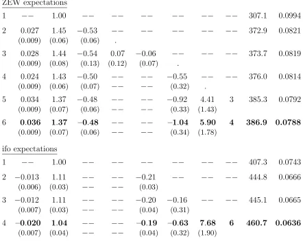
βo β1 β2 β3 β4 γy γ∆y τy 2 L RMSE ZEW expectations

1 −− 1.00 −− −− −− −− −− −− 307.1 0.0994

2 0.027 1.45 −0.53 −− −− −− −− −− 372.9 0.0821

(0.009) (0.06) (0.06) .

3 0.028 1.44 −0.54 0.07 −0.06 −− −− −− 373.7 0.0819

(0.009) (0.08) (0.13) (0.12) (0.07) .

4 0.024 1.43 ₋0.50 ₋₋ ₋₋ ₋0.55 ₋₋ ₋₋ 376.0 0.0814

(0.009) (0.06) (0.07) ₋₋ ₋₋ (0.32) .

5 0.034 1.37 ₋0.48 ₋₋ ₋₋ ₋0.92 4.41 3 385.3 0.0792

(0.009) (0.07) (0.06) −− −− (0.33) (1.43)

6 0.036 1.37 –0.48 −− −− –1.04 5.90 4 386.9 0.0788

(0.009) (0.07) (0.06) −− −− (0.34) (1.78)

ifo expectations

1 −− 1.00 −− −− −− −− −− −− 407.3 0.0743

2 ₋0.013 1.11 ₋₋ ₋₋ ₋0.21 ₋₋ ₋₋ ₋₋ 444.8 0.0666

(0.006) (0.03) −− −− (0.03)

3 −0.012 1.11 −− −− −0.20 −0.16 −− −− 445.1 0.0665

(0.007) (0.03) ₋₋ ₋₋ (0.04) (0.31)

4 –0.020 1.04 ₋₋ ₋₋ –0.19 –0.63 7.68 6 460.7 0.0636

[image:21.612.82.524.83.435.2]

(0.007) (0.04) ₋₋ ₋₋ (0.04) (0.32) (1.90)

Table 2: OLS estimations of regression (9).

Note: Numbers in parentheses are the standard errors, RMSE is the root mean square error of the predictions from the right-hand side of (9). 2 L is 2 times the value of the log-likelihood function. Thus, an estimation in a row with one (two) additional independent variable(s) is significantly better at a 95% level than that in another row if the difference exceeds 3.84 (or 5.99, respectively).

including a constant and the first two lags of the ZEW index; see the second row of Table

2. From this estimation on, (first-order) autocorrelation in the residuals is negligible, so no

Durbin-Watson or a similar statistic is reported.

Actually, we start out from a regression of xt on a constant and xt−1. The two

coefficientsβoandβ1 are both highly significant. Then we consecutively add one further lag

(22)

Complementarily, we add a large number of lags simultaneously and choose the lag with

the most significant coefficient. The result is in both cases the same, namely, lag θ = 2.

On this basis, with a constant and xt−1, xt−2 as regressors, we proceed in a likewise

manner to see whether another lag of xt can improve upon this estimation. Remarkably, this is not possible. The third row in Table 2 exemplifies this for adding lagsθ = 3,4, and the results are quite similar for other combinations of lags (up to θ= 13).

We note that the significance of only two lags of xt in eq. (8) is a good support for the specification of auto-reference in the feedback index of eq. (6), which is equally limited

to two lags of the climate. In fact, a sum β1xt−1 +β1+τxt−1−τ in (8) can be equivalently

written as (β1+β1+τ)xt−1−τ β1+τ∆τxt−1 if a rate of change is invoked (∆τxt−1 as defined

in (7)).

As far as the self-reference in (8) is concerned, we therefore settle down on a constant

and the two lagsxt−1,xt−2. Then, similar as above, we check whether, and with which lags,

the output gap can enhance the regression. The fourth row in Table 2 shows that including

the output gap yt−1 misses the LR criterion (376.0−372.9 = 3.1 < χ20.95(1) = 3.84; γy in the head of the table corresponds to γ1 in (8)). However, if we here do not stop short

but still add another, suitable lag, we find that it comes out significant and that now yt−1

is significant, too (it is discussed in a moment how this result shows up in Table 2). The

greatest gain in this respect is achieved with lag θ = 5. Moreover, all additional lags of the output gap (including its contemporaneous value withxt) lead to no further significant improvement.

Hence, also the specification of hetero-reference in our model’s feedback equation (6),

with one lagged level and one rate of change (as oft−1) of the output gap, is well supported by the investigation of regression (8). For a slightly more convenient presentation of the

two-lag significance results and other estimations in Table 2, we formulate eq. (8) as

xt = βo +

4

&

θ=1

βθxt−θ + γyyt−1 + γ∆y∆τyyt−1 + εt (9)

The sixth row of Table 2 presents the optimal fit that, as just mentioned, is achieved with

(23)

either. At least part of the lower coefficient on ∆τyyt−1 can be explained by the fact that

these changes are larger for the quarterly lag than for τy = 4.

The second part of Table 2 documents the central results from carrying out the same

battery of estimations for the ifo index. Generally, this series admits a better fit than the

ZEW index, as can be seen from its lower RMSEs and higher values of the log-likelihood.

It bears emphasizing that for both self- and hetero-reference, again only two lags prove to

be significant. With this additional support, the specification of the feedback equation (6)

can be claimed to be built on firm ground. The only difference between the ifo and ZEW

expectations are the lags involved: θ= 4 versusθ= 2 in the self-reference mechanism (which corresponds to τx= 3 versus τx= 1), and τy= 6 versus τy= 4 regarding the influence of the output rates of change.

3.3 First estimations of the structural model

After the investigation of the semi-structural adjustment equation of the climate index,

we can now return to the original model (5) – (7). Plugging (6), (7) into (5), we have a

regression that can be directly estimated by nonlinear least-squares (NLS).19_{Concentrating}

on the optimal lags of the explanatory variables from Table 2, the outcome is summarized

in Table 3.20

Let us again begin with the ZEW expectations. The first row corresponds to the

second row in Table 2 and presents an estimation where the model is confined to its herding

component. Besides the expected positive predisposition parameter, φo >0, both herding coefficients φx and φ∆x have the correct positive sign. However, the significantly larger likelihood statistic in the second row (2L = 385.2) makes it clear that, as before, these

19_{In an alternative attempt, Lux (2007) goes back to the micro level, sets up the abovementioned}

Fokker-Planck equation in (essentially) continuous time and computes from there the conditional transitional probability densities between two months, which can then be used for a maximum likelihood estimation. This approach is potentially superior since it seeks to exploit more information, though this goes at the price of a high computational effort and also its conceptual basis might slightly differ in detail. As yet, however, the relationship between the straightforward NLS approach of (5) – (7) and this more ambitious approach are not sufficiently well explored.

20_{We have checked that the optimality of these lags is indeed maintained in the estimation of the structural}

(24)

effects should be complemented by the feedbacks from the output gap. That is, the herding

mechanism has to be augmented by a mechanism of hetero-reference.

If the resulting likelihood is compared to the corresponding 2L = 386.9 in the sixth row of Table 2, it seems that the linear regression performs somewhat better, though it

is not significantly superior (the issue of the number of coefficients will be discussed in a

moment). It can thus be stated that, at least as far as the goodness-of-fit is concerned,

the structural model (5) – (7) is supported by the data. In addition, it will later be shown

that the fit can be substantially improved if the role of the random perturbations is slightly

modified.

It may also be observed that in contrast to the growth rate coefficientφ∆y, the coef-ficient φy on the level of the output gap is negative. According to the interpretation at the end of Section 2, the negative sign expresses certain doubts of the agents that a prosperous

phase of the economy will be sustained; or their hopes in a slump that the economy will be

able to recover.

Even if these results make good economic sense, the standard errors in parentheses

in the second row of Table 3 indicate that a great deficiency still remains, namely, the

imprecision of the estimates. If we follow the usual econometric standards then none of

the six coefficients is significantly different from zero. This is especially annoying for the

flexibility parameterν, since ν = 0 would be completely meaningless.

The imprecision of the coefficients may not come unexpectedly if the structural

equa-tions (5) – (7) are compared to the linear regression equation (9). The two approaches

differ on two counts: the structural model is nonlinear; and it contains one parameter “too

many”, in the sense that (9) and (5) – (7) share the feature that the influence of each of the

(common) explanatory variables is weighted by a coefficient, whereasνin (5) plays an extra role as it is additionally supposed to measure the strength of the composite effect. This

means that if the term in square brackets in (5) were linear in the feedback index ft−1, or

nearly linear, it would not be possible to identifyν separately from the otherφ-coefficients. Under these circumstances we would actually have the following approximate relationship

between these coefficients and the parameters in (9) (neglecting the intercepts φo and βo):

1 + ν(c1φx−c2) ≈ β1+β1+τx c1ν φ∆x ≈ −τxβ1+τx

c1ν φy ≈ γy c1ν φ∆y ≈ γ∆y

(25)

ν φo φx φ∆x φy φ∆y 2 L RMSE ZEW expectations

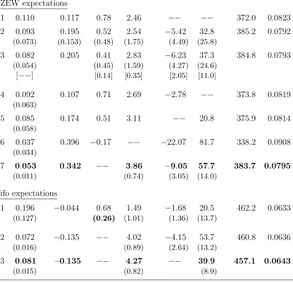
1 0.110 0.117 0.78 2.46 −− −− 372.0 0.0823

2 0.093 0.195 0.52 2.54 −5.42 32.8 385.2 0.0792

(0.073) (0.153) (0.48) (1.75) (4.49) (25.8)

3 0.082 0.205 0.41 2.83 −6.23 37.3 384.8 0.0793

(0.054) (0.45) (1.59) (4.27) (24.6)

[₋₋] [0.14] [0.35] [2.05] [11.0]

4 0.092 0.107 0.71 2.69 ₋2.78 ₋₋ 373.8 0.0819

(0.063)

5 0.085 0.174 0.51 3.11 ₋₋ 20.8 375.9 0.0814

(0.058)

6 0.037 0.396 −0.17 −− −22.07 81.7 338.2 0.0908

(0.034)

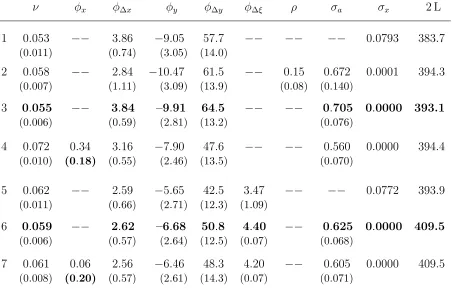
7 0.053 0.342 −− 3.86 –9.05 57.7 383.7 0.0795

(0.011) (0.74) (3.05) (14.0)

ifo expectations

1 0.196 −0.044 0.68 1.49 −1.68 20.5 462.2 0.0633

(0.127) (0.26) (1.01) (1.36) (13.7)

2 0.072 −0.135 −− 4.02 −4.15 53.7 460.8 0.0636

(0.016) (0.89) (2.64) (13.2)

3 0.081 –0.135 −− 4.27 −− 39.9 457.1 0.0643

[image:25.612.98.511.82.481.2]

(0.015) (0.82) (8.9)

Table 3: NLS estimations of the structural model (5) – (7).

Note: Numbers in parentheses are the standard errors of the estimates. Except for the first two rows in the upper part of the table, the predisposition parameter φo is

determined by condition (13),φo=φeo(φx,x¯). The lags underlying areτx= 1, τy = 4

for the ZEW index, andτx = 3,τy = 6 for the ifo index.

where c1 and c2 are two constants close to 2 that depend only on ¯x, the sample mean of

the climate index (c1 = 2 √

1−x¯√1+ ¯x, c2 = 2/[ √

(26)

This observation raises the question for the degree of nonlinearity in the structural

model. To get an impression of the curvature, two versions of the main functional expression

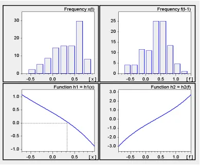
in (5) are considered, which differ in the ceteris paribus specifications to set up a one-dimensional mapping. First, we employ the estimates φo and φx from the second row of the ZEW index in Table 3, freeze y and ∆τyy at zero, and plot the graph of the function

h1 = h1(x) = (1−x) exp(φo+φxx) − (1+x) exp(−φo−φxx) (11)

This is done in the lower-left panel of Figure 2. The panel above it draws the frequency

distribution of the empirical ZEW values ofxt. It is seen in this way that at least 90 percent of the observations of xt fall into the quasi-linear segment of function h1. Things are very

[image:26.612.109.498.292.616.2]

similar if the same check is made or the ifo index.

Figure 2: Plots of the functions h1 =h1(x) and h2 =h2(f).

Note: The two top panels draw the frequency distributions of the empirical values of the ZEW indexxtand its feedback indexft−1 (derived from the estimated coefficients in row 2 of Table 3). The dotted line in the lower-left panel marks the sample mean ¯

(27)

In a second illustration, the index of the ZEW is fixed at the sample mean ¯x= 0.329. We let the entire feedback indexf vary and, in the lower-right panel in the figure, plot the function defined by

h2 = h2(f) = (1−x¯) exp(f) − (1+ ¯x) exp(−f) (12)

This function, too, is almost linear over the range that matters, as indicated by the top-right

panel that draws the frequency distribution of the empirical values of the feedback index

ft−1 in eq. (6) (likewise computed on the basis of the coefficient estimates in the second

row of Table 3). So it must be concluded from Figure 2 that the problem raised by the

relationships in (10) is indeed a relevant problem.21

3.4 Dealing with the problem of imprecise estimates

Before proceeding with the discussion, let us save one parameter. This is done for conceptual

reasons and to simplify the computations in the estimations, but it will not solve our

problem. If we have a look at the lower-left panel of Figure 2, it is seen that at the

empirical mean value of the ZEW index, ¯x= 0.329, the function h1 nearly vanishes, which

would make ¯x a point of rest in the adjustment equation (5). This observation motivates us to postulate directly that in the presence of yt−1 =∆τyyt−1 =∆τxxt−1 = 0, the sample

mean of the climate index also constitutes an equilibrium of (5). Involved are here the

two coefficients φo and φx, which, given ¯x, are linked by the condition h1(¯x) = 0 in (11).

Rearranging the terms in the equation as (1−x¯)/(1+ ¯x) = exp(−f¯)/exp( ¯f) = exp(−2 ¯f) (where ¯f = φo+φxx¯) and taking logs, the equilibrium condition can be explicitly solved

for φo. Denoting this value by a superscript ‘e’, we get

φe_o = φe_o(φx,x¯) = −

'

1 2ln

1−x¯

1+ ¯x + φxx¯

(

(13)

Technically speaking, φe

o is the intercept in the feedback index that establishes ¯x as an equilibrium point of the climate dynamics (5). Conceptually, (13) determines the

predispo-sition parameter of the agents from the average climate and the estimate ofφx. Note that the log expression is approximately (1−x¯−1)−(1+ ¯x−1) = −2¯x. Hence φe

o ≈ (1−φx) ¯x

21_{As a side result, Figure 2 ensures us that the original transition probabilities in (4),}_π−/+

t =ν exp(±ft), are well specified; given the order of magnitude of the estimated ν, the condition that they are less than

(28)

and, provided that φx is less than unity, a positive (negative) sample mean of the climate index is, in the structural model, indeed indicative of a predisposition of the agents toward

optimism (pessimism).

For a nonlinear regression it is no additional problem to replace the coefficient φo in (5) and (6) with the value of φe

o in (13) that is linked to φx. The estimation result for the ZEW index is reported in the third row of Table 3. Apparently, as a comparison with the

likelihood in the second row shows, the requirement that the conceptual equilibrium value

of x coincides with the sample mean is not a very strong constraint on the data. However, as noted before, the problem of the imprecise estimates remains.

If we therefore return to eq. (10) and follow the remark on these relationships, the most

straightforward solution seems to fix the parameterν from the outside. But at what level? It would in this respect be desirable to have some evidence, possibly by way of analogy,

from the psychological literature. Here we are left with an a priori plausibility of ν as the only criterion. Referring back to the transition probabilities in (4) and, for simplicity

and just for the moment being, taking φo = 0 and x = 0 to characterize a (hypothetical) neutral state, our most recent estimateν= 0.082 has the immediate interpretation that on average an individual agent would autonomously switch every 1/0.082 ≈ 12 months from pessimism to optimism orvice versa. This seems a reasonable order of magnitude given the kind of expectations the agents have to form, and one might even wonder if a higher or a

lower flexibility would be more plausible.22

Nevertheless, before contenting ourselves with this solution and its remaining

arbi-trariness, let us consider the other parameters in the structural model. Setting φy, φ∆y and φ∆x at some exogenous value would be even more arbitrary, while (10) suggests that putting them equal to zero would deteriorate the fit too much, sinceγy,γ∆y andβ1+τx =β2

are all significantly different from zero (cf. row 6 in Table 2). The estimations in rows 4 – 6

in Table 3 fully confirm this; apart from the fact that the outcome is of no great help for a

more precise estimate of ν, either.

22_{By fixing} _ν _{= 0}_._{082 in the estimation, the four coe}_ffi_cients _φ_x, _φ

∆x, φy, φ∆y do turn significant, as shown by the standard errors in square brackets in the third row of Table 3. In particular, the t-ratios

(29)

The last coefficient available is the coefficient φx that represents the majority effect in the herding mechanism. Again, we have no direct clue for a sensible non-zero level.

Furthermore, since it has always been a central parameter in the models in the literature

and is, so to speak, the coefficient with which it all has begun (actually, the first discussions

of this kind of theory included only ν andφx as non-zero coefficients), there is also a strong psychological barrier to let φx disappear. Equation (10), however, would allow us to do so. With the estimates from the linear regression the first relationship in (10) would read

1₋2ν _≈ 1₋νc2 ≈β1+β1+τx =β1 +β2 = 1.37−0.48. Solving it for ν yieldsν ≈0.055,

which is a presentable order of magnitude as well: here autonomous switches of an agent

would be expected to occur every 1/0.055_≈18 months.

The last row in the upper part of Table 3 shows the other coefficients and the

log-likelihood resulting from this equation. First, all of the remaining coefficients are now

highly significant. And second, if the likelihood is compared to that in the third row, then

the deterioration in the fit is insignificant. Hence, in terms of parsimony, row 7 is to be

preferred to row 3 (with ν as part of the estimation). In other words, if we start from the estimation in row 7 and then consider to introduce φx as an additional coefficient, the insufficient increase of the likelihood in row 3 would advise us against this generalization

of the model. In this sense the estimation in row 7 is optimal, which we emphasize by the

bold face characters.

To sum up, in the estimation of the structural model (5) – (7) on the ZEW expectations

index we, legitimately, decide against the majority effect and dismiss it from the model.

Herding is therefore exclusively represented by what we have called the moving-flock effect

(φ∆x >0), and in combination with the hetero-reference mechanism we settle down on the estimates presented in row 7 of Table 3.

The estimation of the ifo expectations can proceed along the same lines. The lower

part of Table 3 can thus be limited to the key results. The first row is the unconstrained

estimation (except for subjecting the predisposition parameter to the consistency condition

(13),φo =φeo(φx,x¯), where, as it should be,φo comes out negative). As opposed to what we obtained for the ZEW expectations, here the likelihood exceeds that of the corresponding

linear regression (see row 4 in Table 2); but again the difference is not significant.

Of course, the problem of imprecise parameter estimates does not disappear. It is,