Optimal bidding in Google Shopping

(1)

1

ADWORDS

ROBOT

Master’s Thesis Applied Mathematics (Chair: Stochastic Operations Research)

Faculty of Electrical Engineering, Mathematics and Computer Science (EEMCS)

Optimal bidding

in Google Shopping

Stefan Veurink

August 24, 2015

(2)

Preface

You are reading my master thesis, which is the final part of my master Applied Mathematics at the University of Twente. This project was a collaboration between the University of Twente and AdWordsRobot, a company specialised in automated online advertising. I would like to thank several people in this preface.

In the first place I would like to thank AdWordsRobot, in particular Dennis Doubovski for providing me with a very interesting assignment and the opportunity to write this thesis at the company. I am also grateful to Dennis for his help by means of the discussions we had and his supervision during the project. I thank Tiemo Kieft for his dry humour and our conversations together. In the second place, my gratitude goes to Arnoud den Boer, my supervisor at the University of Twente for his supervision. His advices have pointed me in the right directions and helped to keep the right focus during the project. I thank Richard Boucherie and Georg Still as well, for being part of the Assessment Committee and reviewing this thesis.

Finally, I would like to thank Simon Luijsterburg and Maarten Otten for reviewing my thesis and for their important feedback. I hope you will enjoy reading this thesis.

(3)

A merchant advertising products on Google Shopping has to bid on his advertisements in order for them to be shown. In this project we present a method to calculate optimal bids. When sufficient historical sales data is available, the optimal bid is calculated by estimating model parameters directly from the historical data. For products with insufficient data, we learn optimal bids using a multi-armed bandit. Furthermore, we investigate if product characteristics can be used to aggregate data such that the profit of the products increases.

(5)

Chapter 1

Introduction

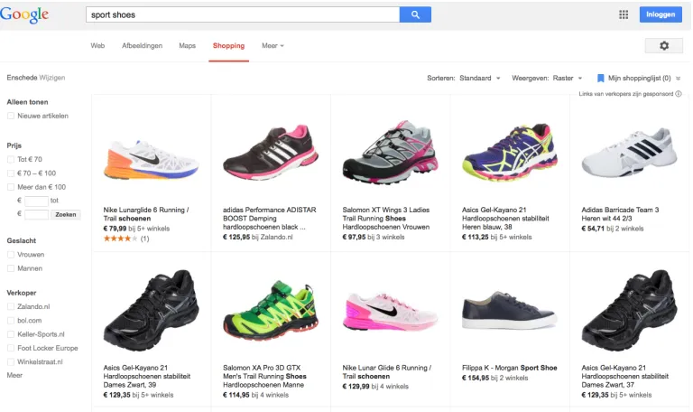
[image:5.612.116.500.344.572.2]

This master thesis is about optimisation of the bidding strategy of advertisers on Google Shopping. In the past, products were primarily sold by retailers in physical shops. Today, through the rise of the internet, many firms found new ways to sell their products. As a result, the percentage of goods sold online has been growing each year. In the US for instance, E-Commerce retail sales accounted for 6.6 % of total sales in the third quarter of 2014 (US. Bureau of the Census, 2014). Hence, online advertisement is important for online merchants to get customers to buy their products. One way to advertise products is by using Google Shopping.

(6)

1.0.1 Google Shopping

Consumers who are searching for particular products often use search engines to find web shops selling the product they are looking for. Google Shopping1 is a comparison shopping engine that provides an opportunity for a customer to compare products based on any attribute the customer is interested in; e.g. price, colour, brand, seller. See Figure 1.1 for an example. For a merchant, this is an opportunity to advertise his products.

Google Shopping started as Froogle in 2002. It started as a free service for merchants, but after several name changes the service was called Google Shopping in May 2012, alongside with the announcement that there would be a shift to paid service in late 2012 (Google Commerce, 2012). This paid service means that a merchant has to pay for each time a customer clicks on one of the merchant’s ads. This system of payment is called Pay Per Click. A customer can only click on an ad when the ad is visible for the customer, also known as animpression. To get impressions, merchants have to bid the amount they want to pay per click for each ad. Each time a customer searches for a specific product, Google holds a real time second-price auction, see Subsection 1.0.2, to decide which ads will be shown. The result of the auction depends on the heights of the bids and the relevance of the ads (Google Commerce, 2012). If the customer gets an impression of the merchant’s ad, the customer might decide toclick on the ad, which redirects the customer to the web shop of the merchant. In that case, the merchant automatically pays advertising cost to Google. The customer eventually can decide to buy one or more products, also known as aconversion. The buying process is visualised in Figure 1.2.

Merchants manage their bids in a merchant centre. In this merchant centre, bids can be set for each ad individually, or by setting bids for product groups. In the latter case, ads in the same product group get the same bid. A merchant can also decide to set a daily budget for product groups. For instance, consider a merchant with 10 products. This merchant decides to make a product group of 7 products and another product group of 3 products. For each of these products the merchant sets a budget of 50 euros. If the total cost of a group reaches 50 euros during a day, then all the bids of products in this product group are automatically set to zero. The bids of products in the other product group do not change, since each product group has its own budget.

Sales information is recorded for each product and is visible for the merchant in the merchant centre. More information about the sales information is given in Section 2.1.

1.0.2 Second-price auction

Although up to the moment of writing this thesis, Google has not been very transparent about the auction mechanism in Google Shopping, the mechanism is assumed to be similar to the mechanism in Google AdWords (Google Support, n.d.). An example is shown in Table 1.1. The AdWords auction works as follows:

Each time a customer searches for a product, an auction is held. The auction is based on Google’s AdRank, which is approximately the bid multiplied by the quality score of the ad. The quality score of an ad is mainly based on the expected click-through rate (CTR) of the ad and the attractiveness of the landing page, i.e., the web page of the web shop the customer sees after clicking the ad. The ad with the highest AdRank gets the first slot and has a Cost Per Click (CPC) equal to the second highest AdRank divided by the quality score of the ad with the highest AdRank. Similarly, the ad

(7)

Customer Searches (Query) Results in

real-time auction

Impression? Does the customer get to

see the merchant’s ad?

No cost for merchant

Profit + Cost for Merchant Conversion?

Does the customer buy 1 or more of

merchant’s products? (Bernoulli) Click?

Does the customer click on merchant’s

ad? (Bernoulli) No

Yes

Yes Yes

No

No No cost for

[image:7.612.116.499.131.354.2]

merchant Cost for merchant

Figure 1.2: Flow chart of the simplified buying process of customers on Google Shopping. The CTR is the click-through rate, which is the fraction of impressions that results in clicks. The CR is the conversion rate, which is the fraction of clicks resulting in conversions.

with the second highest AdRank gets the second slot with CPC equal to the third AdRank divided by the quality score of the second ad, etcetera. The ad with the lowest AdRank is not shown at all. The higher the quality score of the ad, the lower the CPC. When the quality scores are equal, the CPC of the ad with highest AdRank is equal to the second highest bid. Therefore this mechanism is calledsecond-price auction.

A merchant only pays the CPC when his ad is clicked on by the customer. Note that the CPC is never higher than the original bid.

Bid Quality Score Ad Rank CPC Slot

¤2 10 2∗10 = 20 12/10 =_¤1.20 1

¤3 4 3∗4 = 12 7/4 =¤1.75 2

¤1 7 1∗7 = 7 N/A No slot

[image:7.612.162.454.544.599.2]

(8)

1.1 Motivations and Research Questions

A merchant wants to maximise the expected profit of his ads, i.e. he wants to maximise the expected total profit of his products per time period. Here, the total profit is defined as the profit margin times the total sales, minus the total advertising cost.

An advertiser has several options to improve the expected profit of a product:

• Adapting the bid:

A higher bid increases the AdRank. This might result in more clicks and more conversions, resulting in a higher revenue. However, the CPC will also increase in that case, resulting in higher advertising cost.

• Improving ad quality:

Using a picture that is more attractive and has a higher resolution, choosing a more suitable, attractive title or adapting the price of the product might improve the quality of the ad. This results in a higher click-through-rate (CTR, i.e. the fraction of impressions that result in clicks), which in turn results in a higher quality score, a higher AdRank, and lower advertising cost per click (CPC).

• Improving quality of the web shop and the landing page:

An attractive landing page is crucial for getting a high conversion rate. Improving the landing page can be done for example by providing better information about price and additional costs of the product and by using more attractive pictures of higher definition. This might improve the quality score of the ad.

The scope of this paper is to improve the profit of products by adapting only the bids of the products.

Although bidding high might generate many clicks, it also results in a high CPC and a lower profit per click. On the other hand, bidding low generates only few clicks and hence low rewards. Therefore, the general research question is:

“How to determine bids on Google Shopping that maximise the total expected profit of a web shop?”

The optimal bid depends primarily on the conversion rate (i.e. the fraction of clicks that results in conversions), and the expected number of clicks as a function of the bid. Historical sales information (e.g. total sales, number of clicks, average CPC) of products is available to estimate these two metrics and subsequently determine the estimated optimal bids.

(9)

of single products. On the one hand, aggregation of data increases the sample sizes and therefore might increase the accuracy of the estimations for single products. On the other hand, aggregating data of products that have different parameters also creates biases that decreases this accuracy. Consequently, the optimal bids of products within the same bucket must lie approximately close to each other to minimise these biases.

In our data, each product has certain characteristics, such as the brand and the product type. We want to know which product characteristics are most useful to form the buckets.

Moreover, we want to know if the use of buckets can actually increase the total profit of a web shop, when compared to single product data.

Concluding, we have two sub questions, formulated as follows:

(A) What product characteristics should be used to form buckets, such that the optimal bids of products within the same bucket lie close to each other?

(B) Can we increase the total profit of a web shop by aggregating data per bucket and learning optimal bids of these buckets, instead of learning optimal bids of single products?

1.2 Related Work

Google Shopping has not been a paid service until 2012 (Google Commerce, 2012). Unfortunately, there is no relevant scientific literature about this specific topic at the moment of writing this thesis, probably caused by the young age of this platform. Nevertheless, there is a vast amount of literature about other forms of sponsored search (i.e. paid search), which has been a marketing opportunity since the beginning of this century. Although this literature can give valuable insights for our project, there are some important differences to notice between general sponsored search and Google Shopping.

Often in sponsored search, advertisers bid on keywords and the corresponding problem is to identify appropriate keywords that match with the search queries to their offered products or services, and subsequently determine the optimal bids on those keywords (Even Dar, Mirrokni, Mutukrishnan, Mansour & Nadav, 2009). Matching keywords with search queries is done using “broad match” or ”exact match”. Broad matching means that an advertiser targets a large number of related queries while bidding only on a limited number of keywords. Exact matching means that only queries that are exactly the same as the keywords are targeted. The chosen matching option has a significant influence on keyword performance (Klapdor, Anderl, von Wangenheim & Schumann, 2014). In contrast to general sponsored search, in Google Shopping, advertisers bid on products and matching products with search queries is done by Google instead of by the advertiser itself. Setting optimal bids is the problem that remains for the advertiser.

Another difference is that in general sponsored search, historical information about the average rank of ads is often given to advertisers by the marketing platform owner. The rank of ads is very important for the number of clicks that ads receive. However, the interface of ads in Google Shopping is very different than in general sponsored search and Google does not provide information to advertisers in Google Shopping about the average AdRank of their ads.

(10)

(Zhou, Chakrabarty & Lukose, 2008; Feldman, Muthukrishnan, P´al & Stein, 2007; Borgs, Chayes, Immorlica, Jain, Etesami, & Mahdian, 2007; Chaitanya & Narahari, 2012; Pin & Key, 2011). In our research, we regard the perspective of the advertiser and for simplicity, we assume static behaviour of competing advertisers. In other words, we assume that other advertisers do no adapt their bids to our bidding strategy.

Several papers analyse the problem of selecting optimal keywords to bid on given a budget con-straint. Rusmevichientong & Williamson (2006) provide an algorithm that adaptively identifies the set of keywords that maximises the expected profit, based on historical performance given a fixed daily budget and unknown click-through rates. The algorithm they use is an adapted multi-armed bandit. However, they assume the reward per click of each ad is known, while in practice this parameter is unknown. Feldman et al. (2007) use a strategy with a uniform bid on all keywords to maximise the number of total clicks on the ads, given a fixed budget. In order to maximise the profit given a budget, Borgs et al. (2007) equalize the return-on-investment (ROI) across all keywords together with some random perturbations to prevent cyclic behaviour. In our work, we analyse optimal bids of products without any budget constraints.

Two important metrics in sponsored search are the click-through-rate (CTR) and the conversion rate (CR), which are both proportions. Research has been performed to predict the CTR of ads. For example, Regelson & Fain (2006) predict the CTR of low-volume search terms and terms with-out historical information. Using hierarchical clusters of related terms, they achieve 40-43% more accurate estimates than broader estimates for terms without historical information. Richardson, Dominowska & Ragno (2007) predict the CTR of new ads by analysing the variance of the CTR across terms and the variance of the CTR within a term using logistic regression. They achieve a 30% error reduction compared to the estimate using the general CTR in their training set. In-formation about the CTR is most important for the auctioneer, who wants to show the ads that generate the most clicks in order to maximise its revenues and improve user satisfaction. Although predicting the CTR is important for advertisers as well, predicting the conversion rate (CR) is more important. In the current work, learning the CR of a product is necessary in order to optimise the bids.

Using logistic regression, Ghose & Yang (2009) find that incorporating advertiser names in an ad increases both CTR and CR, while brand names decrease the performance of these metrics. Al-though this conclusion is drawn for brands in general, positive effects might hold for specific popular brands. These results were strengthened by Klapdor et al. (2014) using multiple regression. The latter also define a query-variation index that measures the extent to which a keyword is information specific. This index was found to be a good predictor of the CTR and the CR as well.

(11)

A. General model

B.MIP conditions:

Sufficient data of a product?

Calculate optimal bid using general model

D. MAB:

Learn optimal bids using a multi-armed

bandit (MAB)

D1. Individual method:

Bid on individual products

D2. Bucket method:

Bid on buckets of products using aggregated data

Yes

No

C. Decision tree:

Form buckets using conditional inference tree

APPROACH

[image:11.612.172.462.97.331.2]

Keep learning from generated data

Figure 1.3: General approach

1.3 Approach

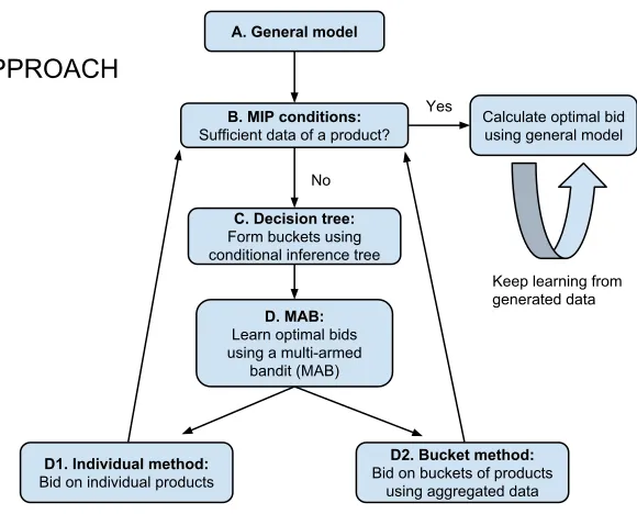
Our approach to learn optimal bids is visualised in Figure 1.3. First, we develop a general model (A) to calculate optimal bids of products with sufficient data. However, the majority of products does not possess sufficient data to directly use the model. Therefore, we define two categories of products based on the amount of historical sales data of each product (B). All products with sufficient amount of historical sales data are defined as the Much Information Products (MIP). Similarly, all other products are defined as the Few Information Products (FIP). In Section 2.3 we give more detailed conditions defining these two categories.

For each MIP product, we calculate the optimal bid using the general model. The optimal can be updated periodically in order to keep learning from newly generated data. For FIP products, we choose to learn optimal bids using a multi-armed bandit (MAB) (D), explained in Section 2.5. In the context of optimal bidding, we face a trade-off between placing the bid that is expected to give the highest profit (we will call thisexploitation), and trying other bids to receive more information about their expected profits (we will call thisexploration). Bandits provide a learning mechanism that balances exploration and exploitation in order to maximise the total profit over a certain period. Especially for products that contain few historical data, incorporating an exploration part is important to increase the long-term profit. In order to get answers to the sub questions of this project, we analyse two methods.

(12)

according to the MAB algorithm. This results in a different bid for each product. Correspondingly, each product learns its optimal bid.

The second method, the bucket method (D2), does not directly learn the optimal bids of products. Instead, optimal bids are learned per bucket of products, by using the aggregated data of similar products. By aggregating the data, the estimates of the model parameters might be closer to the true values than using the individual method.

Reward per click

Frequency

0 5 10 15 20

0

100

200

300

400

[image:12.612.195.398.208.396.2]

500

Figure 1.4: Histogram of the reward per click of all products in the data set.

The buckets are formed using a decision tree algorithm (C). To be precise, we use a conditional inference tree. We give several reasons why we choose this algorithm.

The underlying problem that sub question A points to, is the problem of determining product characteristics that predict the optimal bid of products. Moreover, since the optimal bid of a product is a continuous variable, this is a regression problem. Unsupervised learning algorithms, such as a clustering algorithm, could be used to split up our product set into several clusters, or buckets, such that products within each bucket have similar optimal bids. However, this does not give information of product characteristics that are predictors of the optimal bid. Hence, unsupervised learning algorithms are not suitable. On the other hand, although well-known regression models, such as (generalised) linear models and logistic regression, provide a way to determine predictors, they do not form buckets.

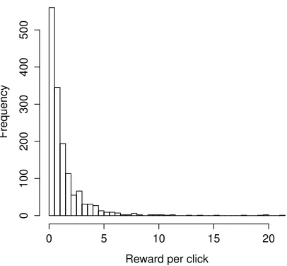
Decision trees provide a way to split the product set into buckets of similar products with similar bids, based on their product characteristics. Also, decision trees are simple to understand and do not assume a parametric distribution of the response variable. The latter property is particularly useful in the context of this project, considering the skewed distribution of the reward per click, see Figure 1.4.

(13)

splits are prevented (Hothorn, Hornik & Zeileis, 2006). Some of the nominal variables in our data have many levels. The statistical approach of the conditional inference tree helps to determine splits of the training set that can be generalised to other sets, instead of splits that are found by chance. Other decision trees have more difficulties with this issue.

1.4 Structure of the Report

(14)

Chapter 2

General model & Algorithms

The general purpose of this chapter is presenting the general model we developed together with the algorithms we use, as a means to increase the total profit of a web shop. We start this chapter with presenting the data and its characteristics. This section is followed by the mathematical model and estimation techniques to estimate the two key parameters of the model. Subsequently, we discuss two algorithms. The first algorithm is the decision tree algorithm to split a set of products into buckets of products. The second algorithm is the multi-armed bandit algorithm to learn optimal bids of single products (i.e. the individual method) or optimal bids of buckets (i.e. the bucket method).

2.1 Data

Each merchant advertising on Google Shopping is provided by Google with historical sales infor-mation of his products at the days the merchant was active on the marketing platform. For this project, the sales information of some merchants is available. The data of each merchant is put together in a data frame, where each row has around 26 columns representing the sales information of a single product on a particular day along with some product characteristics. A data snippet of the data set is visible in Figure 2.1a. The sales information contains the number of impressions, clicks and conversions generated by that product on that day, together with the paid advertising cost for the product. The product characteristics are the brand, product categories, product types and possibly any custom labels of the product, all provided by the merchant to Google. Our data contains this information.

In addition, the price of the products are given.

Finally, we emphasize that no data is available of placed bids on products. This means we are not able to estimate a direct relationship between the bid and the expected number of clicks.

2.1.1 Data set

The data set is from a merchant selling outdoor articles such as scooters, skates, shoes, etcetera. The time period of this data set is 11 March 2014 to 4 February 2015.

(15)

[image:15.612.99.516.93.370.2]

(a) Data snippet (b) Number of levels of each factor

Figure 2.1: Some information of the data set.

together with their associated number of levels, i.e. the number of different values of each factor. For instance, the factor ’Brand’ has 414 levels (e.g. ’urbanears’). The factors containing ’Custom.label’ are ignored in the analyses, due to the many empty cells in these columns or due to the information in these columns being the same as in other columns. There is a total of 14,003 products in the data

Products with Clicks Products without Clicks Total

Products with Conversions 1,489 0 1,489

Products without Conversions 7,116 5,398 12,514

Total 8,605 5,398 14,003

Table 2.1: Statistics of the data set.

[image:15.612.98.517.481.536.2]

(16)

2.2 General Model

This section describes how to determine optimal bids of products with sufficient data by estimating model parameters. This is part A of our approach as visualised in Figure 1.3.

Since the data is given per day, the standard time period we use in our model is a day. The profit per day, V, is a function of the cost per click, κ. V is modelled as the number of clicks per day,

C, times the profit per click. The profit per click is the difference between the reward per click, R, andκ. The reward per click,R, equals the conversion rate (i.e. the probability a click results in a conversion), times the conversion reward. The conversion reward is equal to the average sales value times the profit margin.

In practice, the merchant sets the bid and thenκis a random variable that is always lower than the bid, since Google Shopping works with second-price auction. However, there is no information about the placed bids in the data, see Section 2.1. Therefore, we use the cost per click κ as a proxy for the bid price. This was done by Ghose & Yang (2009) as well. In addition, we assume we are able to setκas a decision variable. The optimal cost per click,κ∗, is defined as theκthat maximises the expected daily profit.

In formula:

E[V(κ)] =E[C(κ)]∗(R−κ) (2.1)

κ∗= arg max

κ E

[V(κ)] (2.2)

2.2.1 Number of clicks as a function of the average cost per click

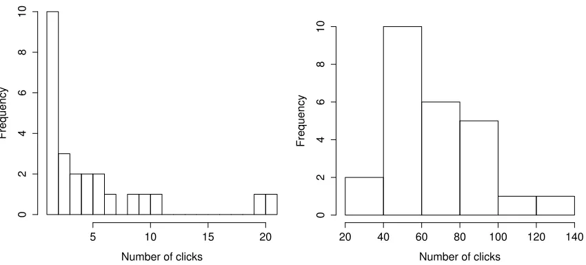
In Figure 2.2, two histograms are shown of the historical number of clicks per day of a specific product in the data set. In Figure 2.2a, only the data records with an average cost per click between ¤0.20 and ¤0.30 are used. In contrast, Figure 2.2b shows the histogram of the data records with an average cost per click between ¤0.80 and ¤1.00. Both figures show the typical positive skew in the distribution of the number of clicks given a fixed cost per click. Moreover, the skewness of the distribution seems to be decreasing when the average cost per click is increasing. Given a constant bid, we assume that clicks on a specific ad occur with a constant rate per time unit (e.g. per day). For simplicity of the model, we assume no seasonality, which means that the arrival rate does not change over time. Furthermore, we assume that customers behave independently of each other. Hence, the inter-arrival times of clicks are mutually independent. Also, we observe that the higher the average cost per click, the higher the arrival rate of clicks.

To incorporate the skewness of the distribution of the daily number of clicks and aforementioned assumptions, we assume that the number of clicks generated by a specific product in a fixed time interval, given a fixedκ, has a Poisson distribution with rate λ(κ):

C(κ)∼Poisson(λ(κ))

(17)

Number of clicks

Frequency

5 10 15 20

0

2

4

6

8

10

(a) Average cost per click between_¤0.20 and_¤0.30.

Number of clicks

Frequency

20 40 60 80 100 120 140

0

2

4

6

8

10

[image:17.612.94.519.122.314.2]

(b) Average cost per click between_¤0.80 and_¤1.00.

Figure 2.2: Histograms of the historical number of clicks per day of a specific product, conditioned on a certain range of the average cost per click. In order to be able to calculate the average cost per click, only data records with non-zero number of clicks were used.

calculated when the number of clicks is non-zero in a data record. Using normal Poisson regression would yield too high estimates ofλ. To circumvent this bias, we use zero-truncated Poisson regres-sion (Cohen, 1960). We choose the natural logarithm ofκas the only predictor. Since the natural logarithm is the standard link function for Poisson regression, we use it also as the link function between the expected number of clicks and the predictor. Hence, we get:

ln(_E[C(κ)]) = ln(λ(κ)) =α+β∗ln(κ) (2.3)

and

C(κ)∼Poisson(λ=eα+β∗ln(κ)), k∈(0,∞)

In the latter equation, model parametersαandβ are estimated by ˆαand ˆβ, respectively. λcan be written asλ=eα_∗_κβ_{. This reveals that parameter}_β _{can be seen as a shape parameter, while} _α

quantifies the relative magnitude, compared toλ(κ) of other products.

(18)

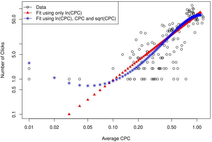
Firstly, asκgoes to zero, λ(κ) goes to zero. This is a property ofλ(κ) that needs to hold, since the number of clicks goes to zero when the placed bid goes to zero. Therefore, we require ˆβ to be positive. Secondly,λ(κ) is non-decreasing in κ, reflecting the fact that a bid never generates less clicks than a lower bid. Figure 2.3 shows that adding other predictors such asκor √κdoes not always result in a regression fit that has this two properties.

0.01 0.02 0.05 0.10 0.20 0.50 1.00

0.1

0.5

1.0

5.0

50.0

Average CPC

Number of Clicks

Data

Fit using only ln(CPC)

[image:18.612.115.481.204.450.2]

Fit using ln(CPC), CPC and sqrt(CPC)

Figure 2.3: Number of clicks (black circles) as a function of the average cost per click κ, plotted together with two regression fits on a log-log scale. Data is from the product with the most historical clicks in the data set. The fit using only ln(κ) (red triangles) as predictor is non-decreasing, while the fit where predictorsκand√κare added (blue asterisks) is not non-decreasing.

2.2.2 Estimating conversion rate

(19)

rate equal to zero is not realistic. Lewis & Sauro (2006) demonstrate that the best point estimator to use in these extreme cases is the Laplace method (Laplace, 1812). Therefore, we estimateρusing this method, which adds 1 success and 1 failure:

ˆ

ρ= Historical total number of conversions + 1 Historical total number of clicks + 2

2.2.3 Calculating the optimal cost per click

When bothλ(κ) andρare known, we can calculateκ∗_{of a product using Equation 2.1, Equation 2.2} and Equation 2.3. We have:

E[V(κ)] =E[C(κ)]∗(R−κ)

=eα+β∗ln(κ)∗(R−k) Taking the derivative with respect toκwe get:

d

dκE[V(κ)] = β κ∗e

α+β∗ln(κ)

∗(R−κ)−eα+β∗ln(κ)

=

(_β_∗₍_R₋_κ₎

κ −1 )

∗eα+β∗ln(κ)

Setting the derivative to zero results in:

β∗(R−κ) =κ

κ∗(β+ 1) =β∗R

As a result, the optimal cost per click is:

κ∗= β

β+ 1 ∗R (2.4)

The second derivative ofE[V(κ)] is equal to:

d2

dκ2E[V(κ)] =

(_−κ_∗_β₋_β_∗₍_R₋_κ_{) +}_β2_∗₍_R₋_κ₎₋_κ_∗_β

κ2

)

∗eα+β∗ln(κ)

=β∗ (

−κ∗(β+ 1)−R∗(1−β)

κ2

)

∗eα+β∗ln(κ)

Filling inκ∗_{, the nominator of latter equation becomes:}

−κ∗∗(β+ 1)−R∗(1−β) =− β

β+ 1∗R∗(β+ 1)−R∗(1−β)

=−R <0

Given a positiveβ, the second derivative of_E[V(κ)] is negative inκ∗. Hence, _β₊₁β ∗Ris indeed the optimal cost per click.

(20)

2.3 MIP conditions

The previous section shows how to estimate model parameters in order to calculate the optimalκ

for a product. However, this is only valid if model parameters are known or can be estimated with sufficient reliability. Since the majority of products in our data has estimates with high variance, we define two categories of products. More precisely, we define a product as a Much Information Product (MIP) if the following conditions are met:

i) ρU CB<2∗ρˆandρLCB>0.5∗ρˆ

ii) Regression coefficient estimate ˆβ >0

iii) The p-value of ˆβ should be lower than the significance level of 5%.

where ρLCB and ρU CB in condition i) are the lower and upper bound of the 95% binomial

con-fidence interval of ρusing the adjusted-Wald method. This method is chosen for its good actual coverage probabilities when sample sizes are small and binomial proportions close to zero (Agresti & Coull, 1998; Sauro & Lewis, 2005). Condition i) ensures that with a confidence of 95%, the true conversion rate ρis maximally a factor two higher or lower than the estimate ˆρ. Since we have reward per clickR=ρ∗p, the trueR is then also maximally a factor two higher or lower than the estimate ofR.

Conditions ii) and iii) are to ensureλ(κ) is increasing and to ensure a certain quality of the regres-sion fit to estimateλ(κ), respectively.

Checking if a product meets the MIP conditions is part B of our general approach, see Fig-ure 1.3.

However, only a small proportion of all products meets this conditions (i.e. only 78 out of 14,003 products in the data set). All other products are defined as Few Information Products (FIP). To learn optimal κ’s of the FIP products, we use a multi-armed bandit algorithm, explained in Section 2.5. Different variants of the MAB algorithm give different values of total profit of the FIP products. To find answers to the sub-questions of this research, two MAB methods are investigated in this project.

In the first method, the individual method, we optimise the bid of each product separately by only using the generated data of the product itself. As a result of this, each FIP-product learns its own model parameter values and correspondingκ∗.

In the second method, the bucket method, we optimise theκof each bucket by using the aggregated data of all products in that bucket. Model parameters are estimated per bucket. For instance, consider a bucket containing all products with a selling price higher than¤200. We estimate the conversion rate of the bucket by using the sum of conversions and the sum of clicks of all products with a selling price higher than¤200.

2.4 Conditional Inference Tree

(21)

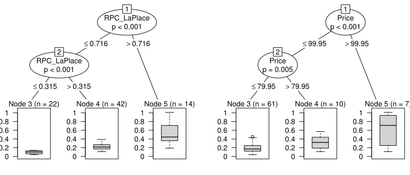
characteristics and historical sales data. However, the number of MIP products, of which theκ∗can be calculated, is relatively small. Since the optimal cost per click is perfectly correlated with the reward per click, we use the reward per click of the products as the response variable. More precisely, we build a regression tree using the Conditional Inference Tree algorithm, developed by Hothorn, Hornik, & Zeileis (2006). This algorithm is a recursive binary partitioning in a conditional inference framework. The algorithm uses permutation tests, developed by Strasser and Weber (1999), to test both the global null hypothesis of independence between any of the explanatory variables and the response variable, and the partial null hypotheses. Since the algorithm utilizes permutation tests, the response variable is not needed to be normally distributed. In addition, the use of the conditional inference framework prevents over-fitting and also prevents a bias of selecting explanatory variables with many possible splits. Other decision trees use pruning to solve the problem of over-fitting, while the problem of a selection bias towards explanatory variables with many possible splits remains. Another advantage of this algorithm is that it allows the use of both numeric variables as well as nominal variables at the same time. Hence, it provides us the opportunity to use both the price of products, a numeric variable, and the other product characteristics such as brand and product category, which are nominal variables. An example of a conditional inference tree is given in Figure 2.4.

Further details of the conditional inference tree algorithm and the permutation tests are out of the scope of this project. For the interested reader, we refer to Hothorn et al. (2006) for more information about conditional inference trees and to Strasser & Weber (1999) for more information about the permutation tests.

RPC_LaPlace p < 0.001

1

≤0.716 >0.716

RPC_LaPlace p < 0.001

2

≤0.315 >0.315

Node 3 (n = 22)

0 0.2 0.4 0.6 0.8 1

Node 4 (n = 42)

0 0.2 0.4 0.6 0.8 1

Node 5 (n = 14)

0 0.2 0.4 0.6 0.8 1

(a) With reward per click

Price p < 0.001

1

≤99.95 >99.95

Price p = 0.005

2

≤79.95 >79.95

Node 3 (n = 61)

0 0.2 0.4 0.6 0.8 1

Node 4 (n = 10)

0 0.2 0.4 0.6 0.8 1

Node 5 (n = 7)

0 0.2 0.4 0.6 0.8 1

[image:21.612.109.515.363.537.2]

(b) Without reward per click

(22)

2.5 Multi-Armed Bandit

This section starts with explaining the general idea of a MAB, part D of our general approach (Figure 1.3). Subsequently, we present an adjusted UCB1 algorithm, a well-known MAB, adjusted to increase the learning rate of the algorithm. We use this algorithm in the individual method as well as in the bucket method, respectively part D1 and D2 of our general approach.

The general idea of a MAB is a gambler playing a bandit (slot machine) with multiple arms for a finite number of rounds. Each round the gambler pulls 1 arm giving a stochastic reward. Each arm has a different reward distribution function, which is unknown to the gambler at the start. The goal of the gambler is to maximise his total expected reward over all rounds. This results in a trade-off between exploitation (i.e. choosing the arm that is expected to generate the highest reward) and exploration (i.e. choosing an arm to learn more about its reward distribution), in order to maximise the total profit over all rounds.

In the current project, we are facing an equivalent trade-off for FIP-products. More precisely, we have to balance between achieving more information about expected profits by trying different bids, and exploitation the current information by bidding the amount with highest expected profit. Therefore, bandits are particularly suitable for this problem.

2.5.1 Adjusted UCB1 algorithm

We choose to use the UCB1 algorithm (Auer, Cesa-Bianchi & Fischer, 2002) due to its simplicity. In the rest of this paper, we refer to this algorithm as the original UCB1 algorithm. The algorithm is part of the upper confidence bound algorithms. This means that confidence intervals are created for the reward of each arm and in each round the arm with the highest upper confidence bound is chosen. The UCB1 algorithm works as follows:

• Assume there areK arms andn rounds. In this project, the arms are the differentκ’s and each round is a day.

In the firstK days, eachκis tried once. This is a pure exploration phase.

• For allt=K+ 1, . . . , n, play armj that maximizes ˆVj(t) +

√_α

ucb∗ln(t−1)

Tj(t) , whereTj(t) is the number of times armj has been played up to and including timet−1. Further, αucb is an exploration parameter that can be adjusted depending on the amount of exploration that is wanted.

In the original UCB1 algorithm, ˆVj(t) is the average profit per product obtained from arm j up

to and including timet−1. However, we propose to adjust ˆVj(t) in the following way. We use a

similar formula to the one given in Equation 2.1. More precisely, we use:

ˆ

Vj(t) = ˆCj(t)∗( ˆR(t)−κj)

where ˆCj(t) is the estimated expected number of clicks per product generated by armj up to and

(23)

is the same for all arms. Since the expected reward per click is the conversion rate multiplied by the expected reward per conversion, we have:

ˆ

Vj(t) = ˆCj(t)∗( ˆρ(t)∗pˆ(t)−κj) (2.5)

where ˆρ(t) is the estimated conversion rate and ˆp(t) is the estimated expected reward per conver-sion.

We choose to adjust the original UCB1 algorithm, in order to exchange information between different arms. By the assumptions of a constant conversion reward and a conversion rate that is independent of the arm (i.e. the cost per click), we can use the aggregated number of clicks and conversions over all arms to estimate the reward per click. The original UCB1 algorithm uses the average profit of each arm, thereby neglecting the information of the conversion rate learned by other arms. In order to see if the adjusted UCB1 algorithm indeed outperforms the original UCB1, we do simulations with both the original UCB1 and the adjusted UCB1.We do this for both the individual method and the bucket method. Hence, we simulate four different methods in total.

2.5.2 Individual method

We consider a single product.

In the individual MAB method, we use only the historical information of this product and do not aggregate any information to estimate the parameters of Equation 2.5.

Conversion rate ρ is learned by using the historical information combined with the information generated during the MAB period. Since the highest estimated conversion rate of the MIP products in the data set is 0.147, we assume that a trueρgreater than 0.15 is not realistic. Therefore,ρ(t) is estimated by the minimum of the Laplace point estimate at timet and 0.15:

ˆ

ρ(t) = min{ convhist+ convMAB(t) + 1

clickshist+ clicksMAB(t) + 2 , 0.15} (2.6)

where convhist and clickshist are the historical number of conversions and clicks, respectively. convMAB and clicksMAB are the total number of conversions and clicks, respectively, generated by the single product during the MAB period up to and including timet−1.

The expected reward per conversion ˆpis assumed to be equal to the profit margin times the price of the product. Both the profit margin and the price are known in advance.

For the individual MAB method we further use that:

ˆ

Cj(t) =

clicksj(t)

Tj(t)

where clicksj(t) is the number of clicks generated by the single product using arm j, up to and

(24)

Notice that in contrary to the conversion rate estimation, no historical information is used to es-timate the expected number of clicks of each arm. By definition, most FIP products do not have enough historical information for a significant fit of estimated regression coefficient β in Equa-tion 2.3. As a result, the expected number of clicks of each arm is hard to estimate based on historical data and therefore it is not used.

2.5.3 Bucket method

In the bucket MAB method, we estimate the same parameters for products in the same bucket. The conversion rateρof a bucket is estimated using both historical information of all products in the bucket as well as the information generated by products in the bucket during the MAB period. Similarly to the individual MAB method we do not allow the estimated conversion rate to be higher than 0.15:

ˆ

ρ(t) = min{ bucket convhist+ bucket convMAB(t) + 1

bucket clickshist+ bucket clicksMAB(t) + 2

, 0.15} (2.7)

where bucket convhist and bucket clickshist are the total number of conversions and the total num-ber of clicks, respectively, generated historically by all products of the bucket.

bucket convMAB(t) and bucket clicksMAB(t) are the total number of conversions and the total num-ber of clicks, respectively, generated by the bucket during the MAB period up to and including timet−1.

Similarly to the individual method, no historical information is used to calculate the expected number of clicks per product:

ˆ

Cj(t) =

clicksj(t)

Tj(t)

where clicksj(t) is the average total number of clicks per product generated by the bucket using

armj, up to and including timet−1 of the MAB period.

The expected reward per conversion of a bucket is estimated as follows. If there has not been a conversion of one of the products in the bucket up to and including timet−1 of the MAB period, then the reward per conversion is estimated by the profit margin times the average price of the products in the bucket. Otherwise, ˆp(t) is equal to the average reward per conversion received up to and including timet−1 of the MAB period:

ˆ

p(t) = {

γ∗pbucket if bucket convMAB(t) = 0 rbucket(t)

bucket convMAB(t) otherwise

whereγis the profit margin,p_bucket is the average price of the products in the bucket andrbucket(t)

(25)

Chapter 3

Numerical Results

General model MIP conditions:

Sufficient data of a product?

FIP - products

Yes

TEST

Perform simulations:

Individual method:

Bid on individual MIP-products

Bucket method:

Bid on buckets of MIP-products using aggregated

data

Decision tree:

Form buckets using conditional inference tree

with FIP-products

MIP - products

[image:25.612.153.427.255.488.2]

No

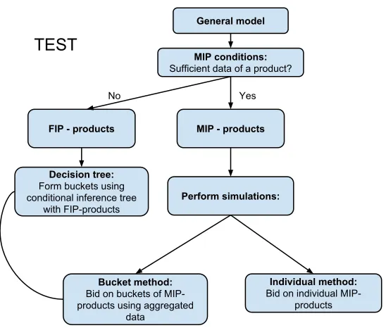
Figure 3.1: Test procedure

In order to determine which MAB method is better we test the performance of both the individual method as well as the bucket method using simulations. The procedure is visualised in Figure 3.1. After we have categorised all products into MIP and FIP products, we choose the MIP products as validation set. By definition, for these products we have model parameter estimates with rela-tively small variance. Accordingly, we expect to get more realistic simulations than using arbitrary products.

To prevent a bias in the results of the simulations, we use the FIP products as the training set of the decision tree algorithm.

(26)

seen as new products. However, in the bucket method, we use the aggregated historical information of the FIP products.

In the data set there are 78 MIP products (i.e. products that meet the conditions in Section 2.3). These products have generated 41% of the total number of conversions, 25% of the total number of clicks, 16% of the total number of impressions and 38% of the total cost of the data set. In order to form the buckets, we built a conditional inference tree using the reward per click (RPC) as the response variable. The training set used to built the tree are all FIP products that have historically generated at least 1 conversion (i.e. 1,411 products). We do not include the MIP products when building the tree, to prevent the creation of bias in the results of the bucket MAB simulations. We use 8 predictors: 7 factors as explained in Subsection 2.1.1, together with the price. Thereby, we restrict the buckets to contain a minimum of 5 FIP products.

[image:26.612.91.522.262.599.2]

After running the algorithm, a tree is built with 13 inner nodes and 14 terminal nodes, which means 14 buckets are created. A print of the tree is shown in Figure 3.2.

(27)

For instance, bucket 12 contains all products for which the following conditions on the product characteristics hold:

• Selling price between¤17.475 and¤34.95,

• Category..3rd..level. is an element of the set{, Athletic Shoes & Sneakers, Riding Scooters, Skateboarding, Skating, Skiing},

• Category..1st..level. is an element of the set{, Clothing & Accessories}

Although the first comma in both category sets seems useless, it represents all products with no value for this product characteristic in the data.

Now the decision tree is built, we are able to see which product attributes are the best predictors of the RPC. At each of the 13 inner nodes, a set is split into two subsets based on the predictor with the strongest association with the RPC. For example, at inner node 1, the total set of FIP products is split based on the price. Products with a price higher than_¤81.40 are separated from products with a price lower than_¤81.40. This is the split at the highest depth level of the tree, level 1. It indicates that price is a stronger predictor than the other predictors. To get an idea of the strength of each predictor, we sum the numbers of splits at each depth level for each predictor, shown in Table 3.1.

Predictor # Level 1 # Level 2 # Level 3 # Level 4 # Level 5

Splits Splits Splits Splits Splits

Price 1 1 3 2 1

Product type 1 0 0 0 0 0

Brand 0 0 0 1 0

Category 1 0 0 0 0 1

[image:27.612.128.485.319.444.2]

Table 3.1: Number of splits per depth level of the tree, per predictor.

Clearly, the price is the strongest predictor of the 8 given predictors. The second best predictor seems to be category 4, which accounts for splits on the second and third depth level of the tree. Surprisingly, the brand of products does not seem to be a strong predictor, although it accounts for one split at depth level 4.

Using the splits of this tree, we split the 78 MIP products into 8 buckets (i.e. 6 buckets do not contain MIP products) based on their product characteristics. The number of MIP products per bucket is shown in Figure 3.3. The numbers of the buckets are the numbers of the corresponding terminal nodes of the decision tree.

Two of these buckets only contain 1 MIP product. Since there is no difference between the individual and the bucket method for a bucket with only 1 product, we do not analyse these two products. As a result of this, 6 buckets containing a total of 76 MIP products are left over for analysis.

(28)

[image:28.612.271.341.91.222.2]

Figure 3.3: Total number of MIP products (right column) per bucket (left column). The bucket numbers are the numbers of the corresponding terminal nodes of the decision tree.

Bucket.8 Bucket.12 Bucket.13 Bucket.19 Bucket.20 Bucket.26

Number of MIP products 2 2 14 12 30 16

Summary statistics of κ∗

Minimum 0.08 0.04 0.05 0.06 0.06 0.11

1st Quantile 0.10 0.10 0.11 0.19 0.12 0.23

Median 0.11 0.16 0.14 0.22 0.18 0.32

Mean 0.11 0.16 0.15 0.24 0.19 0.42

3rd Quantile 0.12 0.22 0.18 0.27 0.25 0.50

Maximum 0.14 0.28 0.29 0.45 0.43 1.01

Coefficient of Variation 0.39 1.06 0.48 0.46 0.48 0.70

Table 3.2: The number of MIP products and several summary statistics ofκ∗, per bucket. The bucket numbers are the numbers of the corresponding terminal nodes of the decision tree.

width of the buckets is also reasonably large. For instance, the smallest coefficient of variation is 0.39, which means that the standard deviation is almost halve of the mean value.

Next, we treat these 76 MIP products as if they were new products. More precisely, to test the individual method we set convhist and clickshist in Equation 2.6 equal to zero. To test the bucket method, we set bucket convhist and bucket clickshistin Equation 2.7 equal to the historical number of conversions and clicks of the FIP products belonging to the corresponding bucket.

We perform 2000 iterations of both the individual method and the bucket method using the adjusted UCB1 algorithm. In addition, we simulate both methods using the original UCB1 algorithm as well. In the MAB algorithms, we have to choose several parameters.

Firstly, we choose to run both algorithms using 100 rounds (i.e. 100 days), since a longer period would not be realistic.

[image:28.612.93.555.263.389.2]

(29)

arm (in our analysis this is_¤0.50) should preferably be set depending on the expected RPC of the product. In the discussion we come back to this.

In the exploration term √

αucb∗ln(t−1)

Tj(t) , parameter αucb is set equal to 0.3, since this results in a range of the exploration term from 0.12 (arm pulled 91 times after 100 days) to 1.18 (arm pulled only once after 100 days). These values approximate the mean and median values of the optimal daily profits of the MIP products, which are 1.04 and 0.60, respectively. Hence, by settingαucbto 0.3, we try to balance the exploitation and exploration.

3.1 Total Results

In total we simulated four different methods. For each method we calculate the daily product regret for each product, averaged over 2000 iterations. Here, the regret is the difference between the actual profit and the maximal achievable expected profit. In other words, this is the expected extra profit that we would have achieved if the optimal cost per click was paid. The maximal achievable expected profit is calculated using Equation 2.4. Notice that zero regret is not attainable using our MAB, due to the fact that the arms are discrete, while the optimal cost per clickκ∗is continuous. By summing the daily product regret of the 76 MIP products we get the daily total regret for each day x, for all x∈ {1, . . . ,100}. The results of each method is plotted in Figure 3.4.

Next, we calculate the sum of these daily total regrets to get the period cumulative regret from day 1 up to day x, for all x∈ {1, . . . ,100}. These results are shown in Figure 3.5.

We expected to see that the bucket method using the adjusted UCB1 algorithm would achieve lower regrets in the first days after the exploration phase as a result of using aggregated data. However, these figures show that the individual method using the adjusted UCB1 algorithm achieves lower regrets than the bucket method using the adjusted UCB1. The figures show that the original UCB1 algorithm is outperformed as well. In the first 10 days, the exploration phase, the four methods are exactly the same, and the plots show that their performance is also approximately the same. After 10 days, when the exploration phase ends, the plot of the individual method diverges directly away from the other plots.

Further, we see extreme high regrets in the last few days of the exploration period. Since these are the arms with the highest cost per click, this indicates that the cost per click corresponding to these arms are too high. The part of the MIP products that account for the majority of the total revenue has aκ∗ that is much lower then _¤0.50. More precisely, 80% of the MIP products has a

(30)

0 20 40 60 80 100

0

50

100

150

Day

Daily T

otal Regret

[image:30.612.165.435.120.304.2]

Individual method (adjusted) Bucket method (adjusted) Individual method (original UCB1) Bucket method (original UCB1)

Figure 3.4: Progress of the daily total regret for both methods in euros (y-axes) over time (x-axes). The individual method using the adjusted UCB1 algorithm (red open circles) clearly achieves lower regrets than the other methods.

0 20 40 60 80 100

0

500

1000

1500

2000

2500

3000

Day

P

er

iod T

otal Regret

[image:30.612.164.437.385.565.2]

(31)

3.2 Results per bucket

In order to get more detailed insights into the results, we plot the progress over time of the period regret and daily regret, per bucket. These results are shown per bucket in Figure 3.6 and Figure 3.7. Table 3.3 shows the period cumulative regrets in numbers for bucket 20, as an example. In the last column of this table the optimal profit up to each day is given. Recall that the regret is the difference between the achieved profit and the optimal profit.

Day Individual Bucket Individual Bucket Optimal profit

Adjusted Adjusted Original Original

Exploration

1 11.43 11.75 11.57 11.63 22.51

2 18.13 18.91 18.51 18.88 45.02

3 23.00 23.22 23.72 23.62 67.54

4 28.00 29.25 29.07 28.63 90.05

5 34.94 36.26 36.00 36.65 112.56

6 47.33 49.46 48.97 49.62 135.07

7 69.34 71.84 70.67 71.13 157.59

8 102.98 106.20 104.14 105.19 180.10

9 154.62 158.73 155.30 156.13 202.61

10 229.58 232.66 230.09 230.45 225.12

Exploitation

15 267.16 274.78 312.93 279.71 337.68

20 298.03 313.65 368.13 324.94 450.24

25 325.00 355.87 413.34 368.81 562.80

30 350.38 403.86 452.14 409.86 675.37

35 374.56 443.59 489.09 449.23 787.93

40 396.89 488.22 523.46 489.17 900.49

45 417.98 535.04 555.71 528.23 1013.05

50 437.94 579.01 586.93 565.72 1125.61

55 457.94 622.06 616.75 603.19 1238.17

60 477.59 668.10 645.34 640.30 1350.73

65 494.44 713.93 672.36 676.82 1463.29

70 511.91 760.04 698.81 712.83 1575.85

75 528.79 805.73 726.25 748.17 1688.41

80 543.63 848.12 751.04 782.67 1800.97

85 558.93 893.85 776.08 816.30 1913.53

90 573.10 937.57 800.49 851.43 2026.10

95 587.74 982.20 825.72 887.08 2138.66

[image:31.612.129.487.193.583.2]

100 600.55 1027.43 849.26 920.43 2251.22

Table 3.3: Period cumulative regret of bucket 20, in euros. In the last column the optimal profit up to each day is given, which shows the achievable optimal profit per day is¤22.51 for this bucket.

(32)

strongest for bucket 12, 19, 20 and 26. For bucket 13, the superiority of the individual method using the adjusted UCB1 algorithm over the other methods gets stronger after about 40 days. However, for bucket 8, the bucket method using the adjusted UCB1 generated more profit than the individual method. This exception is caused by the following two reasons.

The first reason is that bucket 8 only contains two products which have sales parameters with a high similarity. Table 3.2 shows that the optimal cost per click of these two products (¤0.14 and

¤0.08) lie relatively close to each other, compared to the two products in bucket 12 for example (¤0.28 and ¤0.04). The coefficient of variation of κ∗ in bucket 12 (1.06) is 2.7 times larger than that of bucket 8 (0.39). The small difference between theκ∗’s in bucket 8 is probably the result of the small difference in the true conversion rates (11.8% and 11.9%) and the prices (¤14.95 and

¤13.45) of the two products in bucket 8.

Another reason is the extent to which the products in both buckets generate information. The two products in bucket 8 have historically generated 0.65 and 0.75 clicks per day, on average. The two products in bucket 12 have historically generated 1.26 and 11.8 clicks per day, on average. Hence, bucket 12 generates almost 10 times more clicks per day as bucket 8. Since the number of received clicks is important for both estimating the number of expected clicks at a given cost per click as well as estimating the conversion rate, bucket 12 learns 10 times faster than bucket 8.

(33)

29

0 20 40 60 80 100

0.0 0.2 0.4 0.6 0.8 1.0

1.2 Individual method (adjusted)Bucket method (adjusted) Individual method (original UCB1) Bucket method (original UCB1)

(a) Bucket 8

0 20 40 60 80 100

0 2 4 6 8 10 12

(b) Bucket 12

0 20 40 60 80 100

0 5 10 15 20 25 30

35 Individual method (adjusted) Bucket method (adjusted) Individual method (original UCB1) Bucket method (original UCB1)

(c) Bucket 13

0 20 40 60 80 100

0

5

10

(d) Bucket 19

0 20 40 60 80 100

0

20

40

60

(e) Bucket 20

0 20 40 60 80 100

0

5

10

15

20

[image:33.612.91.521.98.632.2]

(f) Bucket 26

(34)

30

0 20 40 60 80 100

0

5

10

15

(a) Bucket 8

0 20 40 60 80 100

0

20

40

60

80

(b) Bucket 12

0 20 40 60 80 100

0 50 100 150 200 250

(c) Bucket 13

0 20 40 60 80 100

0 50 100 150 200 250 300 350

(d) Bucket 19

0 20 40 60 80 100

0 200 400 600 800 1000

(e) Bucket 20

0 20 40 60 80 100

0 200 400 600 800 1000

[image:34.612.91.521.96.632.2]

(f) Bucket 26

(35)

Chapter 4

Discussion

In this final chapter, we discuss the results of this project and give advice for an optimal bidding strategy in Google Shopping.

When sufficient amount of data is available for a product, the general model we present should be used to calculate the optimal bid of the product. The estimations of the conversion rate and the expected number of clicks given a cost per click should be updated periodically, preferably every day. In this way newly generated data is used to keep learning. We also provided conditions to distinguish if sufficient amount of information is indeed available for a product. However, in future work this MIP conditions of Section 2.3 should be examined more closely. For instance, the numbers 2 and 0.5 in condition i) might be adjusted.

The numerical results lead us to draw the following conclusions about products not meeting the MIP conditions. We simulated four different multi-armed bandit methods. The simulations show that the individual method using the adjusted UCB1 algorithm performed best overall. The individual method using the adjusted UCB1 achieved a lower total regret than using the original UCB1. Moreover, the individual method performed better than the bucket method, in which all the data of similar products is aggregated. The individual method performed best for 5 out of 6 buckets. However, for 1 bucket, the bucket method using the adjusted UCB1 performed better than the individual method using the adjusted UCB1. Although this bucket only contained 2 products, this indicates there still remains potential for the bucket method. The smaller the variance of the model parameters of the products within a bucket, the better the bucket method performs. Hence, the quality of the created buckets is crucial for the performance of the bucket method.

Following these results, we advice to learn optimal bids of products not meeting the MIP conditions using the individual adjusted UCB1 method. Each day, the MIP conditions should be checked for each product. When a product meets this conditions, then it should be treated similarly to the other products that already were meeting this conditions, using the general model.

With respect to sub question A, the strongest predictor of the optimal bid seems to be the price of the product. However, the buckets created by the decision tree had large overlaps and all buckets were relatively wide, indicating that the used product characteristics were not very strong predictors of the optimal bid. Other product characteristics or other inference methods might create buckets with higher similarity. Hence, we do not claim that product characteristics cannot be used as predictors.

(36)

the bucket method might be profitable. However, it is still unknown how to determine in advance for which products the bucket method will perform better than the individual method. The next step in future research should be to analyse the relation between the profitability of the bucket method and specific properties of the products.

Further, we have several recommendations for future research.

We found that the choice of the arms in the multi-armed bandit algorithms has a large impact on the profits. Bidding higher than the reward per click (RPC) results in a negative expected profit, which should be prevented. This might also be the bottleneck of the bucket method. As an improvement of both the individual method as well as the bucket method, we suggest to set the maximum value of the arms equal to the RPC of the product or the RPC of the bucket, depending on the availability of historical information of the product. In a similar way, parameterαucbof the exploration term

of the multi-armed bandit should be adjusted to the expected profit per product.

At the end of the simulation period, the individual method was still converging to the optimal bids, indicating that a longer learning period is needed for at least some of the products used in simulations.

In future research, a relationship between the arms should be investigated in order to share the information learned by each arm. Related to this is the use of the historical information of the generated clicks in relation to the average cost per click. In the current multi-armed bandit method, this information is not taken into account, since the corresponding placed bids were not available. We advise to always record the placed bids. As a result, a direct relation between the placed bid and the expected number of clicks can then be fitted. Also, in that case more data is usable and one is not restricted to use zero truncated regression. Furthermore, the relation between the bid and the average cost per click can then be investigated as well.

Another direction of future work is the implementation of parameters that are dynamic with respect to time. In our model, both the expected number of clicks given the cost per click as well as the conversion rate are assumed to be independent of time. However, in reality, these parameters are subject to seasonality, hypes, weather, etcetera. Incorporating this feature is difficult. Nevertheless, it might increase the profits significantly.

In the analysis of the bucket method, the estimation of the conversion rate might be improved by also including the historical data of the MIP products. However, this could lead to a bias since the simulations are based on the same information. This could be circumvented by estimating the conversion rate for each product by including the historical data of the MIP products excluding the historical information of the product itself. In this way, more information of the bucket is taken into account. For ease of implementation of the simulation, we did not use this information, since it would result in a separate decision of the optimal arm for each product. Nevertheless, we emphasize that in practice all provided data should be used when estimating the conversion rate.

In addition to aforementioned directions, in future research other multi-armed bandit algorithms should be investigated. The same holds for the conditional inference tree algorithm. Future research should decide if better splits might be achieved by changing the parameters of the algorithm or by using other decision tree algorithms.

Also, we mention that more data sets are available to test the performance of the algorithms. These data sets have not been researched yet for the reason of shortage of time.

(37)

budget of a product group has been spent. The estimation of the number of clicks given a certain bid might be biased for this reason.

Another issue is that sometimes products are searched for and analysed online, but bought offline. Then only impressions and clicks are generated, without conversions. The conclusion of the data might be that the advertising of these products is not valuable. However, stopping the adver-tisements might result in customers buying their product at another merchant, resulting in lower profits.

(38)

References

Agresti, A., & Coull, B. A. (1998). Approximate is better than exact for interval estimation of binomial proportions. The American Statistician, 52(2), 119-126.

Auer, P., Cesa-Bianchi, N., & Fischer, P. (2002). Finite-time analysis of the multiarmed bandit problem. Machine learning, 47(2-3), 235-256.

Borgs, C., Chayes, J., Immorlica, N., Jain, K., Etesami, O., & Mahdian, M. (2007). Dynamics of bid optimization in online advertisement auctions. InProceedings of the 16th international conference on World Wide Web(pp. 531-540). ACM.

Building a better shopping experience. (2012). [Blog] Google Commerce.

Retrieved January 20, 2015, from http://googlecommerce.blogspot.nl/2012/05/building-better-shopping-experience.html.

Chaitanya, N., & Narahari, Y. (2012). Optimal equilibrium bidding strategies for budget con-strained bidders in sponsored search auctions. Operational Research, 12(3), 317-343.

Cohen, A. C. (1960). Estimating the parameter in a conditional Poisson distribution. Biometrics, 16(2), 203-211.

Edelman, B., Ostrovsky, M., & Schwarz, M. (2007). Internet advertising and the generalized second price auction: Selling billions of dollars worth of keywords. Amer. Econom. Rev. 97(1) 242-259.

Even Dar, E., Mirrokni, V. S., Muthukrishnan, S., Mansour, Y., & Nadav, U. (2009). Bid opti-mization for broad match ad auctions. InProceedings of the 18th international conference on World Wide Web(pp. 231-240). ACM.

Feldman, J., Muthukrishnan, S., P´al, M., & Stein, C. (2007). Budget optimization in search-based advertising auctions. InProceedings of the 8th ACM conference on Electronic commerce (pp. 40-49). ACM.

Ghose, A., & Yang, S. (2009). An empirical analysis of search engine advertising: Sponsored search in electronic markets. Management Science, 55(10), 1605-1622.

Hothorn, T., Hornik, K., & Zeileis, A. (2006). Unbiased recursive partitioning: A conditional inference framework. Journal of Computational and Graphical statistics, 15(3), 651-674. Inzicht in de advertentiepositie. (n.d.). Google Support.

Retrieved July 14, 2015, from https://support.google.com/adwords/answer/1722122

Optimal bidding in Google Shopping

ADWORDS

ROBOT

Optimal bidding

in Google Shopping

Stefan Veurink

Preface

Contents

Chapter 1

Introduction

1.0.1

Google Shopping

1.0.2

Second-price auction

1.1

Motivations and Research Questions

1.2

Related Work

APPROACH

1.3

Approach

1.4

Structure of the Report

Chapter 2

General model & Algorithms

2.1

Data

2.1.1

Data set

2.2

General Model

2.2.1

Number of clicks as a function of the average cost per click

2.2.2

Estimating conversion rate

2.2.3

Calculating the optimal cost per click

2.3

MIP conditions

2.4

Conditional Inference Tree

2.5

Multi-Armed Bandit

2.5.1

Adjusted UCB1 algorithm

2.5.2

Individual method

2.5.3

Bucket method

Chapter 3

Numerical Results

TEST

3.1

Total Results

3.2

Results per bucket

Chapter 4

Discussion

References