Minimum swing control of a UAV with a cable suspended load

Minimum  Swing  Control  of  a  UAV    

with  a  Cable  Suspended  Load  

M.  (Martijn)  Weijers  

MSc  Report  

C

e  

Prof.dr.ir.  S.  Stramigioli  

Dr.  R.  Carloni  

Dr.ir.  R.G.K.M.  Aarts  

Dr.ir.  J.F.  Broenink  

November  2015  

035RAM2015  

Robotics  and  Mechatronics    

EE-­Math-­CS  

University  of  Twente    

CONTENTS

Introduction to the project 5

-A Report Outline . . . 5

I Introduction 6 II Dynamics 6 II-A A quadrotor UAV with a cable suspended Load . . . 6

III Control Design 7 III-A Passivity Based Control . . . 7

III-B Control of a quadrotor UAV with a cable suspended load . . . 7

III-C Lyapunov Stability . . . 7

IV Simulations 8 V Experiments 8 V-A Discussion on experiments . . . 9

VI Conclusions & Recommendations 11 VI-A Conclusion . . . 11

VI-B Recommendations for future work . . . 11

References 11 Appendix A: Control Design with System Decoupling 12 A-A Lyapunov Analysis . . . 13

A-B Simulations . . . 13

A-C Experiments . . . 13

A-D Conclusion . . . 13

Appendix B: Manual 15 B-A Prerequisites . . . 15

B-B Installation . . . 15

B-C Usage of package . . . 15

INTRODUCTION TO THE PROJECT

Transportation by unmanned aerial vehicles (UAVs) is of growing interest in the last couple of years, Especially in the field of search and rescue. The SHERPA project is an example this. The aim of this project is to develop a robotic platform with several ground robots and UAVs to help a team of people to find for example a person who is buried under the snow due to an avalanche. The UAVs will help here by doing specific tasks. For example is designed to make a map of the surrounding or scan the environment to find the person to be rescued. Also they can help transporting certain payloads to dangerous sites which are not reachable by the ground vehicles. During transportation by a UAV, swings can happen in the payload which can cause damage to both the UAV and the payload.

The aim of this project is the design of a passivity based controller such that the swing of the cable suspended payload is not destabilizing the UAV during transportation. Also the controller should be able to meanwhile control the UAV to a desired position. A Lyapunov stability analysis is done to show stability in the controller. The designed controller is verified by simulation and in experiment by using the Crazyflie 2.0.

A. Report Outline

6

Minimum swing control of a UAV with a cable

suspended load

Martijn Weijers and Raffaella Carloni

Abstract—This paper focuses on the modelling and control of an unmanned aerial vehicle (UAV), which is transporting a cable suspended load. A cable suspended load when not controlled drastically changes the dynamics of the flying UAV which can result in an unstable system. A passivity based control technique is used to control the UAV such that minimum swing is achieved. To design the controller a 2D model is considered which is implemented and tested in a 3D simulation environment. The control architecture is finally validated in simulation and during experimental tests.

I. INTRODUCTION

The research community is devoting a growing interest towards aerial service robots, a new generation of unmanned aerial vehicles (UAVs) that can support human beings in activ-ities such as inspection [1] and search and rescue [2]. In such complex activities, the UAVs are often required to transport certain payloads such as equipment to dangerous sites which are inaccessible by ground vehicles. The transportation by UAVs can be done in different ways: by cooperative aerial manipulation [3] on the load or by using cables attached to the UAVs and the payload [4], [5].

This paper focuses on the transportation of a cable sus-pended load and on reducing the swing when going to a desired location. In [4], [6] a non-linear controller is designed based differentially flat system properties. These properties are used to find executable trajectories for the load. In [7], the swing is minimized by considering the cable as multiple rigid links and they achieve an asymptotically stable position via non-linear control. In [5], the control is performed by using a saturation controller.

This paper contributes by designing an energy-based passive controller that is able to asymptotically stabilize the load swing during transportation. With a Lyapunov-based energy function the control parameters can be obtained such that a stable equilibrium is guaranteed. The controller is designed in a way that moving from point to point is smooth and without any aggressive movement of the UAV.

For experiments and validation a small agile UAV is used. The advantage for using small UAVs for load transportation is that multiple UAVs can cooperate with each other to transport payloads that can not be carried by one single UAV. From these simulations and experiments can be seen that a single UAV is

This work has been funded by the European Commission’s Seventh Frame-work Programme as part of the project SHERPA under grant no. 600958.

The authors are with the Faculty of Electrical Engineering, Mathematics and Computer Science, CTIT Institute, University of Twente, The Netherlands. Emails: [email protected], [email protected]

able to transport a small payload with ensuring a minimal swing in the load.

The paper is organized as follows. In Section II the dy-namics of one UAV with load is derived and discussed. In Section III the passivity based control design is described and Lyapunov stability is shown. In Section IV the results obtained by simulation are presented. The results obtained by experiment are shown in V. Conclusions and recommendations for future work are drawn in Section VI.

II. DYNAMICS

In this section the dynamics of a UAV carrying a load is derived. The is constructed in a 2D environment to reduce the mathematical complexity but still able to secure the main features of the 3D case.

A. A quadrotor UAV with a cable suspended Load

g

f

f

z

x

p

p

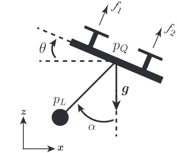
Fig. 1. 2D UAV model with a cable suspended load.f1andf2are the forces

generated by the two propellers.pQis a vector representing the position of the UAV andpLthe position of the load.θis the pitch angle with respect to the horizontal position.αis the angle of the load with respect to the z-axis andgis the gravity constant

In Fig. 1 a sketch is shown of the UAV with cable suspended load that need to be modelled and controlled. The center of mass position of the quadrotor and load can be described in

inertial frame withpQ= [x, z]T ∈R2 the quadrotor position

and pL = [xL, zL]T ∈ R2 the position of the load. The

attitude is described by θ ∈Rwith respect to the horizontal

position. The rotation of the load with the z-axis is described

byα∈R. The UAV is actuated by two propellers generating

the forcesf1andf2∈R≥0. The assumption is that the cable

formalism the dynamics of the UAV and load are obtained [5],i.e,

(M+m)(¨z+g) +mL(cosαα˙2+ sinαα¨) =u1cosθ (1a)

(M+m)¨x+mL(sinαα˙2−cosαα¨) =u1sinθ (1b)

mL2α¨+mLsinαz¨−mLcosαx¨+mgLsinα= 0 (1c)

Jθ¨=u2 (1d)

Where:

• M, m: are the mass of quadrotor and load, respectively

• u1=f1+f2: is the total thrust generated by the propellers

• L: is the length of the cable

• J: is the inertia of the quadrotor

• u2 = (f1−f2)b: is the moment due to the propellers

where b is the distance between the center of mass and

the motors.

III. CONTROLDESIGN

In this section the passivity based control design of the system is presented and the stability is analysed by using Lyapunov theory. The goal of the controller is to move from point to point while the swing in the load stay bounded near the equilibrium.

A. Passivity Based Control

The idea behind passivity based control is that each subsys-tem consist of an certain energy. By adding these energies together the energy of the overall system is obtained. By controlling this energy such that the used energy is minimized a stabilized system can be obtained [8]. Due to the passivity property there will be no more energy stored then that is supplied to the system.

B. Control of a quadrotor UAV with a cable suspended load

˙ α Lateral+Load Controller Attitude Controller Attitude Dynamics Lateral+Load Dynamics

θD θ

x x d z z d u2 Vertical Controller Vertical Dynamics u1 ˙ α ˙ α ˙ α α α α α α¨

¨ α

¨ α u1

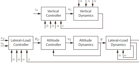
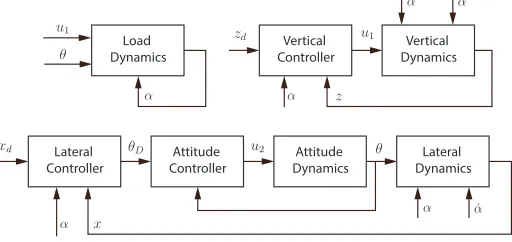
Fig. 2. Control architecture of the UAV with the cable suspended load

To control the UAV with the cable suspended load the control architecture as described in Fig. 2 is used. It can be seen that a fast high gain attitude controller is used such that

θ ≈ θD where θD is the desired pitch angle. Furthermore

is assumed that during movement the UAV stays near the

hovering position: This means thatθD≈0, and therefore that

cosθD≈1andsinθD≈θD. From Fig. 2 it can also be seen

that the lateral and load dynamics are taken together. This is because both dynamics are coupled with each other (1b),(1c).

Within this controller can be assumed that ¨z→0 because the

vertical position is assumed to be at a constant altitude during movement to a desired location. This controller is controlling

αto zero and xtoxd. With this the reduced load dynamics

is obtained:

lim

α→0α¨=

1

Lx¨ (2)

The vertical dynamics are affected by the load dynamics and

the controller is controlling z to zd with the input u1. The

control inputsu1 andθD should be designed such that:

¨

z=−k_pz(z−zd)−kzdz˙ (3)

¨

x+ ¨α=−k_px(x−xd+α)−kdx( ˙x+ ˙α) (4)

This is obtained by choosing the inputs as:

u1= (M+m)(uz+g) (5)

θD=

M L+mLsin2α u1(L+ cosα) (−k

x

p(x−xd+α)

−kxd( ˙x+ ˙α) +

mLsinα(L+ cosα)

M L+mLsin2α α˙ 2

−(M+m)(M+m+mLcosα)

M L+mLsin2α ) (6)

This can be proofed by the following. When considering the hovering position the vertical dynamics can be approximated by [9]:

¨

z=uz+dz (7)

withuz the input to the system and dz an exogenous

distur-bance. From this, uz can be described by the following to

obtain PD dynamics in the vertical dynamics.

uz=−kpz(z−zd)−kzdz˙+

mL

M+m(cosαα˙

2_{+ sinαα¨)}

(8)

The combined dynamics of x and αneed to be described

with the following equation to also obtain PD dynamics.

¨

x+ ¨α= u1(L+ cosα)

M L+mLsin2αθD

−mLsinα(L+ cosα)

M L+mLsin2α α˙ 2

−(M +m)(M +m+mLcosα)

M L+mLsin2α (9)

C. Lyapunov Stability

To see if the designed controller will result in a stable system a proof of stability is performed by using a Lyapunov function [10]. For this system, the following candidate Lya-punov function is chosen:

V = 1

2( ˙x+ ˙α)

2

+1 2z˙

2

+1 2k

x

p(x−xd+α)2

+1 2k

z

p(z−zd)2 (10)

The following is obtained when this function is differentiated.

˙

V = ( ˙x+ ˙α)(¨x+ ¨α) + ˙zz¨

+kx_p(x−xd+α)( ˙x+ ˙α) +kzp(z−zd) ˙z (11)

1 2( ˙. . .)

2_{denotes the kinetic energy and}1

2k

β

p(. . .)2the potential

8

0 5 10 15 20 25 30 35 40

position [m]

0 0.1 0.2 0.3 0.4 0.5 0.6

Position of UAV

X Z

0 5 10 15 20

angle [degree] 0 0.2 0.4

Angle made by load

α

time [s]

0 5 10 15 20

angle [degree]

0 0.2 0.4

Pitch of UAV

θ

Fig. 3. Position response of the system if a setpoint of 0.5 is given in x and z. The second plot shows that the load stabilises after this position change. The pitch angle of the UAV stays near zero.

lateral and vertical dynamics are included, which results in cancelling out some terms.

˙

V = −kx_d( ˙x+ ˙α)2−kz_dz˙2≤0 (12) This result shows that the Lyapunov function is negative

semi-definite which means thatxdandzdare stable setpoints. With

this derivation, stability is guaranteed for the lateral, vertical and load dynamics. Using LaSalle’s Theorem asymptotically stability is shown.

IV. SIMULATIONS

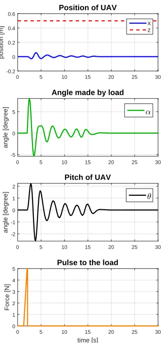
This section discusses the results obtained via simulations. To validate the designed controller two simulations in 20sim [11], a modelling and simulation program, are performed. In the first experiment a setpoint in x and z of 0.5m is given to validate the setpoint response of the proposed controller. The gains are chosen such that the resulting swing is bounded and that the setpoint response is smooth without an overshoot. The result of this simulation is shown in Fig. 3. It can be noticed that the setpoint is reached smoothly without an overshoot. In the load angle part can be seen that the angle is kept bounded

during movement. The same holds for the pitch angleθ.

In the second test a hovering position is kept and a distur-bance is given to load. In this way the behaviour can be seen of how the system responses to a large swing in the load. The result of this simulation is shown in Fig. 4. To compensate for the swing in the load a small disturbance can be observed in the x position of the UAV. The plot shows also that the angle in the load is reduced quickly and that the pitch angle

θ stays near zero. It also show that the UAV is counteracting

the swing by moving in the other directions.

0 5 10 15 20 25

position [m]

-0.2 0 0.2 0.4

0.6 Position of UAV

X Z

0 5 10 15 20 25

angle [degree]

-5 0 5

Angle made by load

α

0 5 10 15 20 25

angle [degree]

-2 0 2

Pitch of UAV

θ

time [s]

0 5 10 15 20 25

Force [N]

0 1 2 3 4 5

Pulse to the load

Fig. 4. Result when a disturbance after 2 seconds is given to the load. To compensate for the swing the UAV need to change his x-position. The angle with the load is asymptotically going to his equilibrium due to the counteracting of the UAV.

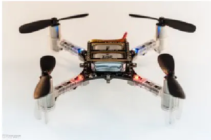
Fig. 6. The CrazyFlie 2.0 [12]

V. EXPERIMENTS

CrazyFlie 2.0

Load

Setup Ground Station

Testing Area

Attitude Control

Cable

Spheres with reflective tape

Communication

Pose Estimation

ˆ

x= ( ˆx , y ,ˆ z ,ˆ φ ,ˆ θ ,ˆ ˆγ)

NaturalPoint Tracking Tools

Data Exchange

Marker Data Pose

Control Inputs

Optitrack Area Quadrotor

+ Setpoint-Load

Control

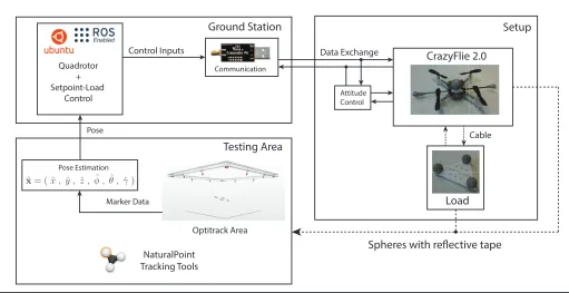
Fig. 5. System Overview: the overall system consisting of one CrazyFlie 2.0 to which a load is connected. The setup to which reflective markers are attached is placed in an optitrack area. A motion tracking system is used to detect the trackable position from which the absolute pose is estimated. The ground station is used to communicate with the UAV via a radio link and to run the setpoint and load controller. Over this radio link the control inputs can be send. The robotic operating system (ROS) is used on ubuntu to communicate between the different software modules and the Crazyflie.

measured. The maximum recommended amount of payload to be carried is limited to 15g [15]. In this experiment a payload of 12.4g is used. This is the combination of 8.6 g load and 3.8 g for the optitrack markers and the carbon tube to attach the reflective markers on. For the cable a length of 1m is taken which is 95cm after attaching to the Crazyflie.

The Crazyflie itself is controlled via an internal attitude controller and a thrust for the vertical direction. Via ROS only a velocity can be sent as an input for the lateral direction to the UAV. For this it is assumed that for small angle changes it can be considered as setting a velocity. For the error the difference is taken between the current position and desired position. To obtain the velocity and acceleration of the angle a state variable filter is used based on a butterworth low pass filter [16]. To obtain the acceleration a third order filter is needed. The transfer function of this filter is as follows:

H(s) = ω

3

c

s3_{+ 2ω}

cs2+ 2ω2c+ωc3

(13)

Whereωcis the desired cut-off frequency. By using this filter a

phase shift is introduced in the outputs. By increasing the cut-off frequency this shift is lowered but more noise is allowed on the outputs. For this a consideration need to be made on how much noise or delay is allowed. For this experiment a cut-off frequency of 1.5Hz is taken. With this a phase delay of 0.3 seconds is introduced.

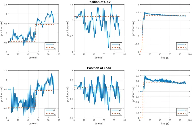
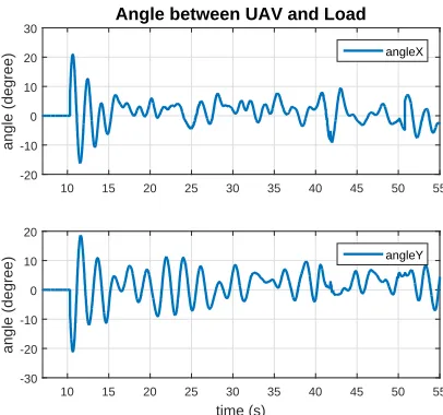
In Fig. 8 the result of the experiment with the UAV and load can be seen. It can be noticed that controller is able to make a stable flight but that the position of the UAV does

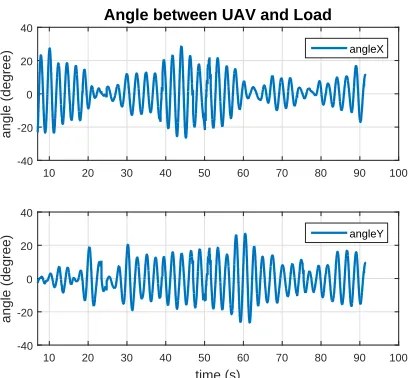
not converge to the desired setpoint. The swing of the load is

kept to a minimum of 28◦ in the x-direction and 27◦ in the

y-direction. This can be seen in Fig. 7. In the x-direction it has a setpoint error of 72cm and in the y-direction of 98cm. From Fig. 9 can be concluded that the assumption that the pitch and roll are small during control is achieved since they stay

within 10◦for the biggest part of the experiment. To see if the

controller it self is stable an experiment is performed where

no load is attached and the angleαis set to zero. In Fig. 10

the result of this experiment is shown. This plot shows that the UAV itself is able to stay in his desired position but that the load adds to much disturbance to achieve a stable system. A big offset can be noticed in the vertical direction due to the fact that the controller still compensates for the mass of the load with his initial thrust offset.

A. Discussion on experiments

10

time (s)

0 20 40 60 80 100

postion x (m)

-1 -0.5 0 0.5 1 1.5 x xd time (s)

0 20 40 60 80 100

postion y (m)

-1 -0.5 0 0.5

Position of UAV

y

yd

time (s)

0 20 40 60 80 100

postion z (m)

-1 -0.5 0 0.5 1 1.5 2 z zd time (s)

0 20 40 60 80 100

postion x (m)

-1 -0.5 0 0.5 1 1.5 xL xd time (s)

0 20 40 60 80 100

postion y (m)

-1.5 -1 -0.5 0 0.5 1

Position of Load

yL

yd

time (s)

0 20 40 60 80 100

postion z (m)

-1 -0.8 -0.6 -0.4 -0.2 0 0.2 0.4 0.6 0.8 zL zd

Fig. 8. Recorded Position of UAV and load during experiment. Setpoint z is -1 at the start to guarantee that the UAV stays one the ground when the communication between the UAV and PC is started.

time (s)

0 20 40 60 80 100

pitch (degree) -15 -10 -5 0 5 10 15 20 25 pitch time (s)

0 20 40 60 80 100

roll (degree) -15 -10 -5 0 5 10

15 Attitude of UAV

roll

time (s)

0 20 40 60 80 100

yaw (degree) -8 -6 -4 -2 0 2 4 6 8 yaw

Fig. 9. Measured attitude of UAV during experiment.

time (s)

0 20 40 60 80 100

postion x (m)

-0.4 -0.2 0 0.2 0.4 0.6 0.8 x xd time (s)

0 20 40 60 80 100

postion y (m)

-0.25 -0.2 -0.15 -0.1 -0.05 0 0.05 0.1

Position of UAV

y

yd

time (s)

0 20 40 60 80 100

postion z (m)

-1 -0.5 0 0.5 1 1.5 z zd time (s)

0 20 40 60 80 100

pitch (degree) -15 -10 -5 0 5 10 15 20 pitch time (s)

0 20 40 60 80 100

roll (degree) -10 -5 0 5 10 15

Attitude of UAV

roll

time (s)

0 20 40 60 80 100

yaw (degree) -8 -6 -4 -2 0 2 4 6 8 yaw

10 20 30 40 50 60 70 80 90 100

angle (degree)

-40 -20 0 20 40

Angle between UAV and Load

angleX

time (s)

10 20 30 40 50 60 70 80 90 100

angle (degree)

-40 -20 0 20 40

angleY

Fig. 7. Angle between the load and the UAV during the experiment. The plot starts at 7 seconds since on that moment the load controller is enabled. Further it shows that the angles stay bounded overtime

errors in the lateral directions when carrying a load. Since most of this thrust is already needed to stay in his vertical position. Also due to the small size of the Crazyflie the life time of the battery is not long and by this a recharge is needed after a couple of minutes flight time.This decay goes more rapidly when a load is attached. Also the controller performance starts to decrease when the battery is discharging. Taking the rope length to small will cause that the load is pushed away to much by the thrust of the UAV which is exerting a moment on the UAV which is also influencing the position of the UAV.

VI. CONCLUSIONS& RECOMMENDATIONS

A. Conclusion

In this work, a passivity based controller has been designed such that minimum swing is achieved in the load. Both controllers in simulation are performing as expected and can control the system to a desired setpoint with ensuring minimal swing. During experiment the UAV is able to damp out most of the swing after lift off. The system is also holding this bounded swing overtime but the system is not able to stabilize his position around the desired position. By not using the load and

settingαto zero the load controller is able to stabilize around

the desired position. Extensive controller tuning is performed to improve the setpoint response but without better results.

B. Recommendations for future work

In this project the controller is designed in a 2D space but tested in 3D space. Therefore to improve the controller it is recommended to model and design the controller in 3D space. To achieve better simulation Since the Crazyflie 2.0 are not performing well while carrying a load due to there limit payload and low weight it will be a good experiment to see how this kind of controller performs on a slightly bigger quadrotor. In this way the load will probably not be affected by the thrust to much. Also designing a separate controller for the pitch and roll direction can improve the performance.

Extending the Gazebo model such that a load can be added to the UAV is also recommended since then more accurate simulation can be performed. Extend work by using multiple drones is also recommended since in this way the advantages of small drones is utilized.

REFERENCES

[1] L. Marconi, R. Naldi, A. Torre, J. Nikolic, C. Huerzeler, G. Caprari, E. Zwicker, B. Siciliano, V. Lippiello, R. Carloni, and S. Stramigioli, “Aerial service robots: An overview of the AIRobots activity,” in

Proceedings of IEEE International Conference on Applied Robotics for the Power Industry, 2012, pp. 76–77.

[2] L. Marconi, C. Melchiorri, M. Beetz, D. Pangercic, R. Siegwart, S. Leutenegger, R. Carloni, S. Stramigioli, H. Bruyninckx, P. Do-herty, A. Kleiner, V. Lippiello, A. Finzi, B. Siciliano, A. Sala, and N. Tomatis, “The SHERPA project: Smart collaboration between humans and ground-aerial robots for improving rescuing activities in alpine environments,” in Proceedings of IEEE International Symposium on Safety, Security, and Rescue Robotics, 2012, pp. 1–4.

[3] G. Gioioso, A. Franchi, G. Salvietti, S. Scheggi, and D. Prattichizzo, “The flying hand: A formation of uavs for cooperative aerial tele-manipulation,” in Proceedings of IEEE International Conference on Robotics and Automation, 2014, pp. 4335–4341.

[4] K. Sreenath and V. Kumar, “Dynamics, control and planning for co-operative manipulation of payloads suspended by cables from multiple quadrotor robots,” inRobotics: Science and Systems (RSS), 2013. [5] M. Nicotra, E. Garone, R. Naldi, and L. Marconi, “Nested saturation

control of an uav carrying a suspended load,” in Proceedings of American Control Conference, June 2014, pp. 3585–3590.

[6] K. Sreenath, T. Lee, and V. Kumar, “Geometric control and differential flatness of a quadrotor uav with a cable-suspended load,” inProceeding of IEEE 52nd Annual Conference on Decision and Control, 2013, pp. 2269–2274.

[7] T. Lee, “Geometric control of multiple quadrotor uavs transporting a cable-suspended rigid body,” in Proceedings of IEEE 53rd Annual Conference on Decision and Control, 2014.

[8] R. Ortega, A. Van der Schaft, I. Mareels, and B. Maschke, “Putting energy back in control,”IEEE,Control Systems, vol. 21, no. 2, pp. 18– 33, 2001.

[9] M. Fumagalli, R. Naldi, A. Macchelli, F. Forte, A. Keemink, S. Strami-gioli, R. Carloni, and L. Marconi, “Developing an aerial manipulator prototype: Physical interaction with the environment,” IEEE,Robotics Automation Magazine, vol. 21, no. 3, pp. 41–50, 2014.

[10] H. Khalil, Nonlinear Systems, ser. Pearson Education. Prentice Hall, 2002. [Online]. Available: https://books.google.nl/books?id=t d1QgAACAAJ

[11] Controllab Products, “20-sim: The power in moddeling.” [Online]. Available: http://www.20-sim.com/

[12] Bitcraze. (2015) The Crazyflie 2.0. [Online]. Available: https: //www.bitcraze.io/crazyflie-2/

[13] ROS, “ROS: An open-source Robot Operating System.” [Online]. Available: http://www.ros.org/about-ros/

[14] Naturalpoint, Inc, “Optical Tracking Solutions, optitrack: motion caputre systems. Version 2.3.3.” [Online]. Available: http://www.optitrack.com/ [15] Bitcraze Wiki. (2015) Crazyflie 2.0 hardware specification. [Online]. Available: https://wiki.bitcraze.io/projects:crazyflie2:hardware: specification

[16] Butterworth, S, “On the Theory of Filter Amplifiers,” October 1930. [Online]. Available: http://www.gonascent.com/papers/butter.pdf [17] M. de Roo, “Optimal Event Handeling By a UAV Network,” Master’s

12

APPENDIXA

CONTROLDESIGN WITHSYSTEMDECOUPLING

To obtain a passivity based controller with system decou-pling the system should first be decoupled [5]. Due to this the system can be divided in two loops: The inner loop and outer loop. The inner loop will control the attitude of UAV by using

the input u2. With the inputs u1 andθthe outer loop will be

controlled. With this is assumed that the vertical dynamics are not influenced by the lateral and load dynamics and controller

byu1. These will be controlled by the desired pitch angleθD.

For this the attitude controller will be designed fast such that

θ ≈ θD . In Fig. 11 the control architecture can be seen to

achieve this goal [9]. The symbolsxd andzd are the desired

positions of the UAV.αis the angle between the UAV and the

load. ˙ α Lateral Controller Load Dynamics Attitude Controller Attitude Dynamics Lateral Dynamics θ θ θ D x x d z z d u2 Vertical Controller Vertical Dynamics u1 u1 ˙ α

Fig. 11. Control architecture of the 1 UAV with the cable suspended load

The goal of this controller is to choose the controlling input

u1andθDsuch that the resulting system is able to move stably

from point to point and meanwhile bound the swing in the load near his equilibrium.

During the derivation of the controller the trigonometric identi-ties in 14 and 15 will be used. For this is assumed that the UAV stays near his hovering position during his flight. With small

θD it can be approximated that cosθD≈1 andsinθD≈θD.

with this:

cos(θ−2α) = cosθcos 2α+ sinθsin 2α (14)

= cos 2α+θDsin 2α

sin(θ−2α) = sinθcos 2α−cosθsin 2α (15)

=θDcos 2α−sin 2α

In (16) the derivation is shown of the dynamics in the z-direction. For simplification (14) is used.

¨

z= −g− m

M+mLcosαα˙

2₊ 1

M +m(cosθ

+ m

2M(cosθ−cos(θ−2α)))u1 (16a)

= −g− m

M+mLcosαα˙ 2

+ 1

M+m(1 + m

2M(1−cos 2α−θdsin 2α))u1 (16b)

= −g+ u1

M+m+

u1m

2M(M+m)(1−cos 2α−θDsin 2α)

− m

M +mLcosαα˙

2 _(16c)

With (15) the lateral dynamics in (17) are simplified.

¨

x= − m

M +mLsinαα˙

2₊ 1

M +m(sinθ

+ m

2M(sinθ−sin(θ−2α)))u1 (17a)

= − m

M +mLsinαα˙

2₊ 1

M +m(θD

+ m

2M(θD−θDcos 2α−sin 2α))u1 (17b)

=gθD+

gm

2M(θD−θDcos 2α)

− m

M +mLsinαα˙ 2

− gm

2Msin 2α (17c)

By definingAandB as follows the z and x dynamics can

be simplified:

A= (1 + m

2M(1−cosα−θDsin 2α)) (18) B= (g+ gm

2M(1−cos 2α)) (19)

This results in the following dynamics for ¨xandz¨:

¨

z=−g− m

M +mLcosαα˙

2₊ 1

M+mAu1 (20a)

¨

x=BθD−

m

M+mLsinαα˙

2₋ gm

2M sin 2α (20b)

The resulting dynamics can be approximated by (21) when assuming the hovering position of the UAV [9].

¨

γ=uγ+dγ with γ∈[z, x] (21)

Hereuγ is the control input to the system anddγ exogenous

disturbances. Leaving out the disturbances, the inputsu1 and

θD are chosen as:

u1=

(uz+g)(M+m)

1 + m

2M(1−cos 2α−θDsin 2α)

(22)

θD=

ux

g+₂gm_M(1−cos 2α) (23)

To obtain a PD-controller the control inputsuz and ux need

to be chosen as in (24a).

uz=−kpz(z−zd)−kdzz˙+

m

M +mLcosαα˙

2 _(24a)

ux=−kpx(x−xd)−kdxx˙+

m

M+mLsinαα˙

2₋ gm

2M sin 2α

(24b)

When the inputsu1andθD are in included in (20) they result

in the following PD dynamics:

¨

z=−kz_p(z−zd)−kzdz˙ (25a)

¨

0 5 10 15 20 25 30 position [m] 0 0.1 0.2 0.3 0.4 0.5 0.6

Position of UAV

X Z

0 5 10 15 20 25 30

angle [degree]-1 0 1

Angle made by load

α

time [s]

0 5 10 15 20 25 30

angle [degree]

-0.5 0 0.5 1

Pitch of UAV

θ

Fig. 12. Simulation result of a UAV with a cable suspended load

A. Lyapunov Analysis

A Lyapunov function will be used to check stability of the position. The Lyapunov function in (26a) is used for this case.

1 2γ˙

2_{denotes the kinetic energy and} 1

2k

γ

p(γ−γd)2the potential

energy of the system. Taking the derivative, results in (26d).

V = 1

2x˙

2₊1

2z˙

2₊1

2k

x

p(x−xd)2+

1 2k

z

p(z−zd)2 (26a)

˙

V = ˙xx¨+ ˙zz¨+k_px(x−xd) ˙x+kzp(z−zd) ˙z (26b)

= −kx_p(x−xd) ˙x−kdxx˙

2_+kx

p(x−xd) ˙x

−kzp(z−zd) ˙z−kdzz˙

2

+kzp(z−zd) ˙z (26c)

˙

V = −kxdx˙

2

−kdzz˙

2

≤0 (26d)

This result shows that the derivative is negative semi-definite and by this the system is stable for his position. Since stability for the load dynamics can not be guaranteed with a Lyapunov function it can not be said that the whole system is stable as well. With this derivation, stability is guaranteed for the lateral and vertical dynamics. Now only the load angle dynamic need to be checked for stability but this is the most difficult part to do since there is no direct control on these dynamics.

B. Simulations

In Fig. 12 and Fig. 13 the simulation results can be observed of the designed controller. These simulations are performed in 20sim. One simulation is done when a setpoint of 0.5 is given in the x- and z-direction. In the other simulation a pulse is given to the load to see if the UAV is still able to damp out the caused swing. In both cases a small disturbance can be noticed in the x-position to counteract the swing in the load.

Furthermore can be seen that the angleαandθ stay bounded

overtime.

0 5 10 15 20 25 30

position [m]

-0.2 0 0.2 0.4

0.6 Position of UAV

X Z

0 5 10 15 20 25 30

angle [degree]

-5 0 5

Angle made by load

α

0 5 10 15 20 25 30

angle [degree]_-2 -1 0 1 2

Pitch of UAV

θ

time [s]

0 5 10 15 20 25 30

Force [N] 0 1 2 3 4 5

Pulse to the load

Fig. 13. Simulation result of a UAV with a cable suspended load when a pulse is added to the load

C. Experiments

The controller is also tested in an optitrack environment with a real setup. The same setup as in the main paper is used to perform this experiment. In Fig. 8 the position results can be seen. It can be noticed that the system is not able to go to the desired setpoint. Especially in the y-direction. Here it is drifting from the desired position. The vertical position is not reached due to probably the attached load and that the minimal offset thrust to compensate for gravity is set to low. The resulting load angles are shown in Fig. 14. It shows that

the controller is able to bound the load angle within 10◦.

Fig. 16 shows that the attitude stays small during movement of the UAV.

D. Conclusion

14

10 15 20 25 30 35 40 45 50 55

angle (degree) -20 -10 0 10 20 30

Angle between UAV and Load

angleX

time (s)

10 15 20 25 30 35 40 45 50 55

angle (degree) -30 -20 -10 0 10 20 angleY

Fig. 14. Resulting angle between UAV and load during the experiment. Plot stays zero until 10 seconds since on that moment the load controller is enabled.

time (s)

0 10 20 30 40 50

postion x (m)

-1.5 -1 -0.5 0 0.5 1 x x_d time (s)

0 10 20 30 40 50

postion y (m)

-0.4 -0.2 0 0.2 0.4 0.6 0.8

Position of UAV

y

yd

time (s)

0 10 20 30 40 50

postion z (m)

-1 -0.5 0 0.5 1 1.5 z zd time (s)

0 10 20 30 40 50

postion x (m)

-1.5 -1 -0.5 0 0.5 1 xL time (s)

0 10 20 30 40 50

postion y (m)

-0.5 0 0.5 1

Position of Load

yL

time (s)

0 10 20 30 40 50

postion z (m)

0 0.1 0.2 0.3 0.4 0.5 zL

Fig. 15. Recorded Position of UAV and load during experiment. Setpoint z is -1 at the start to guarantee that the UAV stays one the ground when the communication between the UAV and PC is started. The minimal thrust offset to compensate for gravity was set to low to reach the desired altitude.

time (s)

0 10 20 30 40 50

pitch (degree) -20 -15 -10 -5 0 5 10 pitch time (s)

0 10 20 30 40 50

roll (degree) -8 -6 -4 -2 0 2 4 6 8

Attitude of UAV

roll

time (s)

0 10 20 30 40 50

yaw (degree) -10 -8 -6 -4 -2 0 2 4 6 8 10 yaw

APPENDIXB MANUAL

In this appendix the use of the software package will be explained in chronological order. The package is available through the Robotics and Mechatronics group of the University of Twente. The manual is based on the manual written in [17] with some additions and clarifications.

A. Prerequisites

The software package is written for ROS. At the date that this package is developed the current version was ROS indigo. Ubuntu 14.04 is used as operating system to run ROS. The following prerequisites are assumed for this manual:

1) Ubuntu 14.04 or any derivative based on this (Xubuntu 14.04, Lubuntu 14.04, etc).

2) ROS Indigo installation according to http://wiki.ros.org/ indigo/Installation/Ubuntu with a Desktop-Full Install.

3) Crazyflie client (https://github.com/bitcraze/

crazyflieclients-python) 4) clean catkin workspace

5) Knowledge on how to use Optitrack

B. Installation

The ram crazy package requires three external packages:

• hector quadrotor: http://wiki.ros.org/hectorquadrotor

• crazyflie ros: http://wiki.ros.org/crazyflie

• mocap optitrack: http://wiki.ros.org/mocapoptitrack

Thehector quadrotorpackage is used to simulate a quadrotor

in gazebo. To connect to the crazyflie thecrazyflie rospackage

is used. The data obtained from the optitrack system need to

be translated to a ROS message. This is handled in the

mo-cap optitrackpackage. The current versions of these packages

are included by theram crazysuch that compatible issues are

prevented. But using the current version might be interesting since more and updated options might be available. After unpacking the packages in the catkin workspace, execute the following commands in a terminal to solve the dependencies.

$ cd ˜ / p a t h t o c a t k i n w o r k s p a c e

$ r o s d e p i n s t a l l −−from−p a t h

s r c −−i g n o r e−s r c

This will install all the required packages, the installation wiil request confirmation of installing the packages serval times. Run the following command inside you workspace through a terminal to compile the catkin workspace.

$ c a t k i n m a k e

To compile the package completely it might be necessary to to run this command several times.

C. Usage of package

Before the package can be used make sure that the following is done to make everything work properly. In Ubuntu all the python .py files need to be an executable before they work. To do this run the following commands for all the python files:

$ cd ˜ / c a t k i n w o r k s p a c e / s r c / r a m c r a z y / py $ s u d o chmod +x f i l e n a m e . py

Also make sure that the following lines are included in bottom

of the/.bashrcfile. Since otherwise this command need always

be executed after opening a new terminal. To acces this file execute the following command and paste the two lines.

$ g e d i t ˜ / . b a s h r c

s o u r c e / o p t / r o s / i n d i g o / s e t u p . b a s h

s o u r c e ˜ / c a t k i n w s / d e v e l / s e t u p . b a s h

By placing these lines in the /.bashrc they will be executed

automatically after opening a new terminal.

Now everything should be set to start using this package. There are two launch file available. One which starts only

theinterface.pyscript and one which starts this script and the

gazebo program Gazebo. For only launching the interface.py

script execute the following (tab can be used to auto complete):

$ r o s l a u n c h r a m c r a z y

i n t e r f a c e l a u n c h . l a u n c h

After this gazebo can be started separately with the following command:

$ r o s l a u n c h r a m c r a z y

q u a d r o t o r e m p t y w o r l d . l a u n c h

Executing the following command will do both at once:

$ r o s l a u n c h r a m c r a z y

r a m c r a z y e m p t y w o r l d . l a u n c h

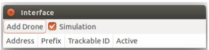
In Fig. 17 the interface is shown after start-up. With the

Simulation toggle button can be specified if the test is

performed in simulation or in experiment. Depending on the selection, ROS will start-up different publishers and

subscribers. Four columns can also be noticed. The Address

column displays the radio address that is used to connect to that drone. The first value shows the radio ID, the second the drone ID and the last one show the used bandwidth for communication. The second column displays the prefix of the drone used by ROS to distinguish each drone during control. In the optitrack environment each drone need to given an ID.

This one is specified by theTrackable ID column. The value

present here need to be given to the trackable in optitrack. The last column shows if the controller for that drone is active. This allows to send the pose from optitrack to ROS.

With the Add Drone button an arbitrary number of drones

can be added. The increment is set to 60 but can be changed. The Load has been given the trackable ID of 12. After adding one drone the interface will look like as in Fig. 18. To make the controller active double click that row. This will start-up the controller shown in Fig. 19. This interface has different buttons and these are explained below. Moving the sliders will change the values. Changing the setpoint sliders and offset thrust slider will directly change the controller. After

changing the sliders in the gain section theSet Gains button

16

Take-off:

gets the current position and sets the z-setpoint to one.

Land:

Lands the UAV.

Get Setpoint:

Changes the setpoints of the interface to the current position measured by optitrack.

Go to setpoint:

adds a value to the current position and makes this a new setpoint.

Toggle Radio:

Activates the communication with the drone

Spawn Simulation

Spawns the drone in Gazebo

Save Data:

Saves the data to a specified location. default location is /.ros/ folder. In the .cpp file of the controller the location and what need to be saved can be set.

Publish Setpoint:

Enables the publishing of the setpoint.

Lissajous test:

Starts the path following of a Lissajous figure.

Setpoint drone0:

Uses the setpoint of drone0 with an distance in the x-direction specified by the slider next to it. Used for load transport with 2 UAVs.

1/2 Drone(s):

Specifies with how many drones the load transporta-tion is performed.

Enable Load Control:

Enables the load control part and also sets the gains to be used.

Get Current:

Allows the current I-action to be read and sent to the interface, in this way the offset can be determined using the I-action of the PID controller.

Set Gains Control Without Load:

Sets the default gains for controlling without load.

Set Gains Control With Load:

Sets the default gains for controlling with load. Gains are restored depending on which toggle is active of the one or two drones.

Set Gains:

Sets the gains depending on how the sliders are set. In Fig. 20 an example of gazebo is shown when two drones are used. RViz can be used to visualize the current setpoint and pose of the UAV. It can be launched by executing the following command:

$ r o s l a u n c h r a m c r a z y

r v i z r a m l a u n c h . l a u n c h number : = T r a c k a b l e I D

In Fig. 21 the result of this command is shown. In this case also the Lissajous path is enabled and by this also shown in RViz. The two arrows display the orientation of the UAV and the velocity vector.

Fig. 17. Interface after starting up the interface.py script

Fig. 18. Example of the interface with two drones added

Fig. 19. Controller interface to fly with the crazyflie. In this interface the control parameters can be changed and the desired setpoint can be given. It is also possible to enable the control to fly with a load.

D. How to fly with the load

The following can be done to be able to fly with a cable suspended load.

• place the drone and load in the optitrack area such that

the load is along the x- or y-axis.

• start-up the interface and the controller for drone0

• PressGet Setpoint

• Enable 1 Drone

• PressSet Gains Control without Load

• Enable Toggle Radio,Publish Setpoint will enable

auto-matically

• Slide the slider ofSetpoint Zcarrefully up until the drone

and load are of the ground

Fig. 20. Gazebo after two drones are added