University of Warwick institutional repository: http://go.warwick.ac.uk/wrap
This paper is made available online in accordance with
publisher policies. Please scroll down to view the document
itself. Please refer to the repository record for this item and our
policy information available from the repository home page for
further information.
To see the final version of this paper please visit the publisher’s website
.
Access to the published version may require a subscription.
Author(s): RG Cowell, P Thwaites and JQ Smith
Article Title: Decision making with decision event graphs
Year of publication: 2010
Link to published article:
http://www2.warwick.ac.uk/fac/sci/statistics/crism/research/2010/paper
10-15
Robert G. Cowell
Faculty of Actuarial Science and Insurance, Cass Business School, City University, London, 106 Bunhill Row, London EC1Y 8TZ, UK, [email protected]
Peter Thwaites, James Q. Smith
Statistics Department, University of Warwick, Coventry CV4 7AL, UK, [email protected] [email protected]
We introduce a new modelling representation, the Decision Event Graph (DEG), for
asym-metric multistage decision problems. The DEG explicitly encodes conditional independences
and has additional significant advantages over other representations of asymmetric decision
problems. The colouring of edges makes it possible to identify conditional independences on
decision trees, and these coloured trees serve as a basis for the construction of the DEG.
We provide an efficient backward-induction algorithm for finding optimal decision rules on
DEGs, and work through an example showing the efficacy of these graphs. Simplifications of
the topology of a DEG admit analogues to the sufficiency principle and barren node deletion
steps used with influence diagrams.
Key words: Asymmetric decision problem; Backwards induction; Decision tree; Extensive form; Influence diagram; Local computation; Optimal policy.
1.
Introduction
The decision tree is one of the oldest representations of a decision problem (Raiffa 1968, Lindley 1985, Smith and Thwaites 2008a). It is flexible and expressive enough to represent asymmetries within both the decision space and outcome space, doing this through the topological structure of the tree. The topology of the tree can also be used to encode the natural ordering, or unfolding, of decisions and events. By exploiting the topology optimal decision rules may be found using backward induction.
paper is to introduce a new graphical representation of multistage decision problems together with a local computation scheme over the graph for finding optimal decision policies. This new represen-tation we call theDecision Event Graph (DEG). This compact representation is particularly suited to decision problems whose state spaces do not admit a product form. As well as representing a decision problem, the DEG also provides a framework for computing decision rules. As the DEG has fewer edges and nodes than a decision tree, the computation of such rules is necessarily more efficient using this new graph. In addition, unlike the standard decision tree, the DEG allows for the explicit depiction of conditional independence relationships.
A variety of alternative graphical representations have been developed to alleviate the complexity associated with decision trees, and allow for local computation. The most commonly used and influ-ential of these is theinfluence diagram(ID) (Howard and Matheson 1984, Olmsted 1983, Shachter 1986, Jensen and Nielsen 2007, Smith and Thwaites 2008b, Howard and Matheson 2005, Boutilier 2005, Pearl 2005). Modifications to ID solution techniques have been made since their introduction in, for example, (Smith 1989a, Cowell 1994, Jensen et al. 1994). The principal drawback of the ID representation is that it is not suited to asymmetric decision problems where different actions can result in different choices in the future (Covaliu and Oliver 1995) or different events give rise to very different unfoldings of the future. Attempts have been made (Smith and Matheson 1993) to adapt IDs for use with such problems, and Call and Miller (1990) developed techniques which used both decision trees and IDs. The Sequential Decision Diagram, a representation similar to an ID but with context-specific information added to the edges, was introduced by Covaliu and Oliver (1995), and Shenoy (1996) proposed the Valuation Network. A good discussion of the pros and cons of the various techniques for tackling asymmetric problems is given by Bielza and Shenoy (1999).
on a secondary structure such as a junction tree (Cowell et al. 1999, Jensen and Nielsen 2007) or by modifying the ID with arc reversal and barren node removal operations (Shachter 1986). These factors both increase computational complexity and hinder interpretation.
In contrast the DEG introduced in this paper, by explicitly retaining the asymmetries, does not require additional dummy states or values, giving a more streamlined specification. Furthermore when using a DEG no secondary structures need be created, and the DEG can be used directly as a framework on which to calculate an optimal policy rapidly.
In this paper we concentrate of the relationship between DEGs and their corresponding decision trees. DEGs are closely related toChain Event Graphs (CEGs) (Smith and Anderson 2008), which are themselves functions of event trees (or probability trees). Indeed, if a DEG consists solely of chance nodes, (so that is it has neither utility nor decision nodes), and if the edges only have probabilities associated with them, then the DEG reduces to a CEG.
A DEG is a function of a decision tree, although it is not necessary in all problems to first construct a decision tree before creating the DEG. There are a number of different types of decision tree, dependent on the method of construction. Commonly used types includeExtensive form(EF),
Normal form and Causal trees (Smith and Thwaites (2008a)). But regardless of type, all trees consist of a root node from which directed paths emanate consisting of edges and vertices, each path terminating in a leaf node. Vertices may be chance, decisionorutility nodes, and edges may have associated probabilities and / or utilities. Edges are labelled by events if the edge emanates from a chance node or by possible actions open to the decision maker (DM) if the edge emanates from a decision node.
that in all the standard types of decision tree the order in which the decision variables appears is the order in which the DM has to make decisions.
In this paper we define a general DEG, but concentrate in particular on Extensive form DEGs. We note however that as with IDs there can be gains from constructing DEGs in non-EF order.
CausalDEGs where variables appear in the order in which they happen, often give a better picture of the conditional independence structure of a problem, and if produced early enough in a problem analysis often admit the discovery of a simpler equivalent representation which can be solved (using a new EF DEG) more efficiently and more transparently. In Section 6 we exploit this flexibility in DEG-representation to show how the topology of a DEG can be simplified under certain conditions. In common with most decision analysis practitioners, we make assumptions about our DM. We assume firstly that the only uncertainties (s)he has regarding the problem are uncertainties about outcomes of chance variables, and not uncertainties regarding the structure of the problem (as described by the topology of the tree). Secondly we assume that (s)he will always make decisions in order to maximise her/his expected utility. Lastly we assume (s)he isparsimoniousin that (s)he will disregard information which she knows cannot help her to increase her/his expected utility.
The plan of the remainder of the paper is as follows. The next section discusses decision trees and conditional independences thereon. DEGs are formally defined in Section 3, and their conditional independence properties are related to those of the tree. We then present the algorithm on the DEG for finding an optimal decision policy. This is followed by a worked example that exhibits several asymmetries. Some theoretical results are then presented on conditions that allow the further simplification of a DEG structure before finding the optimal decision policy.
2.
Decision trees and conditional independence
The DEG is a close relative of the decision tree, and we devote this section to a brief discussion of this more well-known graph, before proceeding to a definition of a DEG in Section 3.
utility of the root-to-leaf path is attached. But there are particular forms of the utility func-tion which allow the analyst to use a different construcfunc-tion. A utility funcfunc-tion can be decompos-able(Keeney and Raiffa (1976)), if for example it isadditive u(x) =X
i
ui(xi)
. In this case some of the utility attached to the leaf nodes can be reassigned to edges on the root-to-leaf paths. It is usually the case that those components of the utility reassigned to edges are costs (non-positive) and those that remain attached to the leaf nodes are rewards (non-negative), but this is not a necessary condition. It isnot common practice to create any utility nodes between the root node and the leaf nodes, intermediate utilities being assigned to edges leaving chance or (more usually) decision nodes.
Each way of adding utilities to the tree has its own merit. Analysis of trees where the entire utility associated with a root-to-leaf path is assigned to a leaf node is straightforward. Associating utilities with edges often allows for a more transparent description of the process, and can speed analysis by keeping the evaluation of policies modular. Both forms are included in the specification in this section.
2.1. Specification of decision trees
A general decision tree T is a directed, rooted tree, with vertex set
V(T) =VD(T)∪VC(T)∪VU(T) and edge set E(T) =ED(T)∪EC(T). The root-to-leaf paths{λ}
of T label the different possible unfoldings of the problem.
Each vertex v∈VC(T) serves as an index of a random variable X(v) whose values describe
the next stage of possible developments of the unfolding process. The state spaceX(v) of X(v) is identified with the set of directed edgese(v, v′
)∈EC(T) emanating from v (v′∈V(T)). For each X(v) (v∈VC(T)) we let
Π(v)≡ {P(X(v) =e(v, v′
))|e(v, v′
)∈X(v)}.
Each edgee(v, v′
)∈EC(T) also has a utility(v, v ′
)[u] associated with it (which may be zero).
Each vertexv∈VD(T) serves as an index of a decision variable, whose states describe the possible
identified with the set of directed edgese(v, v′
)∈ED(T) emanating fromv (v′∈V(T)). Each edge e(v, v′
)∈ED(T) has autility(v, v′)[u] associated with it (which may be zero). Similarly each vertex v∈VU(T) is a leaf-vertex, and has autilityassociated with it.
If the sets of edges identified by the outcome spaces of the variables v1, v2 (both members of VC(T) or both members ofVD(T)) label the same set of events conditioned on different histories,
then there exists a bijection ψ(v1, v2) between them which maps the edge leaving v1 labelling a
specific event onto the edge leaving v2 labelling this same event.
2.2. Coloured decision trees
The coloured decision treeis a logical extension of a decision tree for identifying conditional inde-pendence structure. We lengthen each branch ofT by the addition of a single edge emanating from eachv∈VU(T), and transfer to thisterminaledge the utility attached to the original leaf node. We
then introduce three further properties —coloured edges, stages andpositions. These are defined formally in Definition 1, but the process by which a coloured decision tree is produced is illustrated in full detail in the example which immediately succeeds the definition.
Definition 1 Thestages, colouring and positions of a decision tree are defined as follows:
1. Two chance nodes v1, v2 ∈V
C(T) are in the same stage u if there is a bijection ψ(v1, v2) between X(v1) and X(v2) such that if ψ :e(v1, v1′
) 7→ e(v2, v2′
) then P(X(v1) = e(v1, v1′
)) =
P(X(v2) =e(v2, v2′
)), and (v1, v1′
)[u] = (v2, v2′
)[u]. The edges e(v1, v1′
) and e(v2, v2′
) have the same colour if v1 and v2 are in the same stage, and e(v1, v1′
) maps toe(v2, v2′
) under this bijection ψ(v1, v2).
2. Two decision nodes v1, v2∈V
D(T) are in the sameproto-stageif there is a bijection ψ(v1, v2) between their outcome spaces such that if ψ:e(v1, v1′
)7→e(v2, v2′
) then (v1, v1′
)[u] = (v2, v2′)[u]. The edges e(v1, v1′
) and e(v2, v2′
) have the same colour if v1 and v2 are in the same proto-stage, and e(v1, v1′
) maps toe(v2, v2′
) under this bijection ψ(v1, v2).
Two decision nodes v1, v2∈VD(T) are in the samestage u if a DM acting in accordance with our assumptions would employ a decision rule which was not a function of whether the process had
3. Two utility nodes v1, v2∈VU(T) are in the same stage u if their emanating edges carry the same utility.
The edges emanating fromv1, v2 then have the same colour.
4. Two verticesv1, v2∈V(T)are in the same positionw if for each subpath emanating fromv1, the ordered sequence of colours is the same as that for some subpath emanating from v2.
The set of stages of the tree is labelled L(T), and the set of positions is labelled K(T).
Example
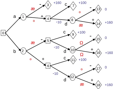
Consider the decision tree in Figure 1. Here the DM must make an initial choice between two actionsaandb, neither of which has an immediate cost. (S)he may need to make a second choice, between two actions c and d, the latter action having an immediate cost of 10 units. The devel-opment of the problem depends at various points on random variables (associated with chance nodes) whose distributions depend on the history of the problem up to that point. Each possible unfolding of the problem has its own associated reward.
[image:8.595.175.409.431.615.2]0 4 5 10 11 14 15 17 18 a b … ‰ … ‰
-+ -+ -+ -+ -+ c d c d c d -10 -10 -10 +160 +100 +100 +100 0 +160 0 +160 0 +160 1 2 3 6 7 8 9 12 13 16 … …Figure 1 Unmodified decision tree
Using Definition 1, we see that
• decision nodes 4, 5 and 6 are in the same proto-stage,
• decision nodes 4 and 6 are in the same stage and in the same position,
• chance nodes 8 and 12 are in the same stage and in the same position,
• utility nodes 3, 14, 16 and 18 are in the same stage and in the same position,
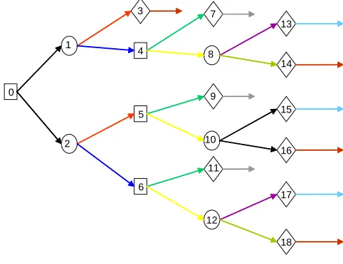
• as are utility nodes 7, 9 & 11 and utility nodes 13, 15 & 17. The resultant coloured decision tree is given in Figure 2
4
12
13
15
16
17
18 0
1
2
3
5
6
7
8
9
10 11
[image:9.595.174.419.253.442.2]14
Figure 2 Coloured decision tree
It is useful here to consider what is meant by v1, v2∈V
D(T) being in the same stage in a little
more detail. If a DM acts in accordance with our assumptions and employs a decision rule which is not a function of whether the process has reachedv1 or v2, then either the difference between the
vertices is inconsequential or the vertices are indistinguishable to her/him. By inconsequential we mean that the consequences (in terms of further costs and rewards) of choosing the same action at each vertex are identical. The difference between two vertices in VD(T) is inconsequential if they
This definition applies to general decision trees. But in an EF tree no pair of vertices
v1, v2∈V
D(T) are ever indistinguishable to the DM as (s)he always knows the outcomes of all
variables encountered prior to making a decision. Hence in an EF tree no pair of decision nodes are ever in the same stage but not the same position, and we can ignore this part of the definition. This isnot true of other types of decision tree.
Clearly any collection of chance nodes in the same position are in the same stage, and any utility nodes in the same stage are necessarily in the same position.
2.3. Conditional independence structure
This coloured decision tree provides us with a formal framework for the DEG representation and propagation rules given in Section 3 and Section 4. It also allows us to read the conditional inde-pendence structure of our problem from the tree, a hitherto almost impossible task.
Dawid (2001) discusses in detail the concepts of conditional independence and irrelevance in the fields of Probability Theory, Statistics, Possibility Theory and Belief Functions. We show how they can be interpreted for coloured decision trees. So consider a set of variables defined on our tree whose outcome spaces can be identified with the set of subpaths connecting two positions or stages, and which may be neither wholly random variables nor wholly decision variables.
Forw∈K(T), letZ(w) be the variable whose outcome spaceZ(w) can be identified with the set of subpaths joining v0 to somev∈w. In general each of these subpaths will consist of a collection
of chance and decision edges.
For u∈L(T), letZ(u) be the variable whose outcome spaceZ(u) can be identified with the set of subpaths joining v0 to somev∈u.
Let Y(w) be the variable whose outcome spaceY(w) can be identified with the set of subpaths emanating from some v∈w and ending in aterminal edge. In general each of these subpaths will consist of a collection of chance and decision edges, plus the one terminal edge.
Also, for v∈VC(T), v∈u∈L(T), let X(u) be the random variable whose values describe the
with the set of directed edgese(v, v′
)∈EC(T) emanating from each v∈u. For each X(u) we let
Π(u)≡ {P(X(u) =e(v, v′
) |v∈u}.
Lastly, let Λ(w) be the event which is the union of all root-to-leaf paths of the tree passing through some v∈w; and Λ(u) be the event which is the union of all root-to-leaf paths passing through somev∈u.
There are two basic collections of conditional independence statements that we can read off an EF tree:
(A) For any w∈K(T), we can write
Y(w)∐Z(w) |Λ(w)
which can be read as:
1. the probability and utility distributions on the edges emanating from any chance node encoun-tered on any subpath y(w)∈Y(w) are not dependent on the vertex v∈w reached;
2. the utility distribution on the edges emanating from any decision node encountered on any subpathy(w), and theconsequences (in terms of further costs and rewards) of any decision made at that decision node are not dependent on the vertex v∈w reached;
3. the utility associated with the edge leaving the utility node on any subpathy(w)is not dependent on the vertex v∈w reached.
So, if we know that a unit has reached some position w, then we do not need to know how our unit reached w (ie. along which v0→v∈w subpath) in order to make predictions about or
decisions concerning the future of the process (ie. along which subpath emanating from v∈w our unit is going to pass).
(B) For any v∈VC(T), v∈u∈L(T), we can write
X(u)∐Z(u) |Λ(u)
of chance nodes, and interpret this statement as follows: The probability and utility distributions on the edges emanating from each v∈u are are not dependent on the vertex v∈u reached.
So, if we know that a unit has reached some stageu(consisting of chance nodes), then we do not need to know how our unit reachedu (ie. along whichv0→v∈usubpath) in order to predict how
the process is going to unfold in the immediate future (ie. by which edge emanating fromv∈uour unit leaves by).
3.
Decision Event Graphs
A DEG is a connected directed acyclic graph which is a function of a decision tree. It differs from the tree in having a single sink node, with every edge lying on some directed path from the root node to the sink node. Additionally, intermediate nodes in the DEG may have multiple incoming edges, whereas in the tree these nodes have only one incoming edge. As with trees, the graphical structure is annotated with the numerical specification of the decision problem.
Definition 2 The Decision Event GraphD(a function of a treeT with positionsK(T) and stages L(T)) is the coloured directed graph with vertex set V(D) and edge set E(D), defined by:
1. V(D) =K(T)∪ {w∞}.
The setV(D)\ {w∞} is partitioned intodecision, chanceandutilitypositions. The subsets of these positions are labelled VD(D), VC(D) and VU(D) respectively.
2. (a) For w, w′
∈V(D)\ {w∞}, there exists a directed edge e(w, w′
) ∈E(D) if f there are vertices v, v′
∈ V(T) such that v ∈ w ∈ K(T), v′ ∈ w′
∈ K(T) and there is an edge e(v, v′
)∈E(T).
(b) For each w∈VU(D) there exists a single directed edge e(w, w∞)∈E(D).
The set E(D) is partitioned into decision, chance and terminal edges, labelled by whether they emanate from decision, chance or utilitypositions. The subsets of these edges are labelled ED(D), EC(D) and EU(D) respectively.
3. If v1∈w1∈K(T), v2∈w2∈K(T), andv1, v2 are members of the same stage u∈L(T), then we say thatw1, w2 are in the same stage u and assign the same colour to these positions. We label
4. (a) If v∈w∈K(T), v′ ∈w′
∈K(T) and there is an edge e(v, v′
)∈E(T), then the edge e(w, w′
)∈E(D) has the same colour as the edgee(v, v′
).
(b) Ifv∈w∈K(T), w∈VU(D), then the edgee(w, w∞)∈E(D) has the same colour as the edge emanating from v∈VU(T).
Example cont.
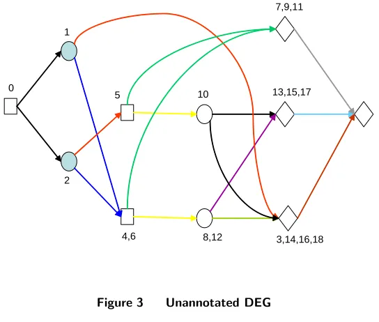
Figure 3 shows the DEG produced from the coloured decision tree in Figure 2 using Definition 2.
10 0
1
2
5
4,6 8,12
7,9,11
13,15,17
[image:13.595.174.446.258.489.2]3,14,16,18
Figure 3 Unannotated DEG
As noted in the introduction, the DEG-representation of a problem may have very different topologies depending on which type of tree it has been derived from. The EF DEG in particular is a good description of how the problem appears to the DM and provides an ideal framework for calculating optimal decisions. Note that in an EF DEG there are no decision nodes which are in the same stage but not the same position.
3.1. Conditional independence structure
conditional independence statements that we can read off an EF DEG.
Consider variables defined on our DEG, analogous to those we have defined on our tree, which have outcome spaces identified with the sets of subpaths connecting two positions or stages.
For w∈V(D)\ {w0, w∞}, let Z(w) be the variable having outcome space Z(w) identified with
the set of subpaths joining w0 to w. For w∈u∈L(D), let Z(u) be the variable having outcome
space Z(u) identified with the union over all w∈u of the sets of subpaths joining w0 to w. Let Y(w) be the variable having outcome space Y(w) identified with the set of subpaths joining w
tow∞. Also, forw∈VC(D), w∈u∈L(D), letX(u) be the random variable whose values describe
the next possible developments in the unfolding process. The state space X(u) of X(u) can be identified with the set of directed edges e(w, w′
)∈EC(D) emanating from each w∈u. For each X(u) we let Π(u)≡ {P(X(u) =e(w, w′
)| w∈u}. Lastly, let Λ(w) be the event which is the union of allw0→w∞paths passing throughw; and Λ(u) be the event which is the union of allw0→w∞
paths passing through somew∈u. Then:
(A) For any w∈V(D)\ {w0, w∞}, we can write
Y(w)∐Z(w) |Λ(w)
which can be read as:
1. the probability and utility distributions on the edges emanating from any chance node encoun-tered on any subpath y(w)∈Y(w) are independent of the subpath taken fromw0 to w;
2. the utility distribution on the edges emanating from any decision node encountered on any subpath y(w), and the consequences of any decision made at that decision node are independent of the subpath taken fromw0 to w;
3. the utility associated with the edge leaving the utility node on any subpathy(w) is independent of the subpath taken fromw0 to w.
If there are no decision nodes on any w→w∞ subpath, then this expression takes its standard meaning for CEGs (Smith et al. (2009)) of
This can be expressed as a conditional probability statement even though if there are decision nodes on anyw0→w subpath, the joint probabilityP(z(w),Λ(w)) is undefined.
So, if we know that a unit has reached some position w, then we do not need to know how our unit reachedwin order to make predictions about or decisions concerning the future of the process.
(B) For any w∈VC(D), w∈u∈L(D), we can write
X(u)∐Z(u) |Λ(u)
For a general DEG we can also define X(u) for decision stages, but as in an EF DEG there are no decision stages which are not positions, we can again restrict our analysis to stages consisting of chance nodes, and interpret this statement as follows: The probability and utility distributions on the edges emanating from each w∈u are independent of both the position w reached, and the
subpath taken from w0 to w.
As we are considering only stages made up of chance nodes, we can write
∀ x(u)∈X(u), z(u)∈Z(u), P(x(u) |z(u),Λ(u)) =P(x(u) |Λ(u))
Again this is a valid expression even if there are decision nodes onw0→w∈u subpaths.
So, if we know that a unit has reached some stage u (consisting of chance nodes) in our EF DEG, then we do not need to know how our unit reachedu in order to predict how the process is going to unfold in the immediate future.
4.
An optimal decision rule algorithm for Decision Event Graphs
is a chance node, then assign a utility value to that position equal to the sum over all child nodes of the product of the probability associated with the edge and the sum of the utility of the child node and the utility associated with the edge (the latter has a default zero if not present). The final possibility is that the position is a decision node, in which case we assign a utility value to that position equal to the maximum value over all child nodes, of the sum of the utility of the child node and the utility value associated with the edge connecting the decision node and the child node. Mark all child edges that do not achieve this maximum value as being sub-optimal.
At the end of the local message passing, the root node will contain the maximum expected utility, and the optimal decision rule will consist of the subset of edges that have not been marked as being sub-optimal. The propagation algorithm is illustrated in the pseudocode below, Table 1. For the pseudocode we use the following notation.VC (abbreviated fromVC(D)),VD andVU represent
respectively the sets of chance, decision and utility nodes. The utility part of a positionw will be denoted by w[u]. Similarly the probability part of an edgee(w, w′) from positionw to positionw′
will be denoted by (w, w′
)[p] and the utility part by (w, w′
)[u]. The set of child nodes of a position w is denoted bych(w).
Table 1 Pseudocode for the backward induction algorithm for finding optimal decision sequence
• Find a topological ordering of the positions. Without loss of generality call thisw0, w1, . . . , wn,
so that w0 is the root node, andwn is the sink node (=w∞). • Initialize the utility valuewn[u] of the sink nodewn to zero. • Iterate: fori=n−1 step minus 1 untili= 0 do:
— Ifwi∈VU then wi[u] = (wi, wn)[u]
— Ifwi∈VC then wi[u] =
P
w′∈
ch(wi)(wi, w ′
)[p]∗(w′[u] + (wi, w ′
)[u])
— Ifwi∈VD then wi[u] = maxw′∈ch(w i)(w
′[
u] + (wi, w′)[u]).
Mark the sub-optimal edges.
and that in the backward induction these are unchanged. Instead the algorithm associates utility values to the receiving nodes.
4.1. A proof of the algorithm
The basic strategy of the proof is to “unwind” the DEG into a decision tree, and show equivalence of local operations on the decision tree to those on the DEG.
Let T denote the underlying EF decision tree of the DEG. Suppose that the i-th position wi
of the DEG has mi distinct paths from the root node to wi; then in T there will bemi vertices {vij:j= 1, . . . , mi}that are coalesced into wi when forming the DEG fromT. Call the number mi
themultiplicity of wi. Note that the root node has multiplicity 1, and that the multiplicity of the
sink node in the DEG counts the number of leaf nodes on the tree. In the tree T each of the mi
decision subtrees rooted at themi vertices in the set {vij:j= 1, . . . , mi} are isomorphic.
Now consider solving the decision problem on the decision tree T. This proceeds by backward induction (Raiffa and Schlaifer 1961) in the same way as in Table 1. Any topological ordering of the vertices of the tree will do, so let us take the following ordering.
v0,1, v1,1, v1,2. . . , v1,m1, v2,1, . . . , v2,m2, . . . , vn,1. . . , vn,mn.
We modify the propagation algorithm to that shown in Table 2 for the decision treeT.
Now because the decision subtrees rooted at themi vertices {vij:j= 1, . . . , mi}are isomorphic,
it follows thatvi,j[u] =vi,k[u] for eachj, k∈ {1, . . . , mi}. By a simple mathematical induction
argu-ment, it also follows thatwi[u] =vi,j[u], wherewi[u] is found from the local propagation algorithm
on the DEG. The induction argument is as follows. Clearly the statement is true fori=n, that is,
wn[u] =vn,j[u]. Assume that it is also true fori=I+ 1, I+ 2, . . . , n. Then in the tree we carry out: • IfwI∈VC then:
Forj= 1 step 1 untilmI do vI,j[u] =
P
v′∈
ch(vI,j)(vI,j, v ′
)[p]∗(v′[u] + (vI,j, v ′
)[u]) • IfwI∈VD then:
Forj= 1 step 1 untilmI do vI,j[u] = maxv′∈ch(v I,j)(v
′
[u] + (vI,j, v ′
Table 2 Backward induction algorithm for the decision tree
• Use the topological orderingv0,1, v1,1, v1,2. . . , v1,m1, v2,1, . . . , v2,m2, . . . , vn,1. . . , vn,mn.
• Initialize the utility values {vn,j[u]|j= 1. . . mn} of all leaf nodes to zero. • Iterate: fori=n−1 step minus 1 untili= 0 do:
— Ifwi∈VU then
∗ For j= 1 step 1 untilmi do vi,j[u] = (vi,j, vn,k)[u] where vn,k is the child leaf node of vi,j
in the tree.
— Ifwi∈VC then
∗ Forj= 1 step 1 untilmi do vi,j[u] =
P
v′∈ch(v
i,j)(vi,j, v ′
)[p]∗(v′[u] + (vi,j, v′)[u])
— Ifwi∈VD then
∗ Forj= 1 step 1 untilmi do vi,j[u] = maxv′∈ch(v i,j)(v
′
[u] + (vi,j, v ′
)[u]). ∗ Mark the sub-optimal edges.
But by the topological ordering, each v′
∈ch(vI,j) is some vk,l vertex for some k≥I+ 1 and l∈ {1, . . . mk}, hence the utility associated with that node is by the induction assumption equal to
that on the wk node in the DEG propagation algorithm. Additionally by construction the edges
emanating fromwI in the DEG are in a one-to-one equivalence with the edges (and have the same
probabilities ifwI is a chance node) emanating from anyvI,j in the tree.
Hence eachj loop in the above algorithm snippet is equivalent to
• IfwI∈VC then:
Forj= 1 step 1 untilmi do vI,j[u] =
P
w′∈ch(w
I)(wI, w ′
)[p]∗(w′[u] + (wi, w′)[u]) • IfwI∈VD then:
Forj= 1 step 1 untilmi do vI,j[u] = maxw′∈ch(w I)(w
′[
u] + (wI, w′)[u]).
But this is identical to the correspondingi=I-th loop in the DEG propagation algorithm, and sowI[u] =vI,j[u] for anyj∈ {1, . . . mI} which proves the induction argument, and thus proves the
5.
An example
We here present a complex problem involving forensic analysis of samples taken from a crime scene, which illustrates the advantages of the DEG in the representation and analysis of asymmetric decision problems. The story is as follows:
The police have a suspect whom they believe broke a window and committed a burglary. They
have the option of asking the forensic service to examine the suspect’s clothing for fragments
of glass from the broken window. If the suspect is indeed the culprit (an event the police give
a 0.8 probability to), then the probabilities that a fragment of glass will be found on his coat or pants are 0.75and 0.4 respectively, these events being independent. If the suspect is not the culprit then the probability of a match is zero. The probability of getting a conviction with a
forensic match is 0.9, and without a match is 0.15.
The costs for analysing the coat and pants are $1000 and $800, or if they are analysed together $1700. The cost of taking the suspect to court is $2600.
The police utility has components of financial cost x and probability of conviction y, and takes the form
U= 25− x
200+ 80y
At various possible points in this procedure the police have to decide from a collection of possible actions — we denote these by
a∨ release the suspect
a∧
go to court
ac test the coat ap test the pants a2 test both together
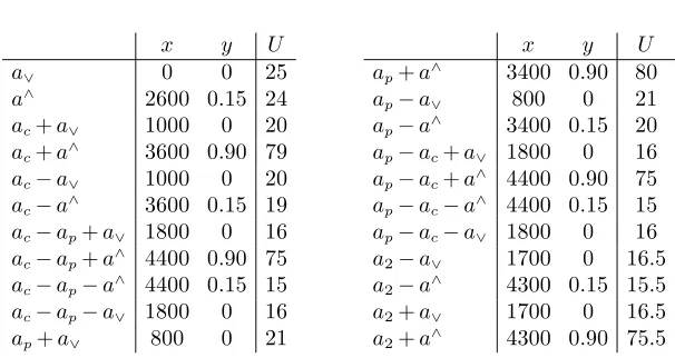
There are 22 different decision / outcome possibilities, each with its own utility. These are listed in Table 3.
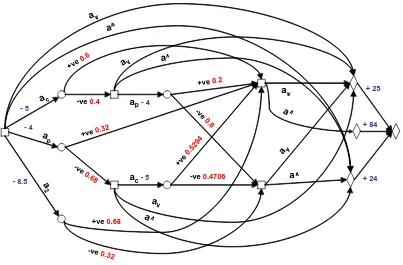
The DEG can be created from the information provided, utilising the symmetries of the problem. There is no need to draw the decision tree first, or to calculate U for each scenario as in Table 3. In the DEG there are 22 root-to-sink paths corresponding to the 22 different decision / outcome possibilities, but there are now only 5 decision nodes and 4 utility nodes. Some preprocessing of probabilities does need to be done, but this is exactly the same as required for the decision tree.
These processed probabilities are added to the edges leaving the chance nodes, and the utilities of the 22 possibilities can be additively decomposed as costs on the edges leaving decision nodes and rewards on the edges leaving utility nodes. The resultant DEG is given in Figure 4. This is an EF DEG, hence there are no decision stages which are not positions. There are also here no chance stages which are not positions. When a DEG obeys both of these conditions we call itsimple
(see Thwaites et al. (2008) for the analogous simple CEG), and we can suppress the colouring of edges and vertices. We have found that a high proportion of problems yield EF DEGs which are simple.
[image:20.595.154.457.565.726.2]The DEG representation has two immediate advantages over the tree — it is much more compact; and the symmetries of the problem (obscured in the tree representation) become apparent. Note also that by decomposing the utilities of the root-to-leaf paths and adding them to appropriate edges, we see exactly what they represent — thecostof analysing the coat is 5 units ($1000÷200) etc. The rewardof taking the suspect to court when there is no positive forensic evidence against him is 24 units, as opposed to the 25 units for releasing him. The rewardfor taking him to court
Table 3 The 22 paths and their utilities
x y U
a∨ 0 0 25
a∧
2600 0.15 24 ac+a∨ 1000 0 20
ac+a ∧
3600 0.90 79 ac−a∨ 1000 0 20
ac−a ∧
3600 0.15 19 ac−ap+a∨ 1800 0 16
ac−ap+a ∧
4400 0.90 75 ac−ap−a
∧
4400 0.15 15 ac−ap−a∨ 1800 0 16
ap+a∨ 800 0 21
x y U
ap+a ∧
3400 0.90 80 ap−a∨ 800 0 21
ap−a ∧
3400 0.15 20 ap−ac+a∨ 1800 0 16
ap−ac+a ∧
4400 0.90 75 ap−ac−a
∧
4400 0.15 15 ap−ac−a∨ 1800 0 16
a2−a∨ 1700 0 16.5
a2−a ∧
4300 0.15 15.5 a2+a∨ 1700 0 16.5
a2+a ∧
ac
a
2
a p
ap- 4
+ 84 + 25
+ 24 - 4
ac- 5
[image:21.595.95.498.86.351.2]+ve 0.6 -ve0.4706 -ve 0.68 -ve0.32 +ve0.68 +ve0.32 - 5 +ve 0.52 94 -ve 0.8 +ve0.2 -ve0.4 - 8.5 a∨∨∨∨ a∧∧∧∧ a∨∨∨∨ a∨∨∨∨ a∨∨∨∨ a∨∨∨∨ a∧∧∧∧ a∧∧∧∧ a∧∧∧∧ a∧∧∧∧
Figure 4 Decision event graph for the forensic example
when there is positive forensic evidence is 84 units.
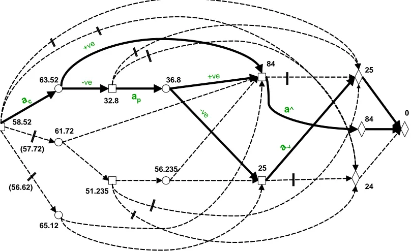
The optimal rule is calculated by working backwards from the sink-node — here there are ten chance and decision nodes compared to the sixteen in the underlying tree. In Figure 5 suboptimal paths are marked and the optimal rule has been indicated in bold. The optimal rule, which gains a rewardof 58.52 units, is to test the coat — if a positive result is obtained take the suspect to court, if not test the pants — if a positive result is obtained take the suspect to court, otherwise release him. Finding this rule and calculating the expected utility are clearly quicker than when performing the same calculations directly on the framework of the tree.
63.52
65.12 61.72
56.235
51.235
36.8
84
25
24 32.8
(57.72) 58.52
(56.62)
25
84 0
a∧∧∧∧
a∨∨∨∨ ac
+ve
-ve
ap
+ve
[image:22.595.99.503.269.516.2]-ve
Figure 5 Decision event graph for the forensic example, showing optimal paths
The flexibility of the DEG is a direct consequence of the fact that the conditional independence structure of the problem is stored in the topology of the graph. It gives the DEG additional advantages over the tree. Thus suppose we need to examine the impact of changes in the utility function, and consider the cost of testing the coat rising to 7 units ($1400). Using the tree we would have to revise all branches utilising the edges leaving the root-node labelledac andap, and revise
are those connected with the nodes associated with testing the pants, testing the pants and getting a−veresult, and the root-node. There is a similar gain in efficiency over the tree if we change, say, the probability of getting a positive result from testing the pants. This type of flexibility, exhibited by IDs for a much more restrictive class of decision problems, is a characteristic feature of DEGs.
6.
Simplifying results
There are a number of highly useful results which allow us to increase the efficiency of our algorithm for finding optimal decision rules, and to simplify the specification of a decision process so that it expresses only attributes that might have a bearing on the choice of an optimal action. These allow the preprocessing of an elicited DEG, transforming it to one with a simpler topology which embodies all the information from the structure of the problem needed to discover an optimal policy. This is often a valuable step to make since the transformation allows us to deduce that certain quantitative information which we might elicit will have no impact on the consequences of our decisions. So we learn from the DEG which information need not be collected. This type of preprocessing is commonly performed when a decision problem is represented as an ID. However the analogous transformations of DEGs are more powerful and apply to a much wider range of decision problems. We illustrate some of these transformations below.
6.1. Path reduction
If every path from some positionw1∈V(D) passes through some subsequent positionw2, and every
edge of every subpath µ(w1, w2) has zero associated utility, then the set of subpaths{µ(w1, w2)}
can be replaced by a single edge e(w1, w2) with zero associated utility. This highly useful result is
expressed in the following lemma, for which we introduce some extra notation.
Let S(w1, w2) be the set of subpaths connectingw1 andw2; Λ(wa, wb) be the event which is the
union of allw0→w∞ paths passing through the positionswa andwb; Λ(wa, e) be the event which
is the union of all w0→w∞ paths passing through the position wa and the edge e; w∈µ be a
position lying on the subpath µ; ande∈µ be an edge lying on the subpathµ.
subsequent position w2∈V(D) (6=w∞), and every subpath µ(w1, w2) has zero associated utility, then there is a DEG Dˆ where
V( ˆD) =V(D)\ {w∈µ |w6=w1, w2, Λ(w1, w)≡Λ(w), µ∈S(w1, w2)}
E( ˆD) =E(D)\ {e∈µ |Λ(w1, e)≡Λ(e), µ∈S(w1, w2)} ∪ˆe(w1, w2)
where eˆ(w1, w2) has zero associated utility, and such that an optimal decision rule for Dˆ is an optimal decision rule for D.
This Lemma (for proof see the Appendix) is particularly useful when our DEG does not have utilities decomposed onto edges, but also has applications when there are utilities attached to edges. It has an analogue inbarren node deletion (Shachter (1986)). If a problem can be represented by both a DEG and an ID, then the DEG can always be constructed so that the edges corresponding to the outcomes of a collection of barren nodes on the ID form collections of subpaths of the
w0→w∞paths of the DEG. Moreover these subpaths correspond to vectors of outcomes of vertices
in the ID which have no directed paths from them to the utility node, so these outcomes have no effect on the value of the utility function and consequently the utilities attached to each of these subpaths is zero.
There is a similar result when every path from a position w1 ∈V(D) (6=w0) passes through
some subsequent positionw2∈V(D) (=6 w∞), but the subpathsµ(w1, w2) have different associated
utilities. The graph rooted inw1and havingw2 as a sink is itself a DEG. Optimal decision analysis
can be performed separately on this sub-DEG and nested in the analysis for the full DEG. These ideas can be used to reduce the length and complexity of collections of subpaths between non-adjacent nodes in isolation from other parts of the DEG. Once one collection has been tackled, other collections can be investigated, and this piecemeal approach suits asymmetric problems, as some parts of the graph may simplify more readily than others.
6.2. Parsimony
w∈VD(D)).
In an Extensive form ID we can uniquely specify the variables preceding and succeeding any decision variable D. Labelling these by Z(D), Y(D) respectively, a parsimonious DM using this EF ID is one who, if when arriving at a decision variable Dand finding that
U ∐ R(D) |(D, Q(D)) (1)
for some partition Z(D) =R(D)∪Q(D), ignores R(D) (Smith (1996)).R(D) are the redundant
parents andQ(D) are thesufficient parents ofD.
It is reasonable to specify that the EF ID has had any barren nodes removed, and for such a graph, statement (1) is equivalent to
Y(D) ∐R(D)|(D, Q(D)) (2)
But if a DM ignores R(D) then it is irrelevant for D (if Q(D) is known). This can therefore be expressed as
D ∐R(D) |Q(D) (3)
But in any irrelevance system, · ∐ · | · must satisfy the property that X ∐ (Y, Z) | W ⇔ {X∐Y |(Z, W), X∐Z |W}(Smith (1989b) Dawid (2001)), so expressions (2) and (3) both hold if and only if
(D, Y(D))∐R(D)| Q(D) ≡(D, Y(D))∐Z(D)|Q(D) (4)
Consider now an EF DEG of our problem, where the DM has to make a decision associated withD
on each w0→w∞ path. Then there exists a set W ⊂VD(D) of decision positions associated with
the variable D. An outcome of Q(D) (the sufficient parents of D) then corresponds to Λ(w) for some w∈W; Z(D) corresponds to Z(w) when conditioned on this Λ(w); and an outcome of D
together with an outcome ofY(D) corresponds to a pathY(w) when conditioned on Λ(w). So the analogous expression to (4) for EF DEGs is
A DM using an EF DEG is parsimonious by disregarding information in Z(w) other than Λ(w). This allows the DM to simplify the topology of the DEG in an analogous manner to that in which a parsimonious DM can simplify the topology of an ID (Smith 1996), which in turn allows the DM to deduce information about the problem which it is unnecessary to elicit.
7.
Discussion
In this paper we have introduced a new graphical representation of multistage decision problems, called theDecision Event Graph(DEG), which is suited to asymmetric decision problems. We have shown how the structure may be used to find optimal decision policies by a simple local backward induction algorithm.
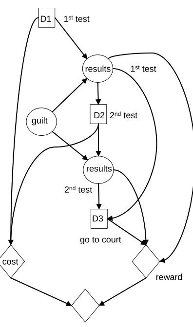
The focus of this paper has been on the relationship between DEGs and decision trees. The relationship between DEGs and IDs is too substantial a topic to do any more than touch upon here, but there are a couple of points which can be made quickly – ID-representations of asymmetric problems are at best a compromise, and storing the numerical specification of such problems is inefficient when compared with a DEG-representation. These can both be seen if we consider the example from Section 5. In order to create an ID for this problem we would have to impose a product space structure and accept that the inherent asymmetries would produce a considerable number of zeroes in our tables. If we do this then the ID in Figure 6 is probably the simplest of a number which could be drawn. Using this graph numerical specification would require 74 cells, whereas with the DEG we need at most 24 cells. Note also that although the ID may appear simpler than the DEG, it does not depict sample information which is explicit in the DEG. With both the DEG and the ID there are tweaks which could be made to the graph and / or the storage tables which reduce the storage costs, albeit with some loss to the integrity of the representation. There is a similar increased efficiency for the DEG algorithm over the analogous ID algorithms.
We return to the relationship between DEGs and IDs in a forthcoming paper in which we also develop the ideas from Section 6. Software for finding optimal decision rules on EF DEGs is currently being coded and will be freely available shortly.
D1 1sttest
results 1sttest
guilt
results
2ndtest
D3
go to court D2 2ndtest
[image:27.595.210.408.94.430.2]reward cost
Figure 6 Influence diagram for the forensic example
We believe that the power and acceptance of the influence diagram comes from a graphical
method that is interpretable by both professions and lay-people, and that can contain in-depth
technical information to completely characterize any decision. The diagram provides a common
language for representing both uncertain relationships and decision problems in a wide variety
of applications.
Because of their greater generality, we hope that a similar acceptance will develop in the future for decision event graphs.
Appendix. Proof of Lemma 1
Consider a set{w} ⊂V( ˆD) which partitions thew0→w∞paths of ˆD, and which contains the positionw1.
(1) Λ(w, w2) =φ
(2) w≺w2but Λ(w1, w) =φ
(3) w=w1
For cases (1), (2) there exist sub-DEGs inD, ˆDrooted inw, whose topology, edge labels, edge probabilities and edge utilities are identical in each graph. So in cases (1), (2), w[u]Dˆ=w[u]D.
For case (3), by construction, w1[u]Dˆ=w1[u]D=w2[u]D.
The subgraphs ofD,Dˆ rooted in w0 and with the elements of{w} as leaves have identical topology, edge
labels, edge probabilities and edge utilities. Hence by backward induction, w0[u]Dˆ=w0[u]D.
The optimal decision rule is found by moving forward (downstream) from w0. If in Dthis does not take
us tow1, then it will not in ˆD, and the optimal decision rule is unchanged.
If inDthe rule takes us tow1, then it also takes us tow2 with probability 1, and any decisions made at
w1or betweenw1andw2 are irrelevant as allµ(w1, w2) subpaths have zero associated utility. In ˆDthe rule
takes us tow1, w2, and downstream ofw2 is unchanged fromD.
Acknowledgments
This research has been partly funded by the UK Engineering and Physical Sciences Research Council as part of the projectChain Event Graphs: Semantics and Inference(grant no. EP/F036752/1).
References
C. Bielza and P. P. Shenoy. A comparison of graphical techniques for asymmetric decision problems. Man-agement Science, 45(11):1552–1569, 1999.
C. Boutilier. The influence of influence diagrams on artificial intelligence. Decision Analysis, 2(4):229–231, 2005.
H. J. Call and W. A. Miller. A comparison of approaches and implementations for automating decision analysis. Reliability Engineering and System Safety, 30:115–162, 1990.
R. G. Cowell. Decision networks: a new formulation for multistage decision problems.Research Report 132, Department of Statistical Science, University College London, London, United Kingdon, 1994.
R. G. Cowell, A. P. Dawid, S. L. Lauritzen, and D. J. Spiegelhalter. Probabilistic Networks and Expert Systems. Springer, New York, 1999.
A. P. Dawid. Separoids: A mathematical framework for conditional independence and irrelevance. Annals of Mathematics and Artificial Intelligence, 32:335–372, 2001.
R. A. Howard and J. E. Matheson. Influence diagrams. In R. A. Howard and J. E. Matheson, editors, Readings in the Principles and Applications of Decision Analysis. Strategic Decisions Group, Menlo Park, California, 1984.
R. A. Howard and J. E. Matheson. Influence diagram retrospective. Decision Analysis, 2(3):144–147, 2005.
F. Jensen, F. V. Jensen, and S. L. Dittmer. From influence diagrams to junction trees. In R. L. de Mantaras and D. Poole, editors, Proceedings of the 10th Conference on Uncertainty in Artificial Intelligence, pages 367–373, San Francisco, California, 1994. Morgan Kaufmann.
F. V. Jensen and T. D. Nielsen. Bayesian networks and decision graphs. Springer, 2007. 2nd edition.
R. L. Keeney and H. Raiffa. Decisions with multiple objectives: Preferences and Value trade-offs. Wiley, New York, 1976.
D. V. Lindley. Making Decisions. John Wiley and Sons, Chichester, United Kingdom, 1985.
S. M. Olmsted. On Representing and Solving Decision Problems. Ph.D. Thesis, Department of Engineering– Economic Systems, Stanford University, Stanford, California, 1983.
J. Pearl. Influence diagrams—historical and personal perspectives. Decision Analysis, 2(4):232–234, 2005.
H. Raiffa. Decision Analysis. Addison–Wesley, Reading, Massachusetts, 1968.
H. Raiffa and R. Schlaifer.Applied Statistical Decision Theory. MIT Press, Cambridge, Massachusetts, 1961.
R. D. Shachter. Evaluating influence diagrams. Operations Research, 34:871–882, 1986.
P. P. Shenoy. Representing and solving asymmetric decision problems using valuation networks. In D. Fisher and H.-J. Lenz, editors, Learning from Data: Artificial Intelligence and Statistics V, pages 99–108. Springer–Verlag, New York, 1996.
J. Q. Smith. Bayesian Decision Analysis: Principles and Practice. CUP, 2010. (to appear).
J. Q. Smith. Influence diagrams for Bayesian decision analysis. European Journal of Operational Research, 40:363–376, 1989a.
J. Q. Smith. Influence diagrams for statistical modelling. Annals of Statistics, 7:654–672, 1989b.
J. Q. Smith. Plausible Bayesian Games. In J. M. Bernardo, J. O. Berger, A. P. Dawid, and A. F. M. Smith, editors,Bayesian Statistics 5, pages 387–402. Oxford, 1996.
J. Q. Smith and P. E. Anderson. Conditional independence and chain event graphs. Artificial Intelligence, 172:42–68, 2008.
J. Q. Smith and P. A. Thwaites. Decision trees. InEncyclopedia of Quantitative Risk Analysis and assessment, volume 2, pages 462–470. Wiley, 2008a.
J. Q. Smith and P. A. Thwaites. Influence diagrams. In Encyclopedia of Quantitative Risk Analysis and assessment, volume 2, pages 897–909. Wiley, 2008b.
J. Q. Smith, E. Riccomagno, and P. Thwaites. Causal analysis with chain event graphs. Submitted to Artificial Intelligence, 2009.